Formation of clusters in the $2D$ $t-J$ model: The mechanism for phase separation.

Abstract

The emergence of phase separation is investigated in the framework of a $2D$ $t-J$ model by means of a variational product ansatz, which covers the infinite lattice by two types of $L\times L$ clusters. Clusters of the first type are completely occupied with electrons, i.e. they carry maximal charge $Q_{e}=L^{2}$ and total spin 0, and thereby form the antiferromagnetic background. Holes occur in the second type of clusters – called “hole clusters”. They carry a charge $Q_{h}<L^{2}$. The charge $Q_{h}$ and the number $N(Q_{h})$ of hole clusters is fixed by minimizing the total energy at given hole density and spin exchange coupling $\alpha=J/t$. For $\alpha$ not too small ($\alpha>0.5$) it turns out that hole clusters are occupied with an even number $Q_{h}<L^{2}$ of electrons and carry a total spin 0. For increasing $\alpha$ the charge $Q_{h}(\alpha)$ of the hole clusters decreases. Some points on the boundary curve can be extracted from $Q_{h}(\alpha)$.

1 Introduction

Holes play a fundamental role in our understanding of high $T_{c}$ superconductivity.[1] The parent materials like $La_{2}CuO_{4}$ are insulators with antiferromagnetic order and doping with holes (missing electrons) opens the superconducting phase. [2]

Experimental evidence has been found in $La_{2}CuO_{4+\delta}$ for phase separation.[3, 4, 5, 6] This means that the holes in the $CuO_{2}$ planes are not distributed uniformly but concentrate in “hole rich” domaines. The compound phase separates for $0.01\leq\delta\leq 0.06$ below $T_{ps}\sim 300K$ into the nearly stoichiometric antiferromagnetic $La_{2}CuO_{4+\delta_{1}}$ with $\delta_{1}<0.02$ and Néel temperature ($T_{N}\simeq 250K$), and a metallic superconducting oxygen-rich phase $La_{2}CuO_{4+\delta_{2}}$ with $\delta_{2}\approx 0.02$ and $T_{c}\simeq 34K$. The other evidence is related to the $Sr$ doped compound $La_{2-x}Sr_{x}CuO_{4+\gamma}$. This compound phase separates for $x\leq 0.03$ into the superconducting $La_{2-x}Sr_{x}CuO_{4+\gamma_{1}}$ ($\gamma_{1}\approx 0.08$) and the nonsuperconducting $La_{2-x}Sr_{x}CuO_{4+\gamma_{2}}$ ($\gamma_{2}\approx 0.00$) phases. [7]

Intensive studies have been performed to understand this phenomenon in models for strongly correlated electrons like the Hubbard – and $t-J$ model. In the $2D$ $t-J$ model various attempts have been made to exploit the phase diagram in the plane spanned by the charge density $\rho=Q_{\mbox{tot}}/N$ and the spin coupling $\alpha=J/t$ ($N$, $Q_{\mbox{tot}}$ denote the total numbers of sites and electrons, respectively).

Phase separation occurs, if both the charge density $\rho$ and the spin coupling $\alpha$, are large enough

$$1\geq\rho\geq\rho_{1} \alpha>\alpha_{p}(\rho_{1})\,.$$ , (1)

In this regime, the ground state can be represented by a product ansatz

$$\psi(\rho,N)=\psi_{e}\Big{(}N_{e}(\rho)\Big{)}\psi_{h}\Big{(}N_{h}(\rho,\rho_{1})\Big{)}$$ (2)

of two clusters with site numbers $N_{e}(\rho)$ and $N_{h}(\rho,\rho_{1})$, which cover the whole lattice:

$$N_{e}(\rho)+N_{h}(\rho,\rho_{1}) = N\,.$$ (3)

The $N_{e}(\rho)$ sites in the “electron” cluster are all occupied with electrons. The corresponding ground state $\psi_{e}(N_{e}(\rho))$ is just the ground state of the $2D$ Heisenberg model with $N_{e}(\rho)$ sites. Holes occur in the “hole” cluster with $N_{h}(\rho,\rho_{1})$ sites. The corresponding ground state $\psi_{h}(N_{h}(\rho,\rho_{1}))$ is given by the $t-J$ model with $N_{h}(\rho,\rho_{1})$ sites and $Q_{h}=N_{h}(\rho,\rho_{1})\rho_{1}$ electrons. The numbers $N_{e}(\rho)$ and $N_{h}(\rho,\rho_{1})$ for the cluster sites are fixed by the total number of sites (3) and the total number of electrons

$$N_{e}(\rho)+\rho_{1}N_{h}(\rho,\rho_{1}) = Q_{\mbox{tot}}\,.$$ (4)

From (2)-(4) one derives that the ground state energy per site $\varepsilon(\rho,\alpha)$:

$$\varepsilon(\rho,\alpha) = \frac{1}{1-\rho_{1}}\left[\varepsilon(\rho_{1},\alpha)(1-\rho)+\varepsilon(1,\alpha)(\rho-\rho_{1})\right]$$ (5)

is linear in $\rho$. This holds for (1), i.e. in the region with phase separation.

The focus is the boundary curve $\alpha_{p}(\rho_{1})$ for phase separation. Two controversary points of view can be found in the literature: Emery et al.[8] suggested that in the $2D$ $t-J$ model the phase separation curve $\alpha_{p}(\rho_{1})$ starts at $\alpha_{p}(\rho_{1}=1)=0$, which means that phase separation exists already for low doping $(1-\rho_{1})\simeq 0$ and small values of $\alpha$, as observed experimentally.[3] Their point of view is supported by Hellberg and Manousakis [9, 10, 11, 12].

On the other hand Putikka et al.[13, 14] concluded from a high temperature expansion, that phase separation at low doping only emerges for larger $\alpha$ values $\alpha>\alpha_{p}(\rho_{1}=1)\simeq 1.2$, which would exclude the $\alpha$ regime realized in the experiments. This point of view is supported by DMRG calculationss on ladders (Rommer, White, Scalapino[15]), variational wave functions of the Luttinger-Jastrow-Gutzwiller type (Valenti, Gros[16]), Lanczos calculations (Dagotto[17, 18]).

Finally, Green’s function Monte-Carlo simulations performed by Calandra et al. (CBS)[19] led to a value $\alpha_{p}(\rho_{1}=1)\simeq 0.5$.

In this paper, we would like to study the mechanism of phase separation by means of a product ansatz with $L\times L$ clusters of charge $Q$ which cover the infinite lattice. Our method is in the spirit of the coupled cluster method (CCM) designed almost 50 years ago [20] as an approximation scheme for quantum many body problems. In order to handle the interaction between clusters, perturbative [21] and variational [22] methods have been implemented. In our study of the phase diagram in the ($\rho=Q/N,\alpha=J/t$) plane, we proceed as follows: We start from the ground states $\psi^{(L)}(\rho_{1},\alpha)$ with energies $E^{(L)}(Q_{1},\alpha)$ on $L\times L$ clusters with charge $Q_{1}=\rho_{1}L^{2}$. These ground states can be computed analytically for plaquette clusters ($L=2$). In Section 2 we will discuss the product ansatz with plaquette clusters, which minimizes the total energy at fixed charge density $\rho=Q/N$. Phase separation can be observed on the small plaquette cluster on a “microscopic scale”.

In Section 3 we extend our considerations to clusters of size $L\times L$. Results for the phase diagram obtained from a numerical calculation of ground state energies on a $4\times 4$ cluster are shown. We finally summerize and present the discussion in Section 4.

2 Plaquette cluster in the $t-J$ model: Phase separation “in statu nascendi”

We start from the $t-J$ model in two dimensions which is built up as a lattice of $L\times L$ clusters (cf. Fig. 1 for the example of $L=2$):

$$H = t\sum_{i}h_{p_{i}}(\alpha=J/t)+t^{\prime\prime}\sum_{\langle i,j\rangle}h_{p_{i},p_{j}}(\alpha)$$ (6)

with $h_{p_{i}}$ and $h_{p_{i},p_{j}}$ containing all nearest neighbour bonds $\langle k,l\rangle$ in a cluster $p_{i}$ or between neighbouring clusters ($p_{i}$, $p_{j}$), respectively. In general, each nearest neighbour bond $\langle k,l\rangle$ of the lattice either belongs to a cluster (parameters $t,J=\alpha t$) or connects neighbouring clusters ($t^{\prime\prime},J^{\prime\prime}=\alpha t^{\prime\prime}$) and contributes with $th^{(k,l)}(\alpha)$ or $t^{\prime\prime}h^{(k,l)}(\alpha)$ to the respective intra- or inter-cluster part of the Hamiltonian (6):

$$h^{(k,l)}(\alpha)={\cal P}\Big{[}-\sum_{\sigma}\left(c_{k,\sigma}^{+}c_{l,\sigma}+\mbox{h.c.}\right)+\alpha\Big{(}{\bf S}_{k}\cdot{\bf S}_{l}-\frac{1}{4}n_{k}n_{l}\Big{)}\Big{]}{\cal P}$$ (7)

where

$$n_{l} = \sum_{\sigma}n_{l,\sigma}=\sum_{\sigma}c_{l,\sigma}^{+}c_{l,\sigma}$$ (8)

and ${\cal P}$ projects onto the subspace where the occupation numbers $n_{l}$ are restricted to zero or one. The electron spin operator is represented by ${\bf S}_{k}$ at the k-th site.

The interaction between $L=2$ clusters is mediated by the two dashed links for each spatial dimension. It is treated in the following by a perturbation expansion in the hopping parameter $t^{\prime\prime}$, which allows the hopping of electrons between neighbouring plaquettes.

Figure 1: $2D$ lattice structure with underlying $2\times 2$ plaquette structure.

To zeroth order in $t^{\prime\prime}$, the eigenstates of the $2D$ $t-J$ model decay into a product

$$\prod_{p}|Q_{p}\rangle$$ (9)

of plaquette eigenstates $|Q_{p}\rangle$ with charge $Q_{p}$. The ground state is characterized by a minimum of the energy:

$$E_{0}=\sum_{p}E^{(p)}(Q_{p}) = \sum_{Q=0}^{4}E^{(p)}(Q)N(Q)$$ (10)

where $N(Q)$ is the number of plaquettes with charge $Q=0,1,2,3,4$. $E^{(p)}(Q)$ is the ground state energy of a plaquette with charge $Q$.

The numbers $N(Q)$ are constrained by the total number of plaquettes ($N/4$) and the total charge ($Q_{\mbox{tot}}$):

$$\sum_{Q=0}^{4}N(Q)=N^{(p)}=\frac{N}{4} \quad,\quad \sum_{Q=0}^{4}QN(Q)=Q_{\mbox{tot}}$$ (11)

The plaquette ground state energies $E^{(p)}(Q)$ have been computed in Appendix A of Ref. [23]. The there obtained formulas simplify for the symmetric case we are considering here.

In the charge sectors $Q=0,1,2,4$ there is no level crossing and the plaquette ground state energy for all $\alpha>0$ reads

$$E^{(p)}(0) = 0\hskip 113.81102ptS=0$$ (12)

$$E^{(p)}(1) = -2t\hskip 96.73918ptS=1/2$$ (13)

$$E^{(p)}(2) = -\frac{t}{2}\Big{(}\alpha+\sqrt{\alpha^{2}+32}\Big{)}\hskip 15.6491ptS=0$$ (14)

$$E^{(p)}(4) = -3t\alpha\hskip 89.626ptS=0$$ (15)

Note that the total spin ${\bf S}^{(p)}$ of the plaquette electrons commutes with the plaquette Hamiltonian and the eigenvalues of ${{\bf S}^{(p)}}^{2}=S(S+1)$ can be used to characterize the plaquette ground state. This plays an important role in the sectors with $Q=3$ where the ground state changes with $\alpha$:

$$E_{I}^{(p)}(3,\alpha) = -2t,\hskip 88.20354ptS=3/2\hskip 8.53581pt\mbox{for}\hskip 8.53581pt0\leq\alpha\leq\alpha_{m}$$

$$E_{II}^{(p)}(3,\alpha) = -t\Big{(}\alpha+\sqrt{\frac{\alpha^{2}}{4}+3}\Big{)},\hskip 14.22636ptS=1/2\hskip 14.22636pt\mbox{for}\hskip 14.22636pt\alpha_{m}\leq\alpha<2$$

$$E_{III}^{(p)}(3,\alpha) = -t\Big{(}\frac{3\alpha}{2}+1\Big{)},\hskip 48.36967ptS=1/2\hskip 14.22636pt\mbox{for}\hskip 14.22636pt\alpha>2.$$ (16)

with $\alpha_{m}=\frac{2}{3}(4-\sqrt{13})=0.262..$.

Note, that the Nagaoka ferromagnetic state[24] – with maximal spin $S=Q/2$ – is already visible on a 4-site plaquette with one hole, i.e. $Q=3$, if $\alpha$ is small enough $\alpha<\alpha_{m}=0.262$. Eigenstates with maximal plaquette spin $S=Q/2$ exist in all charge channels; the corresponding energy eigenvalues $E(Q,S=Q/2)$ do not depend on the spin exchange coupling $\alpha$. However, these eigenstates are not ground states except for the one hole case.

Let us next look for the minimum of the total energy (10), which depends on the relative magnitude of the plaquette energies.

• In the regime, where the inequality

  $$E^{(p)}(4)+E^{(p)}(2) < 2E^{(p)}(3)$$ (17)

  holds, two plaquettes with charge $Q=3$ are substituted by two plaquettes with charges $Q=2$ and $Q=4$, respectively. Insertion of the ground state energies [(14), (15), (16)] yields the validity of (17) for

  $$\alpha > \alpha(3)=\frac{2}{\sqrt{21}}\simeq 0.436\,.$$ (18)

• The inequalitiy

  $$E^{(p)}(0)+E^{(p)}(4) < 2E^{(p)}(2)$$ (19)

  holds for

  $$\alpha \geq \alpha(2)=4\sqrt{2/3}\simeq 3.266$$ (20)

  and allows the substitution of the charge $Q=2$ plaquettes.

• The inequality

  $$E^{(p)}(0)+E^{(p)}(2) < 2E^{(p)}(1)$$ (21)

  holds for

  $$\alpha > 2$$ (22)

  and allows to substitute $Q=1$ plaquettes.

Fig. 2(A) shows a schematic view of the phase diagram in the $\rho-\alpha$ plane with the pairs of plaquette charges, which fix the ground state energy per site according to eqs. (10)-(11).

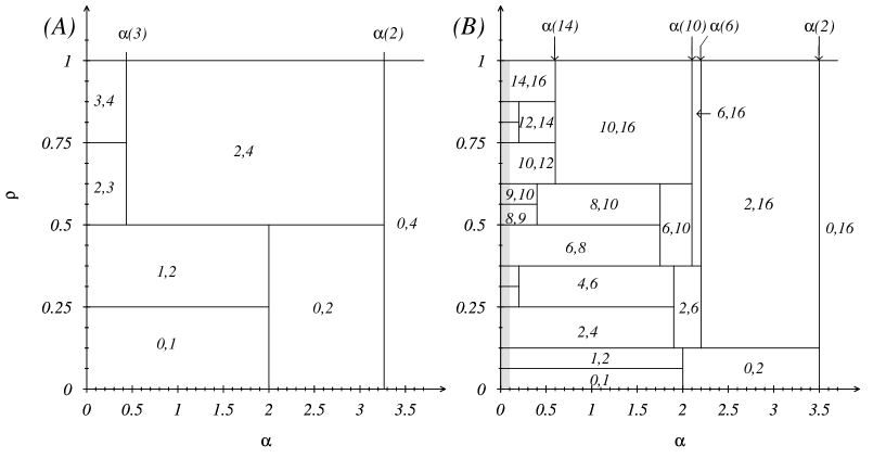
Figure 2: Schematic phase diagram obtained from $2\times 2$ plaquettes (A) and $4\times 4$ plaquettes (B). The charges $Q_{1},Q_{2}$ that constitute the respective ground states in the $\rho-\alpha$-planes and the boundaries $\alpha(2j)$ are given in the text.

In each of the domains with plaquette pairs $Q_{1},Q_{2}$

$$Q_{1}<Q_{2} \frac{Q_{1}}{N_{c}}<\rho<\frac{Q_{2}}{N_{c}}$$ (23)

where the plaquette sites $N_{c}=4$, the ground state energy per site:

$$\varepsilon(\rho,\alpha)=\frac{1}{Q_{2}-Q_{1}}\Big{\{}E^{(p)}(Q_{1})\Big{(}\frac{Q_{2}}{N_{c}}-\rho\Big{)}+E^{(p)}(Q_{2})\Big{(}\rho-\frac{Q_{1}}{N_{c}}\Big{)}\Big{\}}$$ (24)

is linear in $\rho$ and the chemical potential $\mu(\rho,\alpha)=d\varepsilon/d\rho$ is constant with respect to $\rho$. Note that two domains ($Q_{1},Q_{2}$) and ($Q_{2},Q_{3}$) with a common plaquette charge $Q_{2}$ have also a common horizontal boundary at charge density $\rho_{2}=Q_{2}/4$. At this boundary the chemical potential $\mu(\rho,\alpha)$ as function of $\rho$ is discontinuous with a jump

$$\Delta(Q_{2},\alpha) = \mu(\rho+0,\alpha)-\mu(\rho-0,\alpha)$$ (25)

$$= \frac{E^{(p)}(Q_{3})}{Q_{3}-Q_{2}}+\frac{E^{(p)}(Q_{1})}{Q_{2}-Q_{1}}-\frac{Q_{3}-Q_{1}}{(Q_{3}-Q_{2})(Q_{2}-Q_{1})}E^{(p)}(Q_{2})$$

which vanishes for a specific value of $\alpha=\alpha(Q_{2})$. They define the vertical lines in the phase diagram given by (18), (20) and (22). This type of phase diagram has been introduced first by Kagan et al. [25] for the three leg ladder in the rung cluster approximation. Note, that the constraints for ($N^{(p)}$, $Q_{\mbox{tot}}$)(11) are taken into account explicitely on both sides of the inequalities (17), (19), (21). This procedure can be considered as an alternative to the usual grand canonical one, where the charge conservation constraint (11) is eliminated by a reservoir with a fixed chemical potential.

3 Product ansatz for the ground state with large clusters

The considerations which led to the phase diagram in Fig. 2(A) based on plaquette clusters can easily be extended to larger $L\times L=N_{c}$ clusters with $N_{c}$ sites and charges $Q=N_{c},\ldots,0$. We start with the ground state energies $E(Q,N_{c},\alpha)$ and their dependence on $\alpha$. The generalization of (24) to a cluster with $N_{c}$ sites and charges $Q_{1}<Q_{2}$ is straightforward by replacing $E^{(p)}(Q_{1})\rightarrow E(Q_{1},\alpha,N_{c})$. Again the ground state energy per site is linear in $\rho$ and the chemical potential is constant:

$$\mu(\rho,\alpha) = \frac{1}{Q_{2}-Q_{1}}\Big{\{}E(Q_{2},\alpha,N_{c})-E(Q_{1},\alpha,N_{c})\Big{\}}\,.$$ (26)

Two domains ($Q_{1},Q_{2}$) ($Q_{2},Q_{3}$) with a common cluster charge $Q_{2}$ have a common boundary in the phase diagram at $\rho_{2}=Q_{2}/N_{c}$. At this boundary the chemical potential is discontinuous with a jump

$$\Delta(Q_{2},\alpha) = \mu(\rho_{2}+0,\alpha)-\mu(\rho_{2}-0,\alpha)$$ (27)

$$= \frac{E(Q_{3})-E(Q_{2})}{Q_{3}-Q_{2}}-\frac{E(Q_{2})-E(Q_{1})}{Q_{2}-Q_{1}}$$

which vanishes for a specific value of $\alpha=\alpha(Q_{2})$. The inequality

$$\Delta(Q_{2},\alpha) < 0\quad\mbox{for\quad}\alpha>\alpha(Q_{2})$$ (28)

means that the clusters with charge $Q_{2}$ and ground state energy $E(Q_{2},\alpha,N_{c})$ can be substituted by clusters with charges $Q_{3}$ and $Q_{1}$ and energies $E(Q_{3},\alpha,N_{c})$, $E(Q_{1},\alpha,N_{c})$. Here the two domains ($Q_{1},Q_{2}$) ($Q_{2},Q_{3}$) merge for $\alpha>\alpha(Q_{2})$ and the ground state is given by a cluster product ansatz with charges ($Q_{1},Q_{3}$).

Let us first consider the case [case ($A$)]

$$Q_{1}=Q_{2}-1,\,\,Q_{3}=Q_{2}+1,\,\, Q_{2}\quad\mbox{odd},\,\,\alpha<\alpha(Q_{2})\,.$$ (29)

Here the ground state is built up from clusters with charges:

$$(Q_{2}-1,\,Q_{2}) \frac{Q_{2}-1}{N_{c}}\leq\rho\leq\frac{Q_{2}}{N_{c}}$$ for (30)

$$(Q_{2},\,Q_{2}+1) \frac{Q_{2}}{N_{c}}\leq\rho\leq\frac{Q_{2}+1}{N_{c}}\,.$$ for (31)

The vanishing of the jump (27) in the chemical potential

$$\Delta(Q_{2},\alpha(Q_{2})) = E(Q_{2}+1)+E(Q_{2}-1)-2E(Q_{2})=0$$ (32)

defines the boundary $\alpha=\alpha(Q_{2})$, where the two domains (30) and (31) merge together:

$$(Q_{2}-1,\,\,Q_{2}+1)\quad\mbox{for\quad}\frac{Q_{2}-1}{N_{c}}\leq\rho\leq\frac{Q_{2}+1}{N_{c}}\hskip 14.22636pt\mbox{and}\,\,\alpha>\alpha(Q_{2}).$$ (33)

The numerical evaluation of (32) from the ground state energies on a $4\times 4=16$ cluster – with periodic boundary conditions – yields the couplings $\alpha(Q_{2})$ listed in Table 1 (col. 1,2):

Table 1: Boundary couplings $\alpha(Q_{2})$ [from left to right cases ($A$), ($B$), ($C$)] where the jump (27) in the chemical potential vanishes for cases $(Q_{1},Q_{2},Q_{3})$.

$(Q_{1},Q_{2},Q_{3})$	$\alpha(Q_{2})$	$(Q_{1},Q_{2},Q_{3})$	$\alpha(Q_{2})$	$(Q_{1},Q_{2},Q_{3})$	$\alpha(Q_{2})$
$(14,15,16)$	$<0.1$	$(12,14,16)$	$0.6$	$(6,10,16)$	$2.1..$
$(12,13,14)$	$0.2$	$(10,12,14)$	$0.6$	$(2,6,16)$	$2.2..$
$(10,11,12)$	$<0.1$	$(6,8,10)$	$1.74$	$(0,2,16)$	$3.5..$
$(8,9,10)$	$0.4$	$(2,4,6)$	$1.9$
$(6,7,8)$	$<0.1$
$(4,5,6)$	$0.2$
$(2,3,4)$	$<0.1$
$(0,1,2)$	$2.0$

In the next step, we consider the cases [case ($B$)]:

$$Q_{1}=Q_{2}-2,\,\,Q_{3}=Q_{2}+2,\hskip 14.22636ptQ_{2}=14,12,8,4,\hskip 14.22636pt\alpha<\alpha(Q_{2})\,.$$ (34)

Here the ground state is built up from clusters with charges

$$(Q_{2}-2,\,Q_{2}) \frac{Q_{2}-2}{N_{c}}\leq\rho\leq\frac{Q_{2}}{N_{c}}$$ for (35)

$$(Q_{2},\,Q_{2}+2) \quad\frac{Q_{2}}{N_{c}}\leq\rho\leq\frac{Q_{2}+2}{N_{c}}\,.$$ for (36)

The vanishing of the jump (27) in the chemical potential

$$\Delta(Q_{2},\alpha(Q_{2})) = \frac{1}{2}\left[E(Q_{2}+2)+E(Q_{2}-2)-2E(Q_{2})\right]=0$$ (37)

defines again the boundary $\alpha=\alpha(Q_{2})$, where the two domains (35) and (36) merge together:

$$(Q_{2}-2,\,\,Q_{2}+2)\quad\mbox{for\quad}\frac{Q_{2}-2}{N_{c}}\leq\rho\leq\frac{Q_{2}+2}{N_{c}}\hskip 14.22636pt\mbox{and}\hskip 14.22636pt\alpha>\alpha(Q_{2}).$$ (38)

The numerical evaluation of (37) from the ground state energies on a $4\times 4=16$ cluster – with periodic boundary conditions – yields the couplings $\alpha(Q_{2})$ listed in Table 1 (col. 3,4):

We are left with clusters of charge $Q_{2}=10,6,2$ [case ($C$)].

They are eliminated successively by considering the jumps (27) in the chemical potential for the cases in Table 1 (col. 5,6). These jumps vanish at the couplings $\alpha=\alpha(Q_{2})$ listed in the third column, such that the clusters with charges $Q_{2}$ can be eliminated for $\alpha>\alpha(Q_{2})$. The resulting phase diagram is shown in Fig. 2(B). The pairs of integers in the rectangular domains denote the two cluster charges which determine the ground state in the product ansatz.

Let us comment the appropriate boundary conditions for the $L\times L$ cluster in the variational product ansatz for the ground state on the infinite lattice. A priori we are free in our choice of the clusters and their boundary conditions. In our opinion periodic boundary conditions are most appropriate for the following reasons:

The variational product ansatz becomes exact in the limit of infinite cluster ($L\rightarrow\infty$, $N_{c}=L^{2}\rightarrow\infty$). In this case, the cluster energies $E(Q,\alpha,N_{c})=N_{c}\varepsilon(\rho_{1}=Q/N_{c},\alpha)$ are related to the ground state energies per site $\varepsilon(\rho_{1}=Q/N_{c},\alpha)$ at fixed charge density. On finite clusters with $L\times L=N_{c}$ sites the ground state energies are approximated most accurately with periodic boundary conditions, since the interaction between the clusters is partly taken into account by means of the periodic boundary terms. Of course – in a perturbation expansion for the interaction between the clusters – the periodic boundary terms have to be subtracted again in each order.

4 Summary and discussion

In this paper we made an attempt to describe phase separation in terms of a product cluster ansatz for the ground state of the $2D$ $t-J$ model.

The analytic results for $2\times 2$ plaquette clusters reveal already the gross features as depicted in the phase diagram in Fig. 2. For $\rho$ and $\alpha$ large enough the ground state is built up from two types of plaquettes $(Q_{h},Q_{e})=(0,4),(2,4)$. The hole clusters carry a charge $Q_{h}$ which increases with decreasing $\alpha$:

$$Q_{h}=0\,\,\,\, \hskip 14.22636pt\alpha(2)=4\sqrt{\frac{2}{3}}<\alpha\hskip 51.21504pt0\leq\rho\leq 1$$ (39)

$$Q_{h}=2\,\,\,\, \hskip 14.22636pt\alpha(3)=\frac{2}{\sqrt{21}}\leq\alpha\leq\alpha(2)\hskip 15.6491pt\frac{1}{2}\leq\rho\leq 1$$ (40)

where $\rho_{1}=Q_{h}/N$ denotes the charge density in the hole cluster. The second type of plaquettes is completely occupied with electrons $Q_{e}=4$.

In the regimes (39) and (40) the ground state energy per site (24) is linear in $\rho$ in the respective intervals. The lower bounds in the $\alpha$-intervals listed in (39), (40) define two points on the boundary (1) for phase separation:

$$\alpha_{p}(\rho_{1}=0)=4\sqrt{\frac{2}{3}},\,\,\,\,\,\, \alpha_{p}(\rho_{1}=\frac{1}{2})=\frac{2}{\sqrt{21}}\,.$$ (41)

The numerical results – obtained from a product ansatz with $4\times 4$ clusters lead to the phase diagram in Fig. 2(B) similar to Fig. 2(A) for $2\times 2$ clusters. In each rectangular domain the cluster charges $Q_{1},Q_{2}$ result from a minimization of the ground state energy per site (24) at fixed charge density $\rho$ (in the infinite system). Phase separation is observed in the upper part of Fig. 2(B) with cluster charges $(Q_{h},Q_{e})=(0,16),(2,16),(6,16),(10,16)$ The charge $Q_{h}$ of the hole clusters changes with the spin exchange coupling $\alpha$

$$Q_{h}=\,\,0 \hskip 14.22636pt\alpha(2)=3.5<\alpha,\hskip 88.2037pt0\leq\rho\leq 1\hskip 11.38092pt$$ (42)

$$Q_{h}=\,\,2 \hskip 14.22636pt\alpha(6)=2.2<\alpha<\alpha(2),\hskip 48.36958pt\frac{1}{8}\leq\rho\leq 1$$ (43)

$$Q_{h}=\,\,6 \hskip 14.22636pt\alpha(10)=2.1<\alpha<\alpha(6),\hskip 48.36958pt\frac{3}{8}\leq\rho\leq 1$$ (44)

$$Q_{h}=10 \hskip 14.22636pt\alpha(14)=0.6<\alpha<\alpha(10),\hskip 42.67912pt\frac{5}{8}\leq\rho\leq 1$$ (45)

The ground state energy per site (24) is linear in the $\rho$ intervals listed in (42)-(45). The lower bounds in the $\alpha$ intervals yield 4 points on the boundary curve (1) for phase separation shown in Table 2:

Table 2: Points on the boundary curve (1) for phase separation derived from a $4\times 4$ cluster.

$\,\rho_{1}=Q_{h}/16\,$	$\,0\,$	$\,1/8\,$	$\,3/8\,$	$\,5/8\,$
$\alpha_{p}(\rho_{1})$	3.5	2.2	2.1	0.6

The product ansatz (cf. (9) for plaquettes) with isolated cluster ground states is highly degenerate. Each distribution of electron and hole clusters over the whole lattice leads to the same ground state energy, if we neglect the interaction between neighbouring clusters (cf. Fig.3).

 

Figure 3: Interaction between neighbouring plaquettes with charges $Q_{1},Q_{2}$ shown for a pair of nearest neighbour sites $x$ and $x^{\prime}$.

Let us denote the interaction energy between neighbouring clusters with charges $Q_{2}=L^{2}$, $Q_{1}=Q_{h}$ by $W(Q_{1},Q_{2})$ (cf. Fig.3). If the difference

$$\Delta = W(L^{2},L^{2})+W(Q_{h},Q_{h})-2W(Q_{h},L^{2})<0$$ (46)

is negative, the ground state prefers phase separation in the following sense. The numbers $N(L^{2},L^{2})$, $N(Q_{h},Q_{h})$ of identical neighbouring clusters is maximal

$$\frac{N(L^{2},L^{2})}{N}=2\frac{N(L^{2})}{N} ,\quad \frac{N(Q_{h},Q_{h})}{N}=2\frac{N(Q_{h})}{N}\quad\quad\mbox{for\quad}N\rightarrow\infty$$ (47)

where $N(L^{2})$ and $N(Q_{h})$ are the numbers of electron and hole clusters, respectively. As a consequence the number of neighbouring clusters $N(Q_{h},L^{2})$ with different charges is minimal:

$$\frac{N(Q_{h},L^{2})}{N} \rightarrow 0\quad\quad\mbox{for\quad}N\rightarrow\infty\,.$$ (48)

Within the product ansatz (9) with plaquettes of charge $Q_{2}=L^{2}$, $Q_{1}=Q_{h}$ the interaction energies turn out to be

$$W(Q_{1},Q_{2})=\sum_{x}\langle Q_{1},Q_{2}|h^{(x,x^{\prime})}|Q_{1},Q_{2}\rangle = -\frac{\alpha}{32}Q_{1}Q_{2},\;\;\;\;(L=2),$$ (49)

provided that the cluster charges are even and the total cluster spins are zero. In this case the spin matrix elements

$$\langle Q_{1}|{\bf S}_{x}|Q_{1}\rangle=\langle Q_{2}|{\bf S}_{x\textasciiacute}|Q_{2}\rangle = 0$$ (50)

and the hopping contributions arising in (7) vanish for $L^{2}-Q_{h}\geq 2$. Eq. (49) implies that the inequality (46) is valid and the ground state configuration (47), (48) with two big clusters of charge density $\rho_{2}=1$, $\rho_{1}=Q_{h}/L^{2}$ is selected out. According to (42)-(45) the necessary condition $L^{2}-Q_{h}\geq 2$ is satisfied for $\alpha>0.6$.

The phase diagrams in Fig. 2(A) and Fig. 2(B) contain the whole information on the ground state of the system provided that a product ansatz with two $L\times L$ clusters and charges $Q_{1}$, $Q_{2}$ is adequate. Since we know the cluster ground states in each charge sector from the analytical calculation in Ref. [23] for $L=2$ and our numerical calculation for $L=4$, we can also determine the hole–hole correlators:

$$C_{(x,y)}(Q_{1}) = \langle n_{h}(0,0)n_{h}(x,y)\rangle-\langle n_{h}(0,0)\rangle\langle n_{h}(x,y)\rangle$$ (51)

where $n_{h}(0,0)$, $n_{h}(x,y)$ count the number of holes at sites $(0,0)$ and $(x,y)$.

On the $4\times 4$ cluster with periodic boundary conditions 5 independent correlators can be arranged according to the distance vector ($x,y$). Let us look at the following regime,

$$2.2 \leq \alpha\leq 3.5,\hskip 56.9055pt\frac{1}{8}\leq\rho\leq 1\,.$$ (52)

According to the phase diagram in Fig. 2(B) the ground state contains clusters with charges $Q_{1}=2$, $Q_{2}=16$. The hole–hole correlators (51) in the $Q_{1}=2$ cluster turn out to be negative. However, the modulus of $|C_{1,0}(\alpha)|$ decreases with $\alpha$, whereas $|C_{2,0}(\alpha)|$, $|C_{2,1}(\alpha)|$ and $|C_{2,2}(\alpha)|$ increase with $\alpha$. We interprete these increasing “long”-range correlations as a hint to condensation of holes for large $\alpha$-values.

Next let us look for the hole–hole correlators in the $\alpha$-regime

$$0.6 \leq \alpha\leq 2.1,\hskip 56.9055pt\frac{5}{8}\leq\rho\leq 1\,.$$ (53)

According to the phase diagram in Fig. 2(B) the ground state contains clusters with charges $Q_{1}=10$, $Q_{2}=16$. Again all correlators are negative. The “long”-range correlators $|C_{2,0}|=|C_{1,1}|$, $|C_{2,1}|$, $|C_{2,2}|$ are small in comparison with the nearest neighbour correlator $|C_{1,0}|$ for $0.6\leq\alpha\leq 1.5$. In this regime the system prefers formation of hole pairs on neighbouring sites.

On the other hand for $\alpha<0.6$ and $\rho>0.75$, we observe rapid changes of the ground state with $\rho$ and $\alpha$ as is indicated by the numerous small rectangular domains in the left upper part in Fig. 2(B). In this regime holes are no longer confined as can be seen directly from the product ansatz with $2\times 2$ plaquettes and charges $Q_{h}=3$, $Q_{e}=4$ [cf. upper left part in Fig. 2(A)]. Here, the hopping matrix elements (7) are active already in first order perturbation theory and allow for the exchange of hole ($Q_{h}=3$) and electron ($Q_{e}=4$) clusters. In principle, the holes can now hop over the whole lattice and destroy thereby phase separation. The distribution of the holes can be determined only from a precise computation of the ground state in the low doping $\delta$, low $\alpha$ regime.

References

References

• [1] Bednorz J G and MΓΌller K A 1986 Z. Phys. B.64 189
• [2] Anderson P W 1987 Science 235 1196
• [3] Jorgensen J D, Dabrowski B, Pei S, Hinks D G and Soderholm L 1988 Phys. Rev. B. 38 11337
• [4] Hammel P C, et. al 1990 Phys. Rev. B.42 6781
• [5] Hammel P C, et. al 1991 Physica C185-189 1095
• [6] Chou F C, et. al 1996 Phys. Rev. B.54 572
• [7] Cho J H, et. al 1993 Phys. Rev. Lett.70 222
• [8] Emery V J, Kivelson S A and Lin H Q 1990 Phys. Rev. Lett. 64 475
• [9] Hellberg C S and Manousakis E 1995 Phys. Rev. B.52 4639
• [10] Hellberg C S and Manousakis E 1997 Phys. Rev. Lett. 78 4609
• [11] Hellberg C S and Manousakis E 1999 Phys. Rev. Lett. 83 132
• [12] Hellberg C S and Manousakis E 2000 Phys. Rev. B.61 11787
• [13] Putikka W O, Luchini M U and Rice T M 1992 Phys. Rev. Lett. 68 538
• [14] Putikka W O, Glenister R L, Singh R R P and Tsunetsugu H 1994 Phys. Rev. Lett. 73 170
• [15] Rommer S, White S R and Scalapino D J 2000 Phys. Rev. B. 61 13424
• [16] Valenti R and Gros C 1992 Phys. Rev. Lett. 68 2402
• [17] Dagotto E, Moreo A, Ortolani F, Poilblanc D and Riera J 1992 Phys. Rev. B 45 10741
• [18] Dagotto E, Martins G B, Riera J, Malvezzi A L and Gazza C 1998 Phys. Rev. B 58 12063
• [19] Calandra M, Becca F and Sorella S 1998 Phys. Rev. Lett. 81 5185
• [20] Coester F 1958 Nucl. Phys. 7 421; Coester F and KΓΌmmel K H 1960 ibid. 17 477
• [21] Gros C and Valenti R 1993 Phys. Rev. B 48 418; SΓ©nΓ©chal D, Perez D and Pioro-LadriΓ¨re M 2000 Phys. Rev. Lett. 84 522; SΓ©nΓ©chal D, Perez D and Plouffe D 2002 Phys. Rev. B 66 075129
• [22] Potthoff M 2003 Eur. Phys. J. B 32 429; Potthoff M 2003 Phys. Rev. Lett. 91 206402
• [23] Fledderjohann F, Langari A and MΓΌtter K H 2004 J. Phys.: Condens. Matter 16 8571
• [24] Nagaoka Y 1966 Phys. Rev. 147 392
• [25] Kagan M Y, Haas S and Rice T M 1999 Physica C 317 185