Nonequilibrium Green’s function approach to mesoscopic thermal transport

Abstract

We present a formulation of a nonequilibrium Green’s function method for thermal current in nanojunction atomic systems with nonlinear interactions. This first-principle approach is applied to the calculation of the thermal conductance in carbon nanotube junctions. It is shown that nonlinearity already becomes important at low temperatures. Nonlinear interactions greatly suppress phonon transmission at room temperature. The peak of thermal conductance is found to be around 400K, in good agreement with experiments. High-order phonon scattering processes are important for diffusive heat transport.

Thermal transport in materials has been studied for a long time, beginning with Joseph Fourier’s heat conduction law. However, a microscopic theory is possible only after the advent of quantum mechanics peierls . The earlier treatments are mostly for bulk systems rmp-review . In recent years, motivated by the shrinkage of sizes of electronic devices, researchers have paid more attention to the heat transport phenomena in meso- and nano-scales cahill . Under such circumstances, some of the concepts have to be modified. For example, it has been found that Fourier’s law is no longer valid for many one-dimensional systems lepri . What to replace it is both interesting theoretically and relevant experimentally.

A number of approaches have been used to study heat transport, such as classical molecular dynamics (MD) and the Boltzmann-Peierls equation peierls . MD can handle nonlinearity, but it is not correct at low temperatures. The Boltzmann-Peierls method relies on the concept of a phonon distribution function in space which is not any more meaningful in nanojunctions where translational invariance is broken. The Landauer formula takes care of the low-temperature limit of ballistic heat transport. Some attempts have been made to cover both limits, such as a phenomenological investigation using the concept of phonon mean free path wang-jian . Recent works in refs. michel ; haanggi are efforts from more fundamental points of views, starting from quantum principles. However, these attempts rely on specific models and approximations. Clearly, a unified approach valid for the whole temperature range is still lacking.

In this paper we give a theory for heat transport in nanojunction using nonequilibrium Green’s functions. Our approach is an exact, first-principle formulism for general models with nonlinear interactions, provided that a self-energy can be computed. This technique is used extensively in electronic transport meir-wingreen . Our theory goes beyond linear elastic regime ciraci ; mingo by taking nonlinearity perturbatively or through mean-field approximations. A comparison of several approximations to the self-energy on a one-dimensional (1D) chain suggests that mean-field is reliable up to room temperature. We then apply the method to short carbon nanotube junctions and compare with experimental results.

We consider an insulating solid where only the vibrational degrees of freedom are important. The system is composed of a left lead and a right lead with an arbitrary junction region. Let the displacement from some equilibrium position for the $j$-th degree of freedom in the region $\alpha$ be $u_{j}^{\alpha}$, $\alpha=L,C,R$. The quantum Hamiltonian is given by

$${\cal H}=\!\!\!\!\!\sum_{\alpha=L,C,R}\!\!\!\!\!H_{\alpha}+(u^{L})^{T}V^{LC}u^{C}+(u^{C})^{T}V^{CR}u^{R}+H_{n},$$ (1)

where $T$ denotes matrix transpose, $H_{\alpha}=\frac{1}{2}{(\dot{u}^{\alpha})}^{T}\dot{u}^{\alpha}+\frac{1}{2}{(u^{\alpha})}^{T}K^{\alpha}u^{\alpha}$, $u^{\alpha}$ is a column vector consisting of all the displacement variables in region $\alpha$, and $\dot{u}^{\alpha}$ is the corresponding conjugate momentum. $K^{\alpha}$ is the spring constant matrix and $V^{LC}=(V^{CL})^{T}$ is the coupling matrix of the left lead to the central region; similarly for $V^{CR}$. For brevity, we have set all the atomic masses to 1, but the formulas are equally applicable to variable masses with a transformation $u_{j}\to x_{j}\sqrt{m_{j}}$. Also, we’ll set the Planck constant $\hbar$ and Boltzmann constant $k_{B}$ to 1. The nonlinear part of the interaction is

$$H_{n}=\frac{1}{3}\sum_{ijk}T_{ijk}\,u_{i}^{C}u_{j}^{C}u_{k}^{C}.$$ (2)

Quartic interaction can also be handled.

A great simplification is possible due to the linear nature of the leads $H_{L}$, $H_{R}$, and the interaction $V^{C\alpha}$ with the central region. Only the central region has nonlinear interactions. The leads are assumed semi-infinitely long which produce dissipation. A traditional approach for many-body problems is to work in second quantization framework with the phonon creation and annihilation operators. Yet, for junction systems without translational invariance, we find that the notation and the Green’s functions will be simpler if we stay in the first quantization and in the coordinate representation doniach .

The present proposal is parallel to the ideas of the nonequilibrium Green’s function method for electronic transport. Imagine that at time $-\infty$ the system is in three separate subsystems in respective thermal equilibrium at the inverse temperature $\beta_{\alpha}$, $\alpha=L,C,R$. The couplings are switched on adiabatically, so that at time $t=0$, a steady state is established. A key starting point is an expression for the heat current. We begin with the definition,

$$I_{L}=-\langle\dot{H}_{L}(t)\rangle,$$ (3)

where the decrease in energy of the left lead gives the heat flow to the central region. The average is taken with respect to an unknown density matrix and will be clarified later. By the Heisenberg equation of motion, we obtain, at $t=0$, $I_{L}=\langle(\dot{u}^{L})^{T}V^{LC}u^{C}\rangle$. The expectation value can be expressed in terms of a Green’s function $G^{<}_{CL}(t,t^{\prime})=-i\langle u^{L}(t^{\prime})u^{C}(t)^{T}\rangle^{T}$. Using the fact that operators $u$ and $\dot{u}$ are related in Fourier space as $\dot{u}[\omega]=(-i\omega)u[\omega]$, we get,

$$I_{L}=-\frac{1}{2\pi}\int_{-\infty}^{\infty}\!\!\!\!{\rm Tr}\left(V^{LC}G^{<}_{CL}[\omega]\right)\omega\,d\omega.$$ (4)

The next step is to eliminate the reference to the lead Green’s functions in favor of the Green’s functions of the central region. We use the contour ordered Green’s function, defined on a Keldysh contour keldysh from $-\infty$ to $+\infty$ and back. The contour ordered Green’s function can be mapped onto four different normal Green’s functions by $G^{\sigma\sigma^{\prime}}(t,t^{\prime})=\lim_{\epsilon\to 0^{+}}G(t\!+\!i\epsilon\sigma,t^{\prime}\!+\!i\epsilon\sigma^{\prime})$, where $\sigma=\pm(1)$, and $G^{++}=G^{t}$ is the time ordered Green’s function, $G^{--}=G^{\bar{t}}$ is the anti-time ordered Green’s function, $G^{+-}=G^{<}$, and $G^{-+}=G^{>}$. The retarded Green’s function is given by $G^{r}=G^{t}-G^{<}$, and the advanced by $G^{a}=G^{<}-G^{\bar{t}}$. These relations also hold for the self energy discussed below. In terms of the contour ordered Green’s function, it can be shown from an equation of motion method or direct verification by definition, for our model, that $G_{CL}(\tau,\tau^{\prime})=\int d\tau^{\prime\prime}G_{CC}(\tau,\tau^{\prime\prime})V^{CL}g_{L}(\tau^{\prime\prime},\tau^{\prime})$, where the integral is along the contour. The function $g_{L}$ is the contour ordered Green’s function for the semi-infinite free left lead in equilibrium at $\beta_{L}$, e.g., the retarded Green’s function in frequency domain is obtained by the solution of $\bigl{[}(\omega+i\eta)^{2}-K^{L}\bigr{]}g^{r}_{L}[\omega]=I$, $\eta\to 0^{+}$, where $I$ is an identity matrix. Using the Langreth theorem and transforming to Fourier space, the above relation gives us $G^{<}_{CL}[\omega]=G^{r}_{CC}[\omega]V^{CL}g^{<}_{L}[\omega]+G^{<}_{CC}[\omega]V^{CL}g^{a}_{L}[\omega]$. The final expression for the energy current is

$$I_{L}=-\frac{1}{2\pi}\!\!\int_{-\infty}^{+\infty}\!\!\!\!\!\!\!\!d\omega\,\omega\,{\rm Tr}\left(G^{r}[\omega]\Sigma^{<}_{L}[\omega]+G^{<}[\omega]\Sigma^{a}_{L}[\omega]\right),$$ (5)

where the self-energy due to the interaction with the lead is $\Sigma_{L}=V^{CL}g_{L}V^{LC}$. For notational simplicity, we have omitted the subscript $C$ on the Green’s functions denoting the central region.

Next, we need a method to compute the full Green’s functions. The perturbative/diagrammatic expansion is used to derive Dyson equations. We can treat both the coupling $V^{C\alpha}$ and the nonlinear term $H_{n}$ as perturbations, or consider only the nonlinearity as a perturbation. The latter is simpler in terms of organization. The contour ordered Green’s function is expressed in interaction picture:

$$G_{jk}(\tau,\tau^{\prime}) = -i\langle T_{\tau}u_{j}^{H}(\tau)u_{k}^{H}(\tau^{\prime})\rangle$$ (6)

$$= -i\langle T_{\tau}u_{j}^{I}(\tau)u_{k}^{I}(\tau^{\prime})e^{-i\int H_{n}^{I}(\tau^{\prime\prime})d\tau^{\prime\prime}}\rangle_{0},$$

where the displacements refer to the central region, the operators in the top line are in Heisenberg picture; $T_{\tau}$ is the contour order operator. The average $\langle\cdots\rangle_{0}$ is with respect to the density matrix of the nonequilibrium steady state when $H_{n}=0$. Its explicit form is not known, but the Wick theorem is still valid. The Green’s function $G_{0}$ of the linear system can be computed from that of the free subsystems:

$$G_{0}(\tau,\tau^{\prime})\!=\!g_{C}(\tau,\tau^{\prime})\!+\!\int\!\!d\tau_{1}d\tau_{2}g_{C}(\tau,\tau_{1})\Sigma(\tau_{1},\tau_{2})G_{0}(\tau_{2},\tau^{\prime}),$$ (7)

where $\Sigma=\Sigma_{L}+\Sigma_{R}$. The full nonlinear Green’s function has three types of diagrams in a perturbation expansion. Diagrams with loops disconnected from the two terminals are zero and can be dropped. There is another class of diagrams where the two terminals are not connected. Such diagrams are not zero, but are constants in $\tau$. They represent a thermal expansion effect, and do not contribute to the heat current in Eq. (5). Finally, the connected part of the Green’s function satisfies a similar contour ordered Dyson equation relating $G_{c}$ to $G_{0}$ using nonlinear self-energy $\Sigma_{n}$. In ordinary Green’s functions and in frequency domain ($\omega$ argument suppressed), the Dyson equations have solutions haug :

$$G_{0}^{r} \!=\! {G_{0}^{a}}^{\dagger}=\left((\omega+i\eta)^{2}\!-\!K^{C}\!-\!\Sigma^{r})\right)^{-1},$$ (8)

$$G_{0}^{<} \!=\! G_{0}^{r}\Sigma^{<}G_{0}^{a},$$ (9)

$$G_{c}^{r} \!=\! \left({G_{0}^{r}}^{-1}-\Sigma^{r}_{n}\right)^{-1},$$ (10)

$$G_{c}^{<} \!=\! G_{c}^{r}\Sigma^{<}_{n}G_{c}^{a}+\left(I+G_{c}^{r}\Sigma_{n}^{r}\right)G_{0}^{<}\left(I+\Sigma_{n}^{a}G_{c}^{a}\right).$$ (11)

We note that when there is no nonlinearity, $\Sigma_{n}=0$, $G=G_{0}=G_{c}$, the heat current formula, Eq. (5), can be simplified to the Landauer formula,

$$I_{L}=-I_{R}=\frac{1}{2\pi}\int_{0}^{\infty}\!\!\!d\omega\,\omega\,\tilde{T}[\omega]\left(f_{L}-f_{R}\right),$$ (12)

with the energy transmission coefficient given by the Caroli formula caroli ; mingo , $\tilde{T}[\omega]={\rm Tr}\left(G^{r}\Gamma_{L}G^{a}\Gamma_{R}\right)$, $\Gamma_{\alpha}=i(\Sigma_{\alpha}^{r}-\Sigma_{\alpha}^{a})$, where $f_{\alpha}$ is the Bose-Einstein distribution function at $\beta_{\alpha}$. In order to facilitate comparison with linear results, we define an effective energy transmission by $\tilde{T}_{{\rm eff}}[\omega]=\frac{1}{2}{\rm Tr}\left\{(G^{r}-G^{a})(\Sigma_{R}^{<}-\Sigma_{L}^{<})+iG^{<}(\Gamma_{R}-\Gamma_{L})\right\}/(f_{L}-f_{R})$. The function $\tilde{T}_{{\rm eff}}[\omega]$ is real and even in $\omega$. Such effective transmission is temperature-dependent.

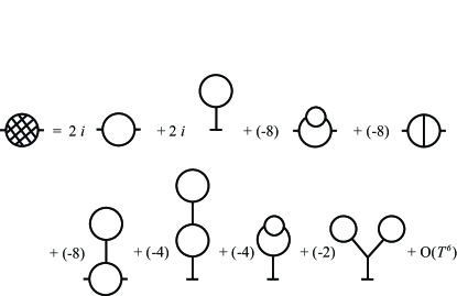
Figure 1: Feynman diagrams for the interaction self-energy $\Sigma_{n}$. Each long line corresponds to a propagator $G_{0}(\tau,\tau^{\prime})$; each vertex is associated with the interaction strength $T_{ijk}$. All internal site indices are summed and contour time variables integrated. The number in front of a graph is the factor multiplying the graph value.

So far the equations above are all exact. Several ways of approximating the nonlinear contribution to self-energy are possible. We can simply truncate the diagrams valle in the perturbative expansion for the self-energy. The diagrams for $\Sigma_{n}$ to $O(T_{ijk}^{4})$ are shown in Fig. 1. These diagrams are still in the contour variable $\tau$. For practical calculation, they have to be changed to real time $t$ in terms of $G^{\sigma\sigma^{\prime}}$ and Fourier transformed to the frequency domain. For example, the leading order contribution (first two diagrams) to the nonlinear self-energy is:

$$\!\!\!\!\!\!\Sigma^{\sigma\sigma^{\prime}}_{n,jk}[\omega]\approx 2i\!\!\sum_{lmrs}\!\!T_{jlm}T_{rsk}\!\!\int_{-\infty}^{+\infty}\!\!\!\!\!G_{0,lr}^{\sigma\sigma^{\prime}}[\omega^{\prime}]G_{0,ms}^{\sigma\sigma^{\prime}}[\omega\!-\!\omega^{\prime}]\frac{d\omega^{\prime}}{2\pi}+$$

$$\;\;\;2i\sigma\delta_{\sigma,\sigma^{\prime}}\!\!\!\!\!\!\!\!\!\sum_{lmrs,\sigma^{\prime\prime}=\pm 1}\!\!\!\!\!\!\!\!\!\sigma^{\prime\prime}T_{jkl}T_{mrs}\!\!\int_{-\infty}^{+\infty}\!\!\!\!\!\!\!G_{0,lm}^{\sigma\sigma^{\prime\prime}}[0]G_{0,rs}^{\sigma^{\prime\prime}\sigma^{\prime\prime}}[\omega^{\prime}]\frac{d\omega^{\prime}}{2\pi}.$$ (13)

Mean-field theory can be obtained by replacing $G_{0}$ by $G$, and the equations are solved iteratively.

A general program is implemented based on Eq. (5), Eq. (8) to (11), and Eq. (13). The surface Green’s function $g^{r}_{L}$ is computed using an efficient recursive method surface-green . In numerical calculation of the Green’s functions, it is important to keep a small but finite $\eta$, as the functions are singular in the limit $\eta\to 0^{+}$. In addition, on-site potentials are applied to the leads to make the system stable.

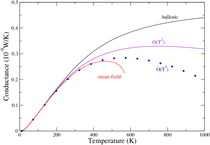
Figure 2: Thermal conductance as a function of temperature for a 1D junction with three atoms. The harmonic spring constants are $k_{L}=1.56$, $k_{R}=1.44$, $k_{C}=1.38$ (eV/(Ųamu)). The nonlinear strength is $t=1.8$ eV/(ųamu^3/2). Small onsite quadratic potentials are applied to the leads with spring constants $k_{L}^{\rm onsite}=0.01$, and $k_{R}^{\rm onsite}=0.02$ (eV/(Ųamu)).

We first test various approximations on a 1D junction with parameters comparable to that of a carbon chain. The system consists of harmonic leads and a junction part with harmonic interactions plus cubic interactions of the form $(1/3)t\sum(u_{j}-u_{j+1})^{3}$ of Fermi-Pasta-Ulam type. Figure 2 presents the results for a 3-atom junction system. We discuss the effect of nonlinearity to thermal transport. As we can see, adding nonlinear contributions suppresses the thermal conductance at high temperatures. The deviation from ballistic transport starts around 200 Kelvin. As the temperature rises further, we expect that the higher order graphs become important. The high order calculations are rather expensive, with computational complexity scaled as $O(N^{4}M^{2})$ where $N$ is system size and $M$ is sampling points in frequency. To partially take into account the higher order contributions but still keep the computation within reasonable limit for large systems, we find a mean-field theory is most satisfactory. In this version of mean-field treatment, we consider the leading diagrams of $O(T^{2})$, and replace $G_{0}$ by $G$ only for the first diagram. The equations are then solved iteratively. Good agreement with $O(T^{4})$ result is found for temperatures up to 400 K for the 1D chain. Thus we expect that the mean-field theory can give excellent results for moderately high temperatures. However, both the perturbative results and mean-field one break down at sufficiently high temperature, as the cubic nonlinearity is only metastable. To predict correctly diffusive behavior at high temperatures, the quartic interaction and higher order graphs are essential.

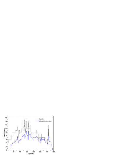
Figure 3: The ballistic transmission and the effective transmission at 300K for an (8,0) one-unit-cell carbon nanotube junction.

We now turn to the carbon nanotube junctions. The leads and the junction are of the same diameter (8,0) nanotube. The only difference is that the junction part has cubic nonlinear interactions while the leads are perfectly harmonic. The values of $T_{ijk}$ are derived from the Brenner potential by finite differences. For computational efficiency, small values of $T_{ijk}$ are truncated to zero. Figure 3 shows the ballistic transmission coefficient when the nonlinearity is set to zero, and is compared with the effective transmission due to the leading nonlinear effects (the first two graphs). It can be seen that the nonlinearity greatly suppresses the thermal transmission, particularly at low frequencies. The discontinuity is smeared out to more smooth curve due to thermal effect.

Figure 4: Thermal conductance of (8,0) carbon nanotube junction with one unit cell (0.426 nm). The inset shows the thermal conductivity as a function of tube length.

The temperature and length dependence of the nanotube thermal conductance (conductivity) is shown in Fig. 4. The mean-field theory result gives a peak in the conductance around 400K. This behavior agrees with experiments exp-papers and is in contrast with MD results which tend to give peaks at much lower temperatures md-papers . The inset shows the thermal conductivity calculated from the conductance. The cross-section is defined as $\pi d^{2}/4$, where $d$ is the diameter of the tube. If we assume that the transport up to 1 $\mu$m is still quasi-ballistic, then we can estimate that the thermal conductivity at the experimental accessible length is about 2000 W/(mK). This is qualitatively in agreement with experimental values exp-papers .

We proposed a fully quantum mechanical approach for computing heat current of solid junctions with nonlinear interactions. We have demonstrated the method with 1D and molecular junction systems. The perturbation expansion for self-energy works well up to room temperatures. However, it is still a challenge to find efficient and good approximation for the self-energy at high temperatures.

This work is supported in part by a Faculty Research Grant of the National University of Singapore.

References

- (1) R. E. Peierls, Quantum Theory of Solids, Chap. 2, (Oxford University Press, 1955).
- (2) P. Carruthers, Rev. Mod. Phys. 33, 92 (1961).
- (3) D. G. Cahill, W. K. Ford, K. E. Goodson, G. D. Mahan, A. Majumdar, H. J. Maris, R. Merlin, and S. R. Phillpot, J. Appl. Phys. 93, 793 (2003).
- (4) S. Lepri, R. Livi, and A. Politi, Phys. Rep. 377, 1 (2003).
- (5) J. Wang and J.-S. Wang, Appl. Phys. Lett, 88, 111909 (2006).
- (6) M. Michel, G. Mahler, and J. Gemmer, Phys. Rev. Lett. 95, 180602 (2005).
- (7) D. Segal, A. Nitzan, and P. Hänggi, J. Chem. Phys. 119, 6840 (2003); D. Segal and A. Nitzan, Phys. Rev. Lett. 94, 034301 (2005).
- (8) Y. Meir and N. S. Wingreen, Phys. Rev. Lett. 68, 2512 (1992); A.-P. Jauho, N. S. Wingreen, and Y. Meir, Phys. Rev. B 50, 5528 (1994).
- (9) A. Ozpineci and S. Ciraci, Phys. Rev. B 63, 125415 (2001).
- (10) N. Mingo and L. Yang, Phys. Rev. B 68, 245406 (2003).
- (11) S. Doniach and E. H. Sondheimer, Green’s Functions for Solid State Physicists, Chap. 1, (W. A. Benjamin, Reading, 1974).
- (12) L. V. Keldysh, Sov. Phys. JETP, 20, 1018 (1965).
- (13) H. Haug and A.-P. Jauho, Quantum Kinetics in Transport and Optics of Semiconductors, (Springer, Berlin, 1996).
- (14) C. Caroli, R. Combescot, P. Nozieres, and D. Saint-James, J. Phys. C 4, 916 (1971).
- (15) R. G. D. Valle and P. Procacci, Phys. Rev. B 46, 6141 (1992).
- (16) M. P. López Sancho, J. M. López Sancho, and J. Rubio, J. Phys. F: Met. Phys. 15, 851 (1985).
- (17) P. Kim, L. Shi, A. Majumdar, and P. L. McEuen, Phys. Rev. Lett. 87, 215502, (2001); E. Pop, D. Mann, Q. Wang, K. Goodson, and H. Dai, Nano Letters, 6, 96 (2006).
- (18) S. Berber, Y.-K. Kwon, and D. Tománek, Phys. Rev. Lett. 84, 4613 (2000).