Tunneling between 2D electron layers with correlated disorder: anomalous sensitivity to spin-orbit coupling

Abstract

Tunneling between two-dimensional electron layers with mutually correlated disorder potentials is studied theoretically. Due to this correlation, the diffusive eigenstates in different layers are almost orthogonal to each other. As a result, a peak in the tunnel $I$-$V$ characteristics shifts towards small bias, $V$. If the correlation in disorder potentials is complete, the peak position and width are governed by the spin-orbit coupling in the layers; this coupling lifts the orthogonality of the eigenstates. Possibility to use inter-layer tunneling for experimental determination of weak intrinsic spin-orbit splitting of the Fermi surface is discussed.

I Introduction

Knowledge of spin-orbit (SO) splitting, $\Delta$, of energy spectrum in 2D electronic systems is important for design of spintronic devices in two respects. First, a number of proposed schemes directly utilize the SO coupling for manipulating electron spin polarization by means of creating spatially inhomogeneous structures Khodas04 . Second, in proposed schemes that are not based on SO splitting, the latter limits the device performance via a SO-induced decoherence time zutic ; loss . Experimentally, large values of SO splitting can be extracted from conventional measurements, such as the beats of the Shubnikov-de Haas oscillations dorozhkin87 ; luo90 . This, however, requires that $\Delta\tau>1$, where $\tau$ is the electron scattering time. Experimental determination of $\Delta$ in the opposite limit, $\Delta\tau<1$, poses a considerable challenge. One has to look for physical effects which are anomalously sensitive to the SO-coupling. An example of such effect is the weak localization/anti-localization crossover in magnetoresistance Koga02 ; Miller03 . Tunneling measurements offer another possibility. Even when $\Delta\tau<1$, a structure related to $\Delta$ manifests itself in the $I$-$V$ characteristics, provided that the disorder is long-range, so that $\Delta\tau_{\rm tr}>1$, where $\tau_{\rm tr}$ is the transport scattering time Apalkov06 .

In 1993, Zheng and MacDonald ZM made an observation that, in the absence of the SO coupling, calculations of tunneling conductance between two parallel electron layers with short-range but correlated disorder potentials is analogous to the calculation of conductance of a single layer with long-range disorder. Formally, both calculations require solution of the equation for the vertex functions, obtained by a summation of ladder diagrams. For a single layer, the vertex function has a pole at frequency $\omega=i/\tau_{\rm tr}$, where

$$\frac{1}{\tau_{\rm tr}}=8\pi^{2}\nu\int d{\bf q}S({\bf q})\Bigl{[}1-\cos{\theta_{{\bf p},{\bf p+q}}}\Bigr{]}\delta(p^{2}-|{\bf p}+{\bf q}|^{2}),$$ (1)

where $\nu=m/2\pi$ is the 2D density of states (per spin) and $S({\bf q})$ is the Fourier component of the correlator of the intralayer disorder potential, $V({\bf r})$: $S({\bf q})=\int d{\bf r}~{}e^{-i{\bf qr}}\langle V({\bf r})V(0)\rangle$. For interlayer tunneling, the pole of the vertex function is at $\omega=i/\tau_{0}$, where $\tau_{0}$ is defined as ZM

$$\frac{1}{\tau_{\tiny{0}}}=8\pi^{2}\nu\int d{\bf q}\Bigl{[}S({\bf q})-S_{LR}({\bf q})\Bigr{]}\delta(p^{2}-|{\bf p}+{\bf q}|^{2}),$$ (2)

where similar to the above, $S_{LR}({\bf q})$ is the Fourier component of the cross-correlator $\langle V_{L}({\bf r})V_{R}(0)\rangle$ of the disorder potentials in the two layers. The physics captured by Eq. (2) is that despite strong scattering in each layer, the true eigenstates in both layers are almost identical when $V_{L}$ and $V_{R}$ are strongly correlated. Then the pole at $-i\omega=1/\tau_{0}\ll 1/\tau$ reflects the fact that eigenstates in two layers with energy difference $\gtrsim 1/\tau_{0}$ are almost orthogonal.

Basing on the above analogy, pointed out by Zheng and MacDonald, one would anticipate anomalous sensitivity of the tunneling current between two layers with short-range correlated disorder to the SO splitting in the layers. In the present paper, we will illustrate this anomalous sensitivity for a particular example of tunneling between two identical quantum wells, to which electrons are supplied by a $\delta$-layer of donors, located in the middle plane.

Figure 1: (A) Schematic illustration of a $\delta$-layer of donors located symmetrically between two identical quantum wells. SO coupling constants in the wells have equal magnitude and opposite signs; (B) Diagram describing tunneling current between two wells with correlated disorder; (C) Diagrammatic equation for the vertex function.

II Tunneling current between two 2DEG with spin-orbit interaction

The system under study is shown in Fig. 1. Once the donors get ionized by yielding their electrons to the left and right electron gases, electric fields which they create in both layers are equal in magnitude and opposite in directions. As a result, the coupling constants in the SO Hamiltonians SO of the two layers are opposite: $H^{(L)}_{\rm so}=\alpha_{\rm so}({\bf p}\times{\bm{\sigma}})_{z}$, $H^{(R)}_{\rm so}=-\alpha_{\rm so}({\bf p}\times{\bm{\sigma}})_{z}$. The important consequence of the geometry depicted in Fig. 1 is that it allows to arrange correlation between spatial wave functions in different layers drag corresponding to different energies separated by $2\Delta$. As a result, $\Delta$ manifests itself in the tunneling $I$-$V$ characteristics.

The tunneling Hamiltonian has the form,

$$H=t\sum_{\alpha}\int d^{2}r\left(\hat{\psi}^{(L)\dagger}_{\alpha}({\bf r})\hat{\psi}^{(R)}_{\alpha}({\bf r})+\hat{\psi}^{(R)\dagger}_{\alpha}({\bf r})\hat{\psi}^{(L)}_{\alpha}({\bf r})\right),$$ (3)

where $\hat{\psi}^{(L)}_{\alpha}({\bf r})$ and $\hat{\psi}^{(R)}_{\alpha}({\bf r})$ are the electron operators in the two layers, and $\alpha$ is the spin index. The overlap integral $t$ for the size-quantization wavefunctions in the two layers is assumed to be real, for simplicity. The tunneling described by Eq. (3) preserves both electron spin and momentum.

Calculation of the interlayer tunneling current (see Fig. 1) reduces to finding the vertex function for the case when the electron Green’s functions in the layers are matrices. Namely, the retarded Green’s functions are

$$\hat{G}^{(L)}_{R}(\epsilon,{\bf p})=[\epsilon-\xi-\alpha_{\rm so}({\bf p}\times{\bm{\sigma}})_{z}+i/2\tau]^{-1},$$

$$\hat{G}^{(R)}_{R}(\epsilon,{\bf p})=[\epsilon-\xi+\alpha_{\rm so}({\bf p}\times{\bm{\sigma}})_{z}+i/2\tau]^{-1},$$ (4)

where $\xi$ is the electron energy, measured from the Fermi level. Advanced Green’s functions are obtained from Eqs. (II) by reversing the sign of $i/2\tau$-terms. Solving the matrix equation illustrated in Fig. 1 yields the following generalized expression for the vertex

$${\cal T}(\omega)=t\frac{(\omega+i/\tau)^{2}-4\Delta^{2}}{(\omega+i/\tau)(\omega+i/\tau_{0})-4\Delta^{2}},$$ (5)

where $\Delta=\alpha p_{F}$, and $p_{F}$ is the Fermi momentum. In the absence of the SO coupling Eq. (5) reduces to the result ${\cal T}(\omega)=t(1-i\omega\tau)/(1-i\omega\tau_{0})$ of Ref. ZM, . Incorporating the vertex function Eq. (5) into the standard expression Mahan for the tunneling current

$$I(V) = e^{2}AtV~{}\Im\Bigl{\{}\Gamma(eV)$$ (6)

$$\times\text{Tr}\int d{\bf p}~{}{\hat{G}}^{(L)}_{R}(0,{\bf p}){\hat{G}}^{(R)}_{A}(-eV,{\bf p})\Bigr{\}},$$

we arrive to the final result,

$$I(V)=\frac{2e^{2}t^{2}A\nu V[4\Delta^{2}\tau^{-1}+(e^{2}V^{2}+\tau^{-2})\tau_{0}^{-1}]}{[e^{2}V^{2}-4\Delta^{2}-\tau^{-1}\tau_{0}^{-1}]^{2}+e^{2}V^{2}(\tau^{-1}+\tau^{-1}_{0})^{2}}.$$ (7)

Here $A$ is the lateral area.

Anomalous sensitivity of the $I$-$V$ characteristics (7) to the SO splitting is illustrated in Figs. 2-4. For large splitting, $\Delta\tau>1$ (see Fig. 2), correlation between the disorder potentials is not important. The peaks of the $I$-$V$ curves are located at $eV=\pm 2\Delta$, while the peak widths are $\approx 1/\tau$. Such a form of the $I$-$V$ curves reflects the fact that, with opposite signs the SO coupling constants in the layers, the intralayer spinor eigenfunctions are maximally correlated, when their energies differ by $2\Delta$.

Figure 2: The tunnel $I$-$V$ characteristics is plotted from Eq. (5) for different values of dimensionless scattering rate $\Delta\tau$ in the layers. For $\Delta\tau>0.5$ the current is maximal at bias $eV=2\Delta$.

As it is seen from Fig. 2, the position of the current maximum rapidly shifts from $eV=2\Delta$ towards smaller biases for $\Delta\tau\lesssim 0.5$. The $I$-$V$ characteristics for this case are shown in Fig. 3. A remarkable feature of the curves in Fig. 3 is their strong sensitivity to $\Delta$ when the disorder is strong, $\Delta\tau<1$, so that the characteristics of individual layers are insensitive to the SO coupling.

Figure 3: The tunnel $I$-$V$ characteristics is plotted from Eq. (5) for fully correlated disorder potentials in the layers at different values of $\Delta\tau\ll 1$. The current is maximal at $eV=4\Delta^{2}\tau$.

For fully correlated disorder potentials in the layers, $\tau_{0}\rightarrow\infty$, the $I$-$V$ characteristics for different values of $\Delta\tau<0.2$ fall on top of each other when plotted as a function of the ratio $eV/4\Delta^{2}\tau$. Thus, the position of maximum of the tunneling current allows to extract the Dyakonov-Perel DP spin decoherence time $\tau_{s}=(2\Delta^{2}\tau)^{-1}$. The underlying reason is that, due to opposite signs of the intralayer SO coupling constants, the eigenfunctions in the layers are not orthogonal even if disorders are fully correlated. Then $\tau_{s}^{-1}$ is a quantitative measure of the energy interval in which the orthogonality is lifted. The fact that position of the maximum in Fig. (3) is at $eV=2/\tau_{s}$ reflects that electrons in both layers undergo spin relaxation.

Incomplete correlation of disorder potentials, $V_{L}({\bf r})$ and $V_{R}({\bf r})$, in the layers is another source of lifting of orthogonality of eigenstates. This mechanism is quantified by the energy scale $1/\tau_{0}$, defined by Eq. (2). It might be expected that in the presence of both mechanisms the maximum is located at $eV=2/\tau_{s}+1/\tau_{0}$, which has a meaning of a combined dephasing time. This is indeed the case, as illustrated in Fig. 4.

III Effect of electron-electron interactions

Let us address the question whether the above SO-induced peaks survive the presence of electron-electron interactions. Interactions cause a dynamic lifting of orthogonality of the eigenstates, and might result in the broadening of the peaks. We now demonstrate that at zero temperature the peaks are robust, but eventually get smeared away as the temperature increases.

Figure 4: $I$-$V$ curves for different values of spin-orbit coupling and different degrees of correlation of disorder in the layers. The maxima are at biases determined by the combined decoherence rate. The latter is dominated by $1/\tau_{0}$ term for $\Delta\tau=0.05$ and by spin relaxation term, $4\Delta^{2}\tau$, for $\Delta\tau=0.4$.

On the quantitative level, in order to incorporate both the interactions and the correlated disorder into the theory, it is convenient to express the tunneling current in terms of the exact eigenfunctions, which are the same in the two layers. Let us denote with $\psi_{m}({\bf r})$ the $m$-th eigenstate for a given realization of disorder potential. The energy of this state is equal to $\epsilon_{m}$ as electron-electron interactions are neglected. In the presence of electron-electron interactions the retarded electron Green function can be written as,

$$G_{R}(\epsilon,{\bf r}_{1},{\bf r}_{2})=\sum_{m}\frac{\psi_{m}({\bf r}_{1})\psi_{m}^{\dagger}({\bf r}_{2})}{\epsilon-\epsilon_{m}-\Sigma_{m}(\epsilon)},$$ (8)

where $\Sigma_{m}(\epsilon)$ denotes the electron self-energy of the $m$-th eigenstate.

The knowledge of the eigenfunctions suffices to evaluate the tunneling current (in the lowest order in $t$) in a general form,

$$I(V)=2et^{2}\int\frac{d\epsilon}{2\pi}\Bigl{[}n(\epsilon)-n(\epsilon+eV)\Bigr{]}$$

$$\times\int d{\bf r}_{1}d{\bf r}_{2}{\cal A}^{(L)}(\epsilon,{\bf r}_{1},{\bf r}_{2}){\cal A}^{(R)}(\epsilon+eV,{\bf r}_{2},{\bf r}_{1}),$$ (9)

and express it via the Fermi-Dirac distribution $n(\epsilon)$ and the non-averaged spectral functions in the left and right layers, ${\cal A}^{(L)}(\epsilon,{\bf r}_{1},{\bf r}_{2})$ and ${\cal A}^{(R)}(\epsilon,{\bf r}_{1},{\bf r}_{2})$, respectively. The spectral function is determined by the difference of the retarded and advanced functions in each layer,

$${\cal A}(\epsilon,{\bf r}_{1},{\bf r}_{2})=\frac{i}{2}\Bigr{[}G_{R}(\epsilon,{\bf r}_{1},{\bf r}_{2})-G_{A}(\epsilon,{\bf r}_{1},{\bf r}_{2})\Bigl{]}.$$ (10)

At this point, we emphasize that, for fully correlated disorder (neglecting spin-orbit interaction), we can perform coordinate integration in Eq. (III) prior to performing the configuration averaging, and cast it in the form

$$I(V)=2et^{2}\sum_{m}\int\limits_{-eV}^{0}\frac{d\epsilon}{2\pi}~{}\Im\left[\frac{1}{\epsilon-\epsilon_{m}-\Sigma_{m}(\epsilon)}\right]$$

$$\times\Im\left[\frac{1}{\epsilon+eV-\epsilon_{m}-\Sigma_{m}(\epsilon+eV)}\right].$$ (11)

The reason why explicit integrations over ${\bf r}_{1}$ and ${\bf r}_{2}$ can be performed in Eq. (III), leading to Eq. (III), is the mutual orthogonality of the eigenstates in the two layers resulting from the fully correlated disorder. In Eq. (III) we have also set $T=0$ in the difference of the Fermi functions. This is justified as long as $T$ is much smaller than $E_{F}$. The reason is that, similarly to the in-plane conduction, the temperature dependence of the tunnel current comes exclusively from the $T$-dependence of the self-energy, i.e. from inelastic processes.

The question whether $\Sigma_{m}(\epsilon)$ and $\Sigma_{m}(\epsilon+eV)$ in Eq. (III) can be replaced by the disorder averaged values is highly non-trivial in the limit $T\to 0$. However, we can rigorously address the issue of smearing of the SO-related peak in the $I$-$V$ curve for disordered layer by treating interactions at the perturbative level, which corresponds to the expansion of Eq. (III) to the first order in $\Sigma_{m}$. This expansion yields,

$$\delta I(V)=\frac{2t^{2}\nu A}{eV^{2}}\int\limits_{0}^{eV}d\epsilon\Bigl{[}\gamma_{\epsilon}(\epsilon+eV)+\gamma_{\epsilon+eV}(\epsilon)\Bigr{]},$$ (12)

where $\gamma_{\epsilon}(\omega)=\nu^{-1}\sum_{m}\langle\delta(\epsilon-\epsilon_{m})~{}\Im\Sigma_{m}(\omega)\rangle$ is now the disorder-averaged inverse inelastic lifetime.

(i) For $\Delta\tau\ll 1$ the peak position, $eV=4\Delta^{2}\tau$, is below the elastic scattering rate, i.e. at the energy corresponding to the peak position the motion of electrons is diffusive. The corresponding lifetime was studied in the seminal paper Ref. Abrahams, , and was shown to be, $\gamma(\epsilon)\sim|\epsilon|/E_{F}\tau$. We can now compare Eq. (12) with the “non-interacting” value of current, given by Eq. (7), at the bias corresponding to the peak position, $eV=4\Delta^{2}\tau$. We find that the ratio $\delta I/I\sim 1/E_{F}\tau$ is small regardless of the actual value of the decoherence rate.

(ii) Similarly, for large values of spin-orbit splitting, $\Delta\tau\gg 1$, we should utilize ballistic inverse lifetime, $\gamma(\epsilon)=(\epsilon^{2}/4\pi E_{F})\ln{[E_{F}/\epsilon]}$, established in Refs. MJ, ; ZDS, . Comparison of Eq. (12) with the value given by Eq. (7) at the peak position, $eV=2\Delta$, we conclude that the corresponding ratio is again small, $\delta I/I\sim(1/E_{F}\tau)\ln{[E_{F}/\Delta]}$.

This suggests that, at zero temperature, interactions do not destroy the SO-induced peak in the $I$-$V$ curve. However, this destruction eventually happens upon increasing $T$. A crude estimate for the temperature at which the peak is washed out by interactions can be obtained by equating the peak position $eV=4\Delta^{2}\tau$ to $\gamma(\epsilon=T)$. With logarithmic accuracy, this yields the restriction $T<(\Delta\tau)^{2}E_{F}$, so that even with $\Delta\tau<1$ the peak survives at reasonably high temperatures.

To trace quantitatively the smearing of the peak with $T$, we first note that “single-electron” $I$-$V$ characteristics (7) can be obtained from Eq. (III) upon inserting spin decoherence rate into the self-energy, $\Sigma_{m}\to 2i\Delta^{2}\tau$, and replacing the sum over $\epsilon_{m}\to\xi$ by the integral, $\sum_{m}\to\nu A\int d\xi$. As the next step, we take into account the finite-$T$ decoherence by writing $\Sigma=2i\Delta^{2}\tau+i\gamma_{T}$, where $\gamma_{T}=(T/2E_{F}\tau)\ln{(T_{1}/T)}$ Abrahams ; Blanter and $T_{1}=r_{s}^{2}E_{F}^{4}\tau^{3}$; here $r_{s}$ is the interaction parameter of 2D electron gas. To utilize the energy-independent $\gamma(T)$ in the self-energy, the temperature must be large compared to the peak position, $eV=2\Delta^{2}\tau$. This requirement does not contradict the restriction on the smearing obtained from the above crude estimate. Indeed, both conditions can be conveniently rewritten as, $T/E_{F}\tau\ll\Delta^{2}\tau\ll T$, so that it is the large value of $E_{F}\tau$ which makes them consistent. Upon the suggested replacements, the temperature-dependent $I$-$V$ characteristics follows from Eq. (7) with the spin relaxation rate modifies as $2\Delta^{2}\tau\to 2\Delta^{2}\tau+\gamma_{T}$, with $\tau_{0}=\infty$

$$I(V)=4e^{2}t^{2}A\nu\frac{V(2\Delta^{2}\tau+\gamma_{T})}{e^{2}V^{2}+4(2\Delta^{2}\tau+\gamma_{T})^{2}}.$$ (13)

Eq. (13) indicates that the position of maximum of the $I$-$V$ curve shifts almost linearly with temperature, see Fig. 5. This suggests that the SO relaxation rate can be inferred from experiment even when measurements are performed at $T>(\Delta\tau)^{2}E_{F}$. One has to plot the peak position as a function of $T$ and extrapolate the data to $T\rightarrow 0$. Besides, the actual restriction on $T$ is “softer” than the one obtained from the crude estimate, by virtue of numerical coefficients in $\gamma_{T}$ and spin relaxation time $1/\tau_{s}$. Indeed, the requirement $\gamma_{T}\tau_{s}/2<1$ imposes (neglecting logarithmic factor) the following restriction, $T<4(\Delta\tau)^{2}E_{F}$.

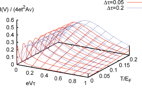
Figure 5: (Color online) Temperature dependence of the tunneling characteristics for different values of spin-orbit coupling constant and fully correlated disorder, from Eq. (13). Increasing $T$ results in the broadening of the peak and its net shift towards higher biases.

IV Summary and Conclusions

Our main finding is that, with correlated disorder in the layers, the SO coupling causes a zero in $dI/dV$ even for $\Delta\tau\ll 1$, when the spin subbands in the layers are not resolved. For clean layers with $\Delta\tau>1$, sensitivity of tunneling current to the SO coupling was pointed out in Ref. RaichevDebray, .

The condition that position of zero in $dI/dV$ is due to the SO coupling is that the contribution, $4\Delta^{2}\tau$, to the combined decoherence rate exceeds $1/\tau_{0}$, caused by incomplete correlation of disorders in the layers. To estimate the feasibility to meet this condition, we assume that the origin of incomplete correlation is a finite width, $a$, of the $\delta$-layer, see Fig. 1. Assuming that the in-plane positions of donors with concentration, $N_{d}$, are completely random, the Fourier components of the correlators, entering the expression Eq. (2) for $\tau_{0}^{-1}$, can be presented as $S_{LR}({\bf q})=N_{d}|U({\bf q})|^{2}e^{-qd}$; $S({\bf q})=N_{d}|U({\bf q})|^{2}\sinh{(qa)}~{}e^{-qd}/qa$, where $d$ is the barrier thickness, and $U({\bf q})$ is the Fourier transform of the potential created by a donor in the layer. Then Eq. (2) takes the form

$$\frac{1}{\tau_{0}}=2\pi\nu N_{d}\int d{\bf q}~{}|U({\bf q})|^{2}\left(\frac{\sinh{qa}}{qa}-1\right)~{}e^{-qd}.$$ (14)

Assuming that the screening radius in the layers is smaller than $d$, we can set $U(1/d)\approx U(0)$. Then Eq. (14) yields $\tau_{0}/\tau=(a/d)^{2}$, so that the condition $4\Delta^{2}\tau>\tau_{0}^{-1}$ reduces to $\Delta\tau>a/2d$, i.e. the value $\Delta\tau=0.05$, used in the numerics above, is quite feasible for the atomically sharp $\delta$-layer.

As a final remark, the assumption, crucial for our calculations, was that the barrier is spatially homogeneous, so that the tunneling occurs with the conservation of the in-plane momentum. We had also assumed that the positions of donors in the $\delta$-layer are random. This randomness might, in principle, lift the momentum conservation. The condition that the effect of randomness is negligible is that the tunneling-induced splitting, $t$, of the states in the layers is the smallest scale in the problem. In fact, we had used this condition by restricting the calculations to the lowest order in $t$. Under this condition, the under-barrier scattering of the tunneling electron by donors in the classically forbidden region is exponentially suppressed as compared to the situation when donors are located in the vicinity of the layers.

- (1) M. Governale and U. Zülicke, Phys. Rev. B 66, 073311 (2002); V. M. Ramaglia, et. al., Eur. Phys. J. B 36, 365 (2003); M. Khodas, A. Shekhter, and A. M. Finkel’stein, Phys. Rev. Lett. 92, 086602 (2004); G. Usaj and C. A. Balseiro, Phys. Rev. B 70, 041301(R) (2004), A. O. Govorov, A. V. Kalameitsev, and J. P. Dulka, Phys. Rev. B 70, 245310 (2004); P. G. Silvestrov and E. G. Mishchenko, cond-mat/0506516.
- (2) I. Zutic, J. Fabian, and S. Das Sarma, Rev. Mod. Phys. 76, 323 (2004).
- (3) V. Cerletti, W. A. Coish, O. Gywat, and D. Loss, Nanotechnology 16, R27 (2005).
- (4) S. I. Dorozhkin and E. B. Ol’shanetskii, JETP Lett. 46, 502 (1987).
- (5) J. Luo, H. Munekata, F. F. Fang, and P. J. Stiles, Phys. Rev. B 38, 10 142 (1988); Phys. Rev. B 41, 7685 (1990).
- (6) T. Koga, J. Nitta, T. Akazaki, and H. Takayanagi, Phys. Rev. Lett. 89, 046801 (2002).
- (7) J. B. Miller, D. M. Zumbuhl, C. M. Marcus, Y. B. Lyanda-Geller, D. Goldhaber-Gordon, K. Campman, and A. C. Gossard, Phys. Rev. Lett. 90, 076807 (2003).
- (8) V. M. Apalkov and M. E. Raikh, Phys. Rev. Lett. 89, 096805 (2002); V. M. Apalkov, M. E. Raikh, and B. Shapiro, Phys. Rev. B 73, 125339 (2006).
- (9) L. Zheng and A. H. MacDonald, Phys. Rev. B 47, 10619 (1993).
- (10) Yu. A. Bychkov and E. I. Rashba, JETP Lett. 39, 78 (1984).
- (11) Previously this correlation was discussed in I. V. Gornyi, A. G. Yashenkin, and D. V. Khveshchenko, Phys. Rev. Lett. 83, 152 (1999), in connection with Coulomb drag between the layers.
- (12) G. D. Mahan, in Many-Particle Physics (Plenum, New York, 1981).
- (13) M. I. Dyakonov and V. I. Perel, Sov. Phys. JETP 33, 467 (1971).
- (14) E. Abrahams, P. W. Anderson, P. A. Lee, and T. V. Ramakrishnan, Phys. Rev. B 24, 6783 (1981).
- (15) T. Jungwirth and A. H. MacDonald, Phys. Rev. B 53, 7403 (1996).
- (16) L. Zheng and S. Das Sarma, Phys. Rev. B 53, 9964 (1996).
- (17) Ya. M. Blanter, Phys. Rev. B 54, 12807 (1996).
- (18) O. E. Raichev and P. Debray, Phys. Rev. B 67, 155304 (2004).