Critical behavior of the three- and ten-state short-range Potts glass:
A Monte Carlo study

Abstract

We study the critical behavior of the short-range $p$-state Potts spin glass in three and four dimensions using Monte Carlo simulations. In three dimensions, for $p=3$, a finite-size scaling analysis of the correlation length shows clear evidence of a transition to a spin-glass phase at $T_{\rm c}\simeq 0.273$ for a Gaussian distribution of interactions and $T_{\rm c}\simeq 0.377$ for a $\pm J$ (bimodal) distribution. These results indicate that the lower critical dimension of the three-state Potts glass is below three. By contrast, the correlation length of the ten-state ($p=10$) Potts glass in three dimensions remains small even at very low temperatures and thus shows no sign of a transition. In four dimensions we find that the $p=3$ Potts glass with Gaussian interactions has a spin-glass transition at $T_{\rm c}\simeq 0.536$.

I Introduction

There are two main motivation for studying the Potts glass: First, the model for which the number of Potts states $p$ is equal to $3$ is a model for orientational glassesBinder and Reger (1992) (also known as quadrupolar glasses), which are randomly diluted molecular crystals where quadrupolar moments freeze in random orientations upon lowering the temperature due to randomness and competing interactions. This is similar to spin glasses where spins are frozen in random directions in the spin-glass phase. However, unlike conventional spin-glass systemsBinder and Young (1986) with Ising or vector spins, the Potts model does not have spin inversion symmetry, except for the special case with $p=2$ in which case the Potts model reduces to the Ising model. In mean-field theory (i.e., for the infinite-range version of the model) it is foundGross et al. (1985) that the three-state Potts glass has a finite transition temperature to a spin-glass-like phase.

Second, the Potts glass could help us understand the structural glass transition of supercooled fluids. In the mean-field (i.e., infinite-range) limit, the Potts glass with $p>4$ has a behavior quite different from that of the Ising spin glass since twoKirkpatrick and Wolynes (1987); Kirkpatrick and Thirumalai (1988) transitions occur in the Potts case. As temperature is lowered, the first transition is a dynamical transition at $T_{\rm d}$ below which the autocorrelation functions of the Potts spins do not decay to zero in the long-time limit. The second transition is a static transition at $T_{\rm c}<T_{\rm d}$ where a static order parameter, described by “one-step replica symmetry breaking,” appears discontinuously. At the mean-field level, it turns out that the the equations which describe the dynamics of the $p$-spin Potts glass for $T>T_{\rm d}$ are almost identical to the the mode-coupling equations; see Ref. Götze and Sjögren, 1992 and references therein, which describe structural glasses as they are cooled towards the glass transition. Hence Potts glasses with $p>4$ and structural glasses seem to be connected, at least in mean-field theory.

However, it is important to understand to what extent these predictions for phase transitions in the infinite-range Potts glass are also valid for more realistic short-range models. Here we consider this question by performing Monte Carlo simulations on the three-state and ten-state Potts glass models.

Earlier work on short-range three-state Potts glasses in three dimensions have used zero-temperature domain-wall renormalization group methods,Banavar and Cieplak (1989a, b) Monte Carlo simulations,Scheucher et al. (1990); Scheucher and Reger (1992); Reuhl et al. (1998) and high temperature series expansions.Singh (1991); Schreider and Reger (1995); Lobe et al. (1999) The results of the domain-wall and Monte Carlo studies have generally indicated that the lower critical dimension $d_{l}$ is equal to, or close to, $3$. The series expansion results tend to be better behaved in higher dimensions and less reliable in $d=3$, but Schreider and RegerSchreider and Reger (1995) have also argued in favor of $d_{l}=3$ from an analysis of their series. Overall, though, it seems to us that conclusive evidence for the value of the lower critical dimension is still lacking. In this paper we therefore investigate the lower critical dimension of the three-state Potts glass by Monte Carlo simulations of this model in three space dimensions using the method that has been most successful in elucidating the phase transition in IsingBallesteros et al. (2000) as well as vectorLee and Young (2003) spin glasses: a finite-size scaling analysis of the finite-size correlation length.

In four space dimensions, Scheucher and RegerScheucher and Reger (1993) performed Monte Carlo simulations, finding that the critical temperature $T_{\rm c}$ is finite and a value for the order parameter exponent $\beta$ close to zero, as well as a correlation length exponent $\nu$ consistent with $1/2$. These are the expectedGross et al. (1985) values at the discontinuous transition in the mean-field Potts model for $p>4$. It is surprising that these should be found in four dimensions, since, as for Ising and vector spin glasses,Harris et al. (1976) the upper critical dimension is $6$. To try to clarify this situation we therefore also apply the finite-size scaling analysis of the correlation length to the three-state Potts glass in $d=4$.

Earlier work on the ten-state Potts glass in three dimensions by Brangian et al.Brangian et al. (2002a); Brangian et al. (2003) found that, in contrast to the mean-field version of the same model, both the static and dynamic transitions are wiped out. Relaxation times follow simple Arrhenius behavior, and judging by the lack of size dependence in the results, the correlation length is presumed to be small, although it was not calculated explicitly. In this paper we calculate the correlation length and find that it is always less than one lattice spacing, consistent with the results of Brangian et al.

In Sec. II we discuss the model and the numerical method that we have used. We show the results of the simulations for the three-state model in Sec. III and for the ten-state model in Sec. IV. Section V contains a summary.

II Model and method

In the Potts glass, the Potts spin on each site $i$ can be in one of $p$ different states, $n_{i}=1,2,\ldots,p$. If neighboring spins at $i$ and $j$ are in the same state, the energy is $-J_{ij}$, whereas if they are in different states, the energy is zero. Thus the Hamiltonian of the model is given by

$${\mathcal{H}}=-\sum_{\langle i,j\rangle}J_{ij}\delta_{{n_{i}}{n_{j}}}\,,$$ (1)

in which the summation is over nearest-neighbor pairs. The sites lie on a hypercubic lattice with $N=L^{d}$ sites, and we consider dimensions $d=3$ and $4$. The interactions $J_{ij}$ are independent random variables with either a Gaussian distribution with mean $J_{0}$ and standard deviation unity,

$${\mathcal{P}}(J_{ij})=\frac{1}{\sqrt{2\pi}}e^{-(J_{ij}-J_{0})^{2}/2},$$ (2)

or a bimodal ($\pm J$) distribution with zero mean,

$${\cal P}(J_{ij})=\frac{1}{2}\left[\delta(J_{ij}-1)+\delta(J_{ij}+1)\right].$$ (3)

It is convenient to rewrite the Potts glass Hamiltonian using the “simplex” representation where the $p$ states are mapped to the $p$ corners of a hypertetrahedron in $(p-1)$-dimensional space. The state at each site is represented by a $(p-1)$-dimensional unit vector $\mathbf{S}_{i}$, which takes one of $p$ values, $\mathbf{S}^{\lambda}$ satisfying

$$\mathbf{S}^{\lambda}\cdot\mathbf{S}^{\lambda^{\prime}}=\frac{p\;\delta_{\lambda\lambda^{\prime}}-1}{p-1}$$ (4)

($\lambda=1,2,\cdots,p$). In the simplex representation, the Potts Hamiltonian is similar to a $(p-1)$-component vector spin-glass model,

$${\mathcal{H}}=-\sum_{\langle i,j\rangle}J^{\prime}_{ij}\mathbf{S}_{i}\cdot\mathbf{S}_{j},$$ (5)

ignoring an additive constant, where

$$J^{\prime}_{ij}=\frac{(p-1)}{p}J_{ij}.$$ (6)

However, an important difference compared with a vector spin glass is that, except for $p=2$, if $\mathbf{S}^{\lambda}$ is one of the (discrete) allowed vectors, then its inverse $-\mathbf{S}^{\lambda}$ is not allowed.

In mean-field theory, assuming the transition is continuous, the spin-glass transition temperature is given byGross et al. (1985)

$$T_{\rm c}^{\rm MF}=\frac{z^{1/2}}{p}[(J_{ij}-J_{0})^{2}]_{\mathrm{av}}^{1/2}=\frac{z^{1/2}}{p}=\frac{z^{1/2}}{p-1}[(J^{\prime}_{ij}-J_{0}^{\prime})^{2}]_{\mathrm{av}}^{1/2},$$ (7)

where $z=2d$ is the number of nearest neighbors and $[\cdots]_{\mathrm{av}}$ denotes an average over disorder. Actually, in mean-field theory there is a discontinuity in the order parameter for $p>4$ and the transition then occurs at a higher temperature.Gross et al. (1985) For the case of $p=10$ this is found to be atBrangian et al. (2002b) $T_{\rm c}=0.28$, rather than Eq. (7), which predicts $T_{\rm c}=0.24$. Hence, the mean-field transition temperatures for the models discussed in this paper are

$$T_{\rm c}^{\rm MF}=\left\{\begin{array}[]{lll}0.82&&\mbox{three-state},\;d=3,\\ 0.94&&\mbox{three-state},\;d=4,\\ 0.28&&\mbox{ten-state},\;d=3.\end{array}\right.$$ (8)

The spin-glass order parameter for a Potts spin glass with wave vector ${\bf k}$, $q^{\mu\nu}({\bf k})$, is defined to be

$$q^{\mu\nu}({\bf k})=\frac{1}{N}\sum_{i}S_{i}^{\mu(1)}S_{i}^{\nu(2)}e^{i{\bf k}\cdot{\bf R}_{i}},$$ (9)

where $\mu$ and $\nu$ are components of the spin in the simplex representation and “$(1)$” and “$(2)$” denote two identical copies (replicas) of the system with the same disorder. The wave-vector-dependent spin-glass susceptibility $\chi_{\rm SG}({\bf k})$ is then given by

$$\chi_{\rm SG}({\bf k})=N\sum_{\mu,\nu}[\langle\left|q^{\mu\nu}({\bf k})\right|^{2}\rangle]_{\mathrm{av}},$$ (10)

where $\langle\cdots\rangle$ denotes a thermal average.

The correlation length, $\xi_{L}$, of a system of size $L$ is definedBallesteros et al. (2000) by

$$\xi_{L}=\frac{1}{2\sin(k_{\mathrm{min}}/2)}\left[\frac{\chi_{\rm SG}({\bf 0})}{\chi_{\rm SG}({\bf k}_{\mathrm{min}})}-1\right]^{1/2},$$ (11)

where ${\bf k}_{\mathrm{min}}=(2\pi/L,0,0)$ is the smallest nonzero wave vector. Since the ratio of $\xi_{L}/L$ is dimensionless, it satisfies the finite-size scaling form

$$\frac{\xi_{L}}{L}=\widetilde{X}\left(L^{1/\nu}[T-T_{\rm c}]\right),$$ (12)

where $\nu$ is the correlation length exponent, $T_{\rm c}$ is the transition temperature, and $\widetilde{X}$ a scaling function. At the transition temperature, $\xi_{L}/L$ is independent of $L$, and so this quantity is particularly convenient for locating the transition. Once $T_{\rm c}$ has been obtained from the intersection point, one determines the exponent $\nu$ by requiring that the data collapse onto a single curve when plotted as a function of $L^{1/\nu}(T-T_{\rm c})$.

We are also interested in obtaining the critical exponent $\eta$ which characterizes the power-law decay of the correlation function at criticality. The two exponents $\nu$ and $\eta$ completely characterize the critical behavior, since the other exponents can be obtained from them using scaling relations.Yeomans (1992) From scaling theory, we expect the spin-glass susceptibility $\chi_{\rm SG}$ to vary as

$$\chi_{\rm SG}=L^{(2-\eta)}\widetilde{C}\left(L^{1/\nu}[T-T_{\rm c}]\right).$$ (13)

To perform the scaling fits systematically, we use the method recently proposed in Ref. Katzgraber et al., 2006. By assuming that the scaling function can be approximated in the vicinity of the critical temperature by a third-order polynomial (with coefficients $c_{i}$, $i$=1–4), a nonlinear fit can be performed on the data for $\xi_{L}$ with six parameters ($c_{i}$, $T_{\rm c}$, and $\nu$) using Eq. (12) in order to determine the optimal finite-size scaling. For the $\chi_{\rm SG}$ data, we have an additional parameter $\eta$ from Eq. (13), so the fit involves 7 parameters. It is necessary to choose a temperature range within the scaling region to do the fits. We limit our temperature range to where results from scaling the data in $(T-T_{\rm c})$ and $(\beta-\beta_{\rm c})$, where $\beta=1/T$ is the inverse temperature, agree within error bars and quote the results obtained from the fits with $(T-T_{\rm c})$. To estimate the errors we used a bootstrap procedure, described in Ref. Katzgraber et al., 2006. If there are $N_{\rm samp}$ samples for a given size, we generate $N_{\rm boot}=100$ random sets of the samples (with replacement) with $N_{\rm samp}$ samples in each set, do the analysis for each set, and take the standard deviation of the results from the sets to be the error. We emphasize that this gives the statistical errors only. In addition, there can be systematic errors, from corrections to finite-size scaling which are difficult to estimate from simulations on only a modest range of sizes, as is possible here.

Spin-glass simulations are hampered by long equilibration times, so we use parallel tempering,Hukushima and Nemoto (1996); Marinari (1998) which has proven useful in speeding up equilibration. In this approach, copies of the system with the same interactions are simulated at several temperatures. To check for equilibration, we use the following relation which holds if the couplings $J_{ij}$ are drawn from a Gaussian distribution with mean $J_{0}$ and unit standard deviation:

$$\frac{2T[U]_{\mathrm{av}}}{z}=\left[\langle\delta_{n_{i}n_{j}}\rangle^{2}\right]_{\mathrm{av}}-\left[\langle\,(\delta_{n_{i}n_{j}})^{2}\,\rangle\right]_{\mathrm{av}}-J_{0}T\left[\langle\delta_{n_{i}n_{j}}\rangle\right]_{\mathrm{av}},$$ (14)

where $U=(1/N)\langle{\mathcal{H}}\rangle$ is the energy per spin for a given disorder realization. Equation (14) is obtainedKatzgraber et al. (2001) by integrating by parts the expression for the energy with respect to the interactions $J_{ij}$. Note that the square can be omitted in the second term on the right of Eq. (14) (since $\delta_{n_{i}n_{j}}$ only takes values 1 and 0). The first term on the right is calculated from two copies at the same temperature—i.e., $\left[\langle\delta_{n_{i}n_{j}}\rangle^{(1)}\langle\delta_{n_{i}n_{j}}\rangle^{(2)}\right]_{\mathrm{av}}$. Hence, if $N_{T}$ is the number of temperatures, the total number of copies simulated (with the same interactions) is $2N_{T}$. As the simulation proceeds, the left-hand side (LHS) of Eq. (14) approaches the equilibrium value from above, while the right-hand side (RHS) approaches the (same) equilibrium value from below since the spins in the two copies are initially uncorrelated. When both quantities are simultaneously plotted as a function of Monte Carlo sweeps, the two curves merge when equilibration is reached and remain together subsequently.Katzgraber et al. (2001) Hence requiring that Eq. (14) is satisfied is a useful test for equilibration.

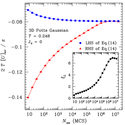
Figure 1: (Color online) An equilibration plot showing the left-hand side (upper curve) and right-hand side (lower curve) of Eq. (14). The data are for the three-state Potts glass in $d=3$ for $L=12$ at $T=0.248$ as a function of equilibration time measured in Monte Carlo sweeps, $N_{\rm sw}$. An equal number of sweeps are also performed for measurement, so the total number of sweeps is $2N_{\rm sw}$, respectively. The two sets of data merge at long times, as expected, and then remain independent of time. The inset shows the correlation length $\xi_{L}$ for the corresponding number of Monte Carlo sweeps.

An example of the equilibration test is shown in Fig. 1 for the three-state Potts glass in $d=3$ for $L=12$ at $T=0.248$. In the main panel, the upper curve is the energy term on the left-hand side of Eq. (14) while the lower curve corresponds to the right-hand side of Eq. (14) as a function of equilibration time measured in Monte Carlo sweeps (MCS). Note that one sweep consists of one Metropolis sweep of single spin-flip moves on each copy, followed by a sweep of global moves in which spin configurations at neighboring temperatures are swapped. Figure 1 shows the number of sweeps used for measurements, $N_{{}_{\textrm{\scriptsize sw}}}$; in addition, an equal number of sweeps have been used for equilibration, so the total number of sweeps is $2N_{{}_{\textrm{\scriptsize sw}}}$. We see that the two curves merge in this case at around $10^{7}$ MCS and stay within error bars after that, indicating that equilibration has been reached. The inset of Fig. 1 shows the correlation length $\xi_{L}$ as a function of Monte Carlo sweeps. The data increase until $\sim 10^{7}$ MCS where they saturate. This indicates that the equilibration time for the correlation length is in agreement with the equilibration time determined from the requirement that the two sides of Eq. (14) agree.

Unfortunately, the equilibration test using Eq. (14) only works for a Gaussian bond distribution. For the bimodal disorder distribution, we study how the results vary when the simulation time is successively increased by factors of 2 (logarithmic binning of the data). We require that the last three measurements for all observables agree within error bars.

For the Potts glass with $p>2$, an additional issue arises, which is not present for the Ising ($p=2$) case: At low temperatures ferromagnetic correlations developElderfield and Sherrington (1983) due to lack of spin-inversion symmetry, even for a symmetric disorder distribution ($J_{0}=0)$. Since we want to study the glassy phase, rather than the ferromagnetic phase, we can mitigate this undesirable feature by choosing a negative value for $J_{0}$. A choice of $J_{0}=-1$ seems sufficient for the ten-state Potts glass,Brangian et al. (2003) while for the three-state Potts glass, the ferromagnetic correlations are small, as we shall show, so we set $J_{0}=0$.

III Three-state Potts glass

III.1 Gaussian disorder ($\boldsymbol{d=3}$)

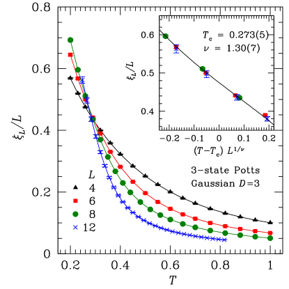
Figure 2: (Color online) Finite-size correlation length $\xi_{L}/L$ vs $T$ for the three-state Potts glass with Gaussian couplings in three dimensions. The curves intersect at $T_{\rm c}\simeq 0.273$. The inset shows a scaling plot according to Eq. (12) using $T_{\rm c}=0.273$ and $\nu=1.30$. The solid line is the third-order polynomial used in the fit.

We first discuss results for the three-state Potts glass with Gaussian interactions. The simulation parameters are shown in Table. 1. As shown in Fig. 2, the data for $\xi_{L}/L$ intersect at $T\simeq 0.27$. The common intersection provides good evidence for a spin-glass transition at this temperature. It would be desirable to obtain data in this temperature range for larger sizes, but unfortunately equilibration times are prohibitively long. Interestingly, the same transition temperature $T_{\rm c}\simeq 0.27$ was proposed earlier by Banavar and CieplakBanavar and Cieplak (1989a, b) who studied the free-energy sensitivity to changes in boundary conditions at finite temperature using very small system sizes $L=2$ and 3.

To determine $T_{\rm c}$ and $\nu$, we analyze the $\xi_{L}$ data for $L\geq 6$ using the method discussed in Sec. II for the temperature range $0.20<T<0.32$ for all $L$ and obtain

$$T_{\rm c}=0.273(5),\qquad\nu=1.30(7)\,.$$ (15)

A finite-size scaling analysis of $\xi_{L}/L$ according to Eq. (12) is shown in the inset of Fig. 2 for $L\geq 6$. The solid line represents the third-order polynomial that we have used to approximate the scaling function. The data collapse well.

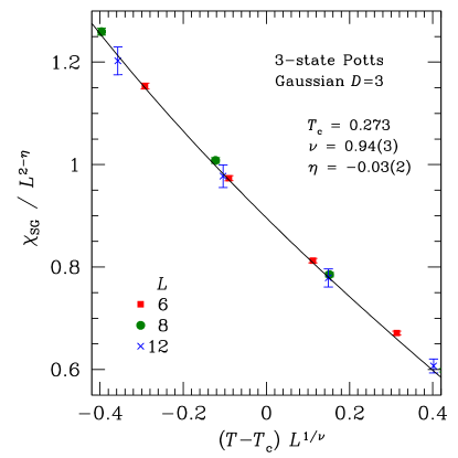
Figure 3: (Color online) Scaling plot of $\chi_{\rm SG}/L^{2-\eta}$ vs $T$ for the three-state Potts glass with Gaussian interactions in three dimensions according to Eq. (13) with $T_{\rm c}$ fixed to 0.273 (determined from the data for $\xi_{L}/L$ shown in Fig. 2). The fit to Eq. (13) then gives $\eta=-0.03$ and $\nu=0.94$.

Table 1: Parameters of the simulation for the three-state Potts glass with Gaussian interactions and $J_{0}=0$ in three dimensions. $N_{{}_{\textrm{\scriptsize samp}}}$ is the number of samples. $N_{{}_{\textrm{\scriptsize sw}}}$ is the total number of Monte Carlo sweeps used for measurement for each of the $2N_{T}$ replicas for a single sample. An equal number of sweeps is used for equilibration; hence, the total number of MCS performed is $2N_{{}_{\textrm{\scriptsize sw}}}$. $T_{{}_{\textrm{\scriptsize min}}}$ is the lowest temperature simulated, and $N_{T}$ is the number of temperatures used in the parallel tempering method for each system size $L$.

$L$	$T_{\mbox{\footnotesize min}}$	$N_{T}$	$N_{\mbox{\footnotesize samp}}$	$N_{\mbox{\footnotesize sw}}$
4	0.2	18	9356	80000
6	0.2	18	3980	80000
8	0.2	20	4052	655360
12	0.248	28	352	16777216

Next we discuss the results for $\chi_{\rm SG}$. We find that allowing $T_{\rm c}$ to vary, in addition to $\nu$ and $\eta$, the value of $T_{\rm c}$ so obtained is rather different from that obtained using data for $\xi_{L}/L$. Since we believe the value of $T_{\rm c}$ obtained from $\xi_{L}/L$—namely, $T_{\rm c}=0.273$—to be our most accurate estimate, we fix $T_{\rm c}$ to this value and fit $\eta$ and $\nu$ (and the polynomial parameters $c_{i}$) to Eq. (13). This gives $\nu=0.94(3)$ and

$$\eta=-0.03(2)\,.$$ (16)

We show the corresponding plot in Fig. 3.

If we analyze $\chi_{\rm SG}$ allowing $T_{\rm c}$ to vary, as well as the exponents $\nu$ and $\eta$, we obtain $T_{\rm c}=0.254(23)$, $\nu=0.99(8)$, and $\eta=-0.18(16)$. The transition temperature and exponents are consistent, within the statistical errors, with those found for the same fit with $T_{\rm c}$ fixed to be $0.273$. We can also analyze the $\chi_{\rm SG}$ data by fixing both $T_{\rm c}$ and $\nu$ to the values obtained from $\xi_{L}/L$ and so obtain just $\eta$. This gives $\eta=-0.06(2)$ which is consistent with the result in Eq. (16). As discussed in Sec. III.3, the results from $\xi_{L}/L$ are expected to be more accurate than those from $\chi_{\rm SG}$.

The three-state Potts model is somewhat similar to the $XY$ spin glass in that the spins point along directions in a two-dimensional plane. The difference is that in the $XY$ model the spins can point in any direction in the plane while in the three-state Potts model they can only point to one of three equally spaced directions. In units where the standard deviation of $J^{\prime}_{ij}$ is unity [see Eq. (5)] a transition was foundLee and Young (2003) in the $XY$ spin glass at $T_{\rm c}^{XY}=0.34(2)$. Since our interactions $J_{ij}$ differ from the $J^{\prime}_{ij}$ by a factor of $(p-1)/p$ [see Eq. (6)] this corresponds to $T_{\rm c}^{XY}=0.23(2)$ in the units used here. We find a slightly larger value for $T_{\rm c}$ in the Potts case, which is reasonable since fluctuations in the Potts model are presumably reduced relative to those in the $XY$ model by the constraint on the spin directions.

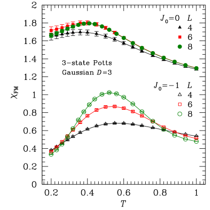
Figure 4: (Color online) Ferromagnetic susceptibility $\chi_{\rm FM}$ against $T$ for the three-state Potts glass with Gaussian couplings in three dimensions. The upper curves plotted with solid symbols correspond to $J_{0}=0$ while the lower curves with open symbols correspond to $J_{0}=-1$, where $J_{0}$ is the mean of the Gaussian interactions.

Table 2: Parameters of the simulation for the three-state Potts glass with Gaussian interactions in three dimensions used to compare results with $J_{0}=0$ and $J_{0}=-1$ where $J_{0}$ is the mean of the distribution. See Table 1 for details.

$L$	$J_{0}$	$T_{\mbox{\footnotesize min}}$	$N_{T}$	$N_{\mbox{\footnotesize samp}}$	$N_{\mbox{\footnotesize sw}}$
4	0	0.2	18	1000	81920
6	0	0.2	18	1000	81920
8	0	0.2	20	2400	655360
4	-1	0.2	18	1000	81920
6	-1	0.2	18	1000	81920
8	-1	0.2	20	2256	655360

As mentioned before, the Potts glass with $p>2$ develops ferromagnetic correlations at low temperatures even with $J_{0}=0$. To see the extent of this, we have performed additional simulations, with the parameters shown in Table 2, for $J_{0}=-1$ as well as $J_{0}=0$. We have calculated the ferromagnetic susceptibility, defined by

$$\chi_{\rm FM}=N[\langle\left|\mathbf{m}\right|^{2}\rangle]_{\mathrm{av}}\,,$$ (17)

where $\mathbf{m}=N^{-1}\sum_{i}\mathbf{S}_{i}$, and show the data in Fig. 4. For $J_{0}=0$, the ferromagnetic susceptibility grows slowly with temperature, seems to be bounded from above, and only displays a small system-size dependence. We therefore think that ferromagnetic correlations should not seriously affect the results presented earlier in this subsection. For $J_{0}=-1$, the absolute value of $\chi_{\rm FM}$ is smaller, but shows stronger size and temperature dependence. It seems that $\chi_{\rm FM}$ initially increases as $T$ is reduced, but then is strongly suppressed as spin-glass correlations develop for $T\to T_{\rm c}\simeq 0.27$. The spin-glass correlation length for both $J_{0}=0$ and $J_{0}=-1$ is shown in Fig. 5. The slope of the $J_{0}=-1$ data varies nonmonotonically with temperature, reflecting the nonmonotonic behavior of the ferromagnetic correlations. By contrast, the $J_{0}=0$ data vary much more smoothly. We further plot $\xi_{L}/L$ for $J_{0}=-1$ in Fig. 6. The observed nonmonotonic behavior of the slope suggests that corrections to finite-size scaling will be large and that the data in Fig. 2 should be more reliable in estimating $T_{\rm c}$. Nonetheless, the $J_{0}=-1$ data do have an intersection point, although at a lower temperature, $T\simeq 0.20$, than the value of $0.273$ for the $J_{0}=0$ case. We interpret these data to indicate that $T_{\rm c}\simeq 0.20$ for the $J_{0}=-1$ model (of course the value of $T_{\rm c}$ can vary with $J_{0}$). However, data on a larger range of sizes at lower temperature would be needed to confirm this. Unfortunately, equilibration times are very long at such low temperatures, so these calculations were not feasible.

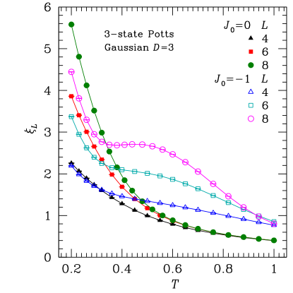
Figure 5: (Color online) Graph of $\xi_{L}$ vs $T$ for the three-state Potts glass with Gaussian couplings in three dimensions. The solid symbols correspond to $J_{0}=0$ while the open symbols correspond to $J_{0}=-1$.

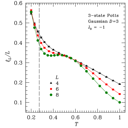
Figure 6: (Color online) Graph of $\xi_{L}/L$ vs $T$ for the three-state Potts glass with Gaussian couplings in three dimensions where the mean of the Gaussian distribution is $J_{0}=-1$. The vertical line is drawn at the transition temperature $T_{\rm c}=0.273$ of the $J_{0}=0$ case (see Fig. 2).

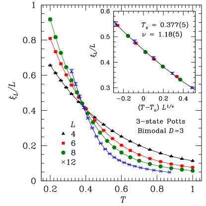
Figure 7: (Color online) Graph of $\xi_{L}/L$ vs $T$ for the three-state Potts glass with a bimodal coupling distribution in three dimensions. The curves intersect at $T_{\rm c}\simeq 0.377$. The inset shows a scaling plot according to Eq. (12) using $T_{\rm c}=0.377$ and $\nu=1.18$.

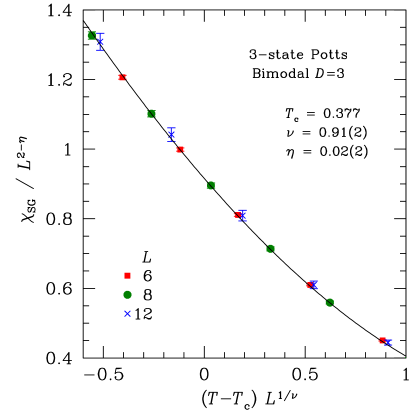
Figure 8: (Color online) Scaling plot of $\chi_{\rm SG}$ according to Eq. (13) with $T_{\rm c}$ fixed to 0.377 (determined from the data for $\xi_{L}/L$ shown in Fig. 7) for the three-state Potts glass with bimodal ($\pm J$) interactions in three dimensions. The fit to Eq. (13) then gives $\eta=0.02$ and $\nu=0.91$.

Table 3: Parameters of the simulation for the three-state Potts glass with bimodal interactions and $J_{0}=0$ in three dimensions. For further details see the caption of Table 1.

$L$	$T_{\mbox{\footnotesize min}}$	$N_{T}$	$N_{\mbox{\footnotesize samp}}$	$N_{\mbox{\footnotesize sw}}$
4	0.2	18	10000	5120
6	0.2	18	4971	40960
8	0.2	20	2046	1310720
12	0.320	20	550	4194304

III.2 Bimodal disorder ($\boldsymbol{d=3}$)

We expect that the value of the lower critical dimension and other universal quantities such as critical exponents are independent of the distribution of the interactions. To verify this we present in this subsection data for the three-state Potts glass in three dimensions with a bimodal ($\pm J$) distribution for comparison with the above results for the Gaussian distribution. The simulation parameters are shown in Table. 3.

Our results for $\xi_{L}/L$ are shown in Fig. 7. The data intersect at $T_{\rm c}\simeq 0.38$, indicating a spin-glass transition. Fitting the data for $\xi_{L}$ for $0.34<T<0.44$ and $L\geq 6$, we obtain

$$T_{\rm c}=0.377(5)\qquad\nu=1.18(5).$$ (18)

The scaling plot according to Eq. (12) is shown in the inset of Fig. 7.

Similar to the data with Gaussian disorder, the fits for $\chi_{\rm SG}$ give a different value for $T_{\rm c}$ from that obtained from data for $\xi_{L}/L$. Since we argue that the latter is more accurate, we have fitted $\chi_{\rm SG}$ with $T_{\rm c}$ fixed to the value $0.377$. This gives $\nu=0.91(2)$ and

$$\eta=0.02(2)\,.$$ (19)

These results are shown in Fig. 8.

If we allow $T_{\rm c}$ to fluctuate, the fits to the data for $\chi_{\rm SG}$ give $T_{\rm c}=0.390(21)$, $\nu=0.87(7)$, and $\eta=0.14(17)$. The error bars are larger than in the analysis when $T_{\rm c}$ is fixed, but the results are consistent with the previous analysis. Note that for the Gaussian case, $T_{\rm c}$ estimated from $\xi_{L}/L$ is greater than that from $\chi_{\rm SG}$, whereas it is lower for the $\pm J$ distribution. However, these differences are within the statistical errors and so are not significant. As discussed in Sec. III.3, the results from $\xi_{L}/L$ are expected to be more accurate than those from $\chi_{\rm SG}$. We can also analyze the $\chi_{\rm SG}$ data by fixing both $T_{\rm c}$ and $\nu$ to the values obtained from $\xi_{L}/L$ and so obtain just $\eta$. This gives $\eta=0.03(2)$ which is consistent with the result in Eq. (19).

Comparing our results in this subsection with those above for the Gaussian distribution, we see that in both cases we obtain a finite $T_{\rm c}$, showing that $d_{l}<3$. This is in contrast to the $T=0$ domain-wall renormalization group calculations of Banavar and CieplakBanavar and Cieplak (1989a, b) who find $d_{l}<3$ for the Gaussian distribution and $d_{l}>3$ for the $\pm J$ distribution. One possible reason for this difference is the larger range of sizes that we are able to treat in the present study.

Furthermore, the values for the exponent $\nu$ agree within the statistical errors and those for $\eta$ almost agree; see Eqs. (15), (16), (18), and (19). The small additional difference in the the values for $\eta$ can be attributed to systematic corrections to scaling. Hence our results are consistent with universality.

III.3 Gaussian disorder ($\boldsymbol{d=4}$)

Table 4: Parameters of the simulation for the three-state Potts glass with Gaussian interactions and $J_{0}=0$ in four dimensions. For further details see the caption of Table 1.

$L$	$T_{\mbox{\footnotesize min}}$	$N_{T}$	$N_{\mbox{\footnotesize samp}}$	$N_{\mbox{\footnotesize sw}}$
3	0.2	18	1044	40960
4	0.2	18	2691	40960
5	0.350	17	1000	524288
6	0.408	18	700	327680
8	0.490	22	623	524288

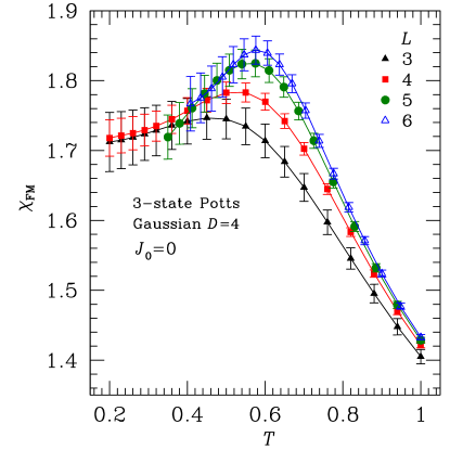
Figure 9: (Color online) Graph of $\chi_{\rm FM}$ vs $T$ for the three-state Potts glass with Gaussian couplings with $J_{0}=0$ in four dimensions.

For the three-state Potts glass in four dimensions we first show data for $\chi_{\rm FM}$ with $J_{0}=0$ in Fig. 9 to see whether significant ferromagnetic correlations develop. The behavior is very similar to the case in $d=3$ (see Fig. 4) since $\chi_{\rm FM}$ remains small and relatively size independent. This indicates that ferromagnetic couplings, while present, are relatively weak thus we set $J_{0}=0$ in the simulations of the three-state model in $d=4$. The simulation parameters are presented in Table 4.

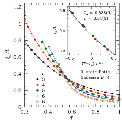
Figure 10: (Color online) Correlation length $\xi_{L}/L$ vs $T$ for the three-state Potts glass with Gaussian couplings in four dimensions. The curves intersect at $T_{\rm c}\simeq 0.54$. The inset shows a scaling plot according to Eq. (12) using $T_{\rm c}=0.536$ and $\nu=0.81$.

Next we plot $\xi_{L}/L$ in Fig. 10, where the data intersect at $T_{\rm c}\approx 0.54$. Fitting the data for $\xi_{L}$ for $0.49<T<0.59$ and $L\geq 4$, we obtain the best fit as

$$T_{\rm c}=0.536(3),\qquad\nu=0.81(2)\,.$$ (20)

The scaling plot according to Eq. (12) is shown in the inset of Fig. 10.

Our value for $T_{\rm c}$ is very different from that of Scheucher and RegerScheucher and Reger (1993) who estimate $T_{\rm c}=0.25(5)$. However, in the vicinity of their estimate for $T_{\rm c}$ they could equilibrate only two small sizes $L=3$ and 4. Furthermore, they used the Binder ratioBinder (1981) (a ratio of moments of the order parameter) which even fails to intersectDillmann et al. (1998) at the known transition temperature in the mean-field Potts model. Hence we feel that our approach, using the correlation length, is more reliable, especially since we are able to use parallel tempering to simulate larger sizes at lower $T$ than was possible for Scheucher and Reger in the “pre-parallel tempering days.”

We next discuss the data for $\chi_{\rm SG}$. First we fix $T_{\rm c}$ to be the value 0.536 obtained from $\xi_{L}/L$. Fitting to Eq. (13) then gives $\nu=0.70(1)$ and

$$\eta=-0.08(2).$$ (21)

This is shown in Fig. 11. We can also analyze the $\chi_{\rm SG}$ data by fixing both $T_{\rm c}$ and $\nu$ to the values obtained from $\xi_{L}/L$, and so obtain just $\eta$. This gives $\eta=-0.08(2)$ which agrees with the result in Eq. (21).

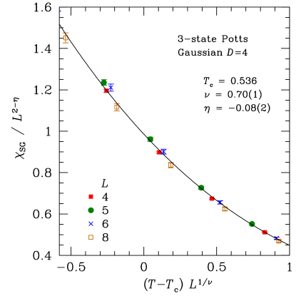
Figure 11: (Color online) Scaling plot of $\chi_{\rm SG}$ for the three-state Potts glass with Gaussian interactions in four dimensions according to Eq. (13) with $T_{\rm c}$ fixed to the value $0.536$, which is obtained from the data for $\xi_{L}/L$ shown in Fig. 10. The fit to Eq. (13) then gives $\eta=-0.08$ and $\nu=0.70$.

However, if we allow $T_{\rm c}$ to vary, as well as $\nu$ and $\eta$, we obtain $T_{\rm c}=0.505(14)$, $\nu=0.75(3)$, and $\eta=-0.46(16)$. We see that $T_{\rm c}$ is substantially lower than in Eq. (20). The resulting value of $\nu$ is not very different than that obtained in Eq. (20) but the value of $\eta$ is significantly more negative than that obtained in Eq. (21). These differences are due to corrections to finite-size scaling. A related problem of different exponents from $\chi_{\rm SG}$ and $\xi_{L}/L$ was also foundKatzgraber et al. (2006) for the Ising spin glass (although there the main discrepancy involved $\nu$ rather than $\eta$). They argued that the data for $\xi_{L}/L$ is the most accurate way to determine $T_{\rm c}$ and $\nu$. Since it is dimensionless, the data give clean intersections without having to divide by an unknown power of $L$. Reference Katzgraber et al., 2006 confirmed this supposition by reanalyzing their data in an alternative way proposed in Ref. Campbell et al., 2006. The results from $\xi_{L}/L$ did not change significantly, but the value for $\nu$ from $\chi_{\rm SG}$ changed considerably and became much closer to the value found from $\xi_{L}/L$.

Hence, for the present case, we feel that the values of $\nu$ in Eq. (20) (obtained from $\xi_{L}/L$) and $\eta$ in Eq. (21) (obtained from $\chi_{\rm SG}$ with $T_{\rm c}$ fixed at the value from $\xi_{L}/L$) are the most accurate ones. An estimate for the order parameter exponent $\beta$ is then obtained from the scaling relation

$$\beta=(d-2+\eta)\,\frac{\nu}{2}\,,$$ (22)

which gives

$$\beta=0.78(3)\,.$$ (23)

This is very different from the value $\beta\simeq 0$ obtained by Scheucher and Reger.Scheucher and Reger (1993) Therefore, we find that the transition in the three-state Potts glass in four dimensions is actually not in the mean-field universality classGross et al. (1985) for $p>4$.

IV Ten-state Potts glass in $\boldsymbol{d=3}$ (Gaussian disorder)

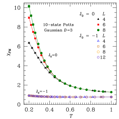
Figure 12: (Color online) Ferromagnetic susceptibility $\chi_{\rm FM}$ vs $T$ for the ten-state Potts glass with Gaussian couplings in three dimensions. For $J_{0}=-1$, represented by the open symbols, $\chi_{\rm FM}$ remains small and size independent. In contrast, $\chi_{\rm FM}$ for $J_{0}=0$ (solid symbols) becomes very large and shows substantial finite-size effects.

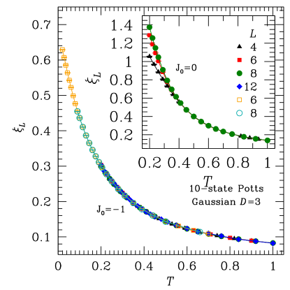
Figure 13: (Color online) Correlation length $\xi_{L}$ (not $\xi_{L}/L$) against $T$ for the ten-state Potts glass in three dimensions. The main panel shows the case for $J_{0}=-1$ where there are hardly any finite-size effects. The inset shows the same for $J_{0}=0$ showing the size dependence of $\xi_{L}$ in this case.

Finally, we turn our attention to the ten-state Potts glass in three dimensions with Gaussian interactions. We set the mean of the Gaussian interactions to $J_{0}=-1$ in order to suppress ferromagnetic ordering.Brangian et al. (2003) The effectiveness of this is shown in Fig. 12, where the ferromagnetic susceptibility $\chi_{\rm FM}$ is seen to be very small and does not exhibit measurable finite-size effects. However, if we take $J_{0}=0$, which is also shown, $\chi_{\rm FM}$ becomes large and size dependent, indicating that ferromagnetic ordering probably takes place. The simulation parameters used for the ten-state Potts glass for $J_{0}=-1$ are shown in Table 5. The second set of parameters for $L=6$ and $8$ is for additional runs to probe the very-low-temperature behavior.

A plot of $\xi_{L}$ (not divided by $L$) against temperature for $J_{0}=-1$ is shown in Fig. 13. The correlation length shows no size dependence and stays very small, less than one lattice spacing, even at extremely low temperatures. We conclude, in agreement with Brangian et al.,Brangian et al. (2003) that there is clearly no spin-glass transition in this model.

Table 5: Parameters of the simulation for the ten-state Potts glass with Gaussian interactions with $J_{0}=-1$ in three dimensions. The second set of parameters for $L=6$ and $8$ is for additional runs to probe the very low-temperature behavior of the model.

$L$	$T_{\mbox{\footnotesize min}}$	$N_{T}$	$N_{\mbox{\footnotesize samp}}$	$N_{\mbox{\footnotesize sw}}$
4	0.2	14	1000	81920
6	0.2	17	1000	131072
8	0.2	19	998	262144
12	0.2	26	343	20480
6	0.02	28	469	262144
8	0.08	18	600	131072

Since the nearest-neighbor ten-state Potts glass does not even come close to having a transition down to $T=0$, its behavior is very different from the mean-field (infinite-range) case, which has two transitions. Although the mean-field version provides a plausible model for supercooled liquids as they are cooled down towards the glass transition, the nearest-neighbor model does not. It might therefore be interesting to investigate a Potts glass that has somewhat longer-range interactionsBrangian et al. (2003) to see if its behavior corresponds more closely to that of supercooled liquids.

V Conclusions

Table 6: Summary of results for the four different $p$-state Potts glasses studied. The values for $T_{\rm c}$ and $\nu$ are obtained from analyzing data for $\xi_{L}/L$, which we argue give the most reliable results. The values for $\eta$ are obtained from data for $\chi_{\rm SG}$ with only $T_{\rm c}$ fixed to its value obtained from $\xi_{L}$.

$p$	Disorder	$d$	$T_{\rm c}$	$\nu$	$\eta$
3	Gaussian	3	$0.273(5)$	$1.30(7)$	$-0.03(2)$
3	Bimodal ($\pm J)$	3	$0.377(5)$	$1.18(5)$	$0.02(2)$
3	Gaussian	4	$0.536(3)$	$0.81(2)$	$-0.08(2)$
10	Gaussian	3	No transition

We show a summary of our results for the various models in Table. 6. We find strong evidence for a finite transition temperature $T_{\rm c}$ in the three-state Potts glass in three dimensions, with universal critical exponents. This differs from several earlier studies which claimed that the lower critical dimension is equal or close to $3$. In four dimensions, the three-state Potts glass has a transition which is quite different from that proposed by Scheucher and RegerScheucher and Reger (1993)—namely the discontinuous transition found in mean-field theory for $p>4$. The ten-state Potts glass in three dimensions, which in its mean-field incarnation is often used to describe structural glasses, is very far from having a phase transition into a glassy phase at any temperature since its correlation length remains very small even down to extremely low temperatures, in agreement with the work of Brangian et al.Brangian et al. (2003)