Magnetosubband and edge state structure in cleaved-edge overgrown quantum wires

Abstract

We provide a systematic quantitative description of the structure of edge states and magnetosubband evolution in hard wall quantum wires in the integer quantum Hall regime. Our calculations are based on the self-consistent Green’s function technique where the electron- and spin interactions are included within the density functional theory in the local spin density approximation. We analyze the evolution of the magnetosubband structure as magnetic field varies and show that it exhibits different features as compared to the case of a smooth confinement. In particularly, in the hard-wall wire a deep and narrow triangular potential well (of the width of magnetic length $l_{B}$) is formed in the vicinity of the wire boundary. The wave functions are strongly localized in this well which leads to the increase of the electron density near the edges. Because of the presence of this well, the subbands start to depopulate from the central region of the wire and remain pinned in the well region until they are eventually pushed up by increasing magnetic field. We also demonstrate that the spin polarization of electron density as a function of magnetic field shows a pronounced double-loop pattern that can be related to the successive depopulation of the magnetosubbands. In contrast to the case of a smooth confinement, in hard-wall wires the compressible strips do not form in the vicinity of wire boundaries and spatial spin separation between spin-up and spin-down states near edges is absent.

I Introduction

Recent advances in fabrication of low-dimensional structures allow one to create quantum wires with a hard-wall potential confinement. The available technologies include implantation-enhanced interdiffusion technique Cibert developed more than 20 years ago. Using this technique Prins et al. Prins demonstrated a potential jump at a hetero-interface GaAs-AlGaAs over only 8 nm distance. The molecular beam epitaxy double-growth technique Pfeiffer1 (often referred to as a cleaved-edge overgrowth) since early 1990-th has become one of the most widely-used techniques for fabrication of quantum wires Yacoby ; Yacoby2 ; Motoshita and two-dimensional electron gases (2DEGs) Huber with an essentially hard wall confinement with the atomic precision. Quantum wires with a steep confinement can also be fabricated by overgrowth on patterned GaAs(001) substrates using molecular beam epitaxy Shitara .

For theoretical description of the quantum Hall effect in quantum wires, a concept of edge states is widely usedHalperin . In a naive one-electron picture a position of the edge states are determined by the intersection of the Landau levels (bent by the bare potential) with the Fermi energy, and their width is given by a spatial extension of the wave function, which is of the order of the magnetic length $l_{B}=\sqrt{\frac{\hbar}{eB}}$. For a smooth electrostatic confinement that varies monotonically throughout the cross-section of a wire, Chklovskii at al.Chklovskii have shown that electrostatic screening in strongly modifies the structure of the edge states giving rise to interchanging compressible and incompressible strips. The electrons populating the compressible strips screen the electric field, which leads to a metallic behavior when the electron density is redistributed (compressed) to keep the potential constant. The neighboring compressible strips are separated from each other by insulator-like incompressible strips corresponding to the fully filed Landau levels with a constant electron density.

A number of studies of quantum wires with a smooth confinement have been reported during the recent decadeKinaret ; Ando_1993 ; Dempsey ; Tejedor ; Gerhardts_1994 ; Tokura ; Stoof ; Ferconi_1995 ; Takis ; Ando_1998 ; Schmerek ; Gerhardts_2004 addressing the problem of electron-electron interaction beyond Chklovskii at al.’sChklovskii electrostatic treatment. A particular attention has been paid to spin polarization effects in the edge states Kinaret ; Dempsey ; Tokura ; Takis ; Stoof ; Ihnatsenka ; Ihnatsenka2 . It has been demonstrated that the exchange and correlation interactions dramatically affect the edge state structure in quantum wires bringing about qualitatively new features in comparison to a widely used model of spinless electrons. These include spatial spin polarization of the edge statesDempsey ; Ihnatsenka2 , pronounced $1/B$-periodic spin polarization of the electron densityIhnatsenka , modification and even suppression of the compressible stripsIhnatsenka2 and others. It should be stressed that all the above-mentioned studies addressed the case of a soft confinement corresponding to e.g. a gate-induced depletion when the Borh radius is much smaller that the depletion length. In fact, Huber et al. have recently presented experimental evidence that widely used concept of compressible/incompressible stripsChklovskii does not apply to the case of a sharp-edge 2DEG. At the same time the rigorous theory for edge-state structure in hard-wall quantum wires accounting for electron-electron interaction and spin effects has not been reported yet. Such a theory is obviously required for a detailed analysis of recent experiments on cleaved-edge overgrown sharp-edge wires and 2DEGs Prins ; Pfeiffer1 ; Huber ; Yacoby ; Yacoby2 ; Motoshita ; Shitara .

Motivated by the above-mentioned experimental studies, in this paper we present a detailed theory of magnetosubband and edge state structure in quantum wires with a hard wall confinement taking into account electron-electron interaction including exchange and interaction effects. We employ an efficient numerical tool based on the Green’s function technique for self-consistent solution of the Schrödinger equation in the framework of the density functional theory (DFT) in the local spin density approximation (LSDA)ParrYang . The choice of DFT+LSDA for description of many-electron effects is motivated, on one hand, by its efficiency in practical implementation within a standard Kohn-Sham formalism Kohn , and, on the other hand, by an excellent agreement between the DFT+LSDA and the exact diagonalization Ferconi and the variational Monte-Carlo calculationsRasanen ; QDOverview performed for few-electron quantum dots. We will demonstrate below that edge state structure of the hard wall quantum wire is qualitatively different from that of the soft-wall wire. We will discuss how the spin-resolved subband structure, the current densities, the confining potentials, as well as the spin polarization in the hard wall quantum wire evolve when an applied magnetic field varies.

The paper is organized as follow. In Sec. II we present a formulation of the problem, where we define the geometry of the system at hand and outline the self-consistent Kohn-Sham scheme within the DFT+LSDA approximation. In Sec. III we present our results for a hard wall quantum wire calculated within Hartree and DFT+LSDA approximations, where we distinguish cases of wide and narrow wires. Section IV contains our conclusions.

II Model

We consider a quantum wire which is infinitely long in the $x$-direction and is confined by a hard-wall potential in the $y$-direction, see Fig. 1.

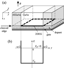
Figure 1: (Color online). (a) A schematic illustration of a cleaved-edge overgrown quantum wire and (b) a corresponding hard-wall confinement potential.

The magnetic field is applied perpendicular to the $xy$-plane. We set the Fermi energy $E_{F}=0$. A bottom of the confining potential is flat and situated at $E=V_{0}$. We limit ourself to a typical case when only one subband is occupied in the transverse $z$-directionHuber such that electron motion is confined to the $xy$-plane. The Hamiltonian of the wire reads $H=\sum_{\sigma}H^{\sigma}$,

$$H^{\sigma}=H_{0}+V_{0}+V_{eff}^{\sigma}(y)+g\mu_{b}B\sigma,$$ (1)

where $H_{0}$ is the kinetic energy in the Landau gauge,

$$H_{0}=-\frac{\hbar^{2}}{2m^{\ast}}\left\{\left(\frac{\partial}{\partial x}-\frac{eiBy}{\hbar}\right)^{2}+\frac{\partial^{2}}{\partial y^{2}}\right\},$$ (2)

where $\sigma=\pm\frac{1}{2}$ describes spin-up and spin-down states, $\uparrow$, $\downarrow$, and $m^{\ast}=0.067m_{e}$ is the GaAs effective mass. The last term in Eq. (1) accounts for Zeeman energy where $\mu_{b}=\frac{e\hbar}{2m_{e}}$ is the Bohr magneton, and the bulk $g$ factor of GaAs is $g=-0.44$. The effective potential, $V_{eff}(y)$ within the framework of the Kohn-Sham density functional theory reads Kohn ,

$$V_{eff}^{\sigma}(y)=V_{H}(y)+V_{ex}^{\sigma}(y),$$ (3)

where $V_{H}(y)$ is the Hartree potential due to the electron density $n(y)=\sum_{\sigma}n^{\sigma}(y)$ (including the mirror charges) Ihnatsenka ,

$$V_{H}(y)=-\frac{e^{2}}{4\pi\varepsilon_{0}\varepsilon_{r}}\int dy^{\prime}n(y^{\prime})\ln\frac{\left(y-y^{\prime}\right)^{2}}{\left(y-y^{\prime}\right)^{2}+4b^{2}}.$$ (4)

with $2b$ being the distance from the electron gas to the mirror charges (we choose $b$=60 nm). For the exchange and correlation potential $V_{xc}(y)$ we utilize the widely used parameterization of Tanatar and Cerperly TC (see Ref. Ihnatsenka, for explicit expressions for $V_{xc}(y)$). This parameterization is valid for magnetic fields corresponding to the filling factor $\nu>1$, which sets the limit of applicability of our results. The spin-resolved electron density reads

$$n^{\sigma}(y)=-\frac{1}{\pi}\Im\int dE\,G^{\sigma}(y,y,E)f_{FD}(E-E_{F}),$$ (5)

where $G^{\sigma}(y,y,E)$ is the retarded Green’s function corresponding to the Hamiltonian (1) and $f_{FD}(E-E_{F})$ is the Fermi-Dirac distribution function. The Green’s function of the wire, the electron and current densities are calculated self-consistently using the technique described in detail in Ref. Ihnatsenka, .

The current density for a mode $\alpha$ is calculated as Ihnatsenka

$$J_{\alpha}^{\sigma}(y)=\frac{e^{2}}{h}V\int dE\frac{j_{\alpha}^{\sigma}(y,E)}{v_{\alpha}^{\sigma}}\left(-\frac{\partial f\left(E-E_{F}\right)}{\partial E}\right),$$ (6)

with $v_{\alpha}^{\sigma}$ and $j_{\alpha}^{\sigma}(y,E)$ being respectively the group velocity and the quantum-mechanical particle current density for the state $\alpha$ at the energy $E$, and $V$ being the applied voltage.

We also calculate a thermodynamical density of states ($TDOS$) defined according to Davies ; Manolescu

$$TDOS^{\sigma}=\int dE\,\rho^{\sigma}(E)\left(-\frac{\partial f_{FD}(E-E_{F})}{\partial E}\right),$$ (7)

where the spin-resolved density of states $\rho^{\sigma}(E)$ is given by the Green functionDatta ,

$$\rho^{\sigma}(E)=-\frac{1}{\pi}\Im\int dy\,\,G^{\sigma}(y,y,E).$$ (8)

The $TDOS$ reflects a structure of the magnetosubbands near the Fermi energy and it can be accessible via magneto-capacitance Weiss or magnetoresistance Berggren measurements. Indeed, a compressible strip corresponds to a flat (dispersionless) subband pinned at $E_{F}$. In this case $\rho^{\sigma}(E)$ is high at $E\approx E_{F}$ and such the subband strongly contributes to $TDOS$. In contrast, in an incompressible strip, subbands are far away from $E_{F}$ and do not contribute to $TDOS$. Thus $TDOS$ is proportional to the area of the compressible strips. This area is maximal when the strip if formed in the middle of a quantum wire. In this case the backscattering between opposite propagating states is maximal, which corresponds to peaks in the longitudinal resistance $R_{xx}$ (seen as the Shubnikov-De Haas oscillations) Berggren ; Hwang ; Beenakker . In magneto-capacitance experimentsWeiss ; Beenakker the compressible strips are viewed as capacitor plates and therefore the measured magnetocapacitance is related to the width of these strips. Thus the peaks in the $TDOS$ are manifest themselves in both $R_{xx}$ and capacitance peaks.

III Results and discussion

In what follows we shall distinguish between cases of a wide quantum wire whose half-width $\frac{w}{2}$ exceeds the magnetic length $l_{B},$ and a narrow wire with a width $\frac{w}{2}\lesssim$ $l_{B}.$

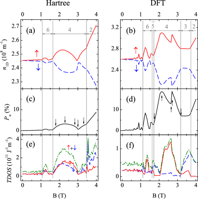
Figure 2: (Color online). (a),(b) One-dimensional charge density for the spin-up and spin-down electrons, $n_{1D}^{\uparrow},\ n_{1D}^{\downarrow}$; (c),(d) the spin polarization of the charge density, $P_{n}=\frac{n_{1D}^{\uparrow}-n_{1D}^{\downarrow}}{n_{1D}^{\uparrow}+n_{1D}^{\downarrow}}$, (g),(h) the $TDOS$ for spin-up and spin-down electrons and the total $TDOS$ within the Hartree approximation and the DFT approximation (first and second columns, respectively). The number of subband is indicated in (a),(b). Arrows in (c) and (d) indicate the magnetic field corresponding to the magnetosubband structure shown in Figs. 3 and 4. The width of the wire is $w=300$ nm and the depth is $V_{0}=-0.1$ eV. Temperature $T=1$ K.

III.1 Wide hard wall quantum wire $\frac{w}{2}>l_{B}$

Let us consider a hard wall quantum wire of the width $w=300$ and $V_{0}=-0.1$ eV. With these parameters the wire has $N\sim 20$ spin-resolved occupied subbands at zero magnetic field, and the sheet electron density in its center is $n_{2D}\approx 1.5\cdot 10^{15}$ m^-2 (as calculated self-consistently in both Hartree and DFT approximations).

Hartree approximation

We start our analysis of the edge state- and magnetosubband structure from the case of the Hartree approximation (when the exchange and correlation interactions are not included in the effective potential). The Hartree approximation gives the structure of the compressible/incompressible strips which serves as a basis for understanding of the effect of the exchange and correlation within the DFT approximationIhnatsenka ; Ihnatsenka2 .

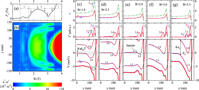
Figure 3: (Color online). (a) Spin polarization of the charge density as a function of $B$ calculated within the Hartree approximation (the same as Fig. 2(c)). (b) Spatially resolved difference in the electron density $n^{\uparrow}(y)-n^{\downarrow}(y)$. (c)-(g) The subband structure for magnetic fields indicated by arrows in (a). Upper panel: electron density profiles (local filling factors) $\nu(y)=n(y)/n_{B}$ for spin-up and spin-down electrons; middle panel: the current density distribution for spin-up and spin-down electrons; lower panel: magnetosubband structure for spin-up and spin-down electrons. Fat solid and dashed lines indicate the total confining potential for respectively spin-up and spin-down electrons. The width of the wire is $a=300$ nm and depth is $V_{0}=-0.1$ eV. Temperature $T$=1 K.

Figure 2(a) shows the 1D electron density $n_{1D}^{\sigma}=\int n^{\sigma}(y)dy$ for the spin-up and spin-down electrons in the quantum wire. The pronounced feature of this dependence is a characteristic loop pattern of the charge density polarization, $P_{n}=\frac{n_{1D}^{\uparrow}-n_{1D}^{\downarrow}}{n_{1D}^{\uparrow}+n_{1D}^{\downarrow}}$, see Fig. 2(b) . Figure 2 also indicates a number of magnetosubbands $N$ populated at a given $B$. The number of subbands is always even such that spin-up and spin-down subbands depopulate practically simultaneously. This is because the spin polarization within the Hartree approximation is driven by Zeeman splitting only, which is small in the field interval under consideration. A comparison of Figs. 2(a),(c),(e) demonstrates that the spin polarization as well as the $TDOS$ are directly related to the magnetosubband structure. Note that a similar loop-like behavior of the spin polarization is also characteristic for a split-gate wire with a smooth confinementIhnatsenka . For the latter case the polarization calculated in the Hartree approximation drops practically to zero when the subbands depopulate (see Fig. 4 in Ref. Ihnatsenka, ). In contrast, in the case of the hard wall confinement, the polarization loops exhibit more complicated pattern: the polarization does not drop to zero when the subbands depopulate, and, in addition, the polarization curves show a double loop-like pattern with an additional minimum (e.g. at $B\approx 1.5$T, 3T in Fig. 2 (a),(c)). In order to understand the origin of this behaviour let us analyze the evolution of the subband structure as the applied magnetic field varies. Let us concentrate at the field interval 1.65 T $\lesssim B\lesssim$ 3.5 T when the subband number $N=4$.

Figure 3(b) shows the spatially resolved difference in the electron density $n^{\uparrow}(y)-n^{\downarrow}(y)$ as a function of $B$. The electron density is mostly polarized in the inner region of the quantum wire. For certain ranges of magnetic fields the electron density shows a strong polarization in the boundary regions, which are separated from the polarized inner region by wide unpolarized strips (e.g. for $3\text{T}\lesssim B\lesssim 3.5\text{T}$). We will show below that this feature reflects the peculiarities of the magnetosubband structure for the case of the hard wall confinement. Figure 3(c) shows the electron density profiles (local filling factors) $\nu(y)=n(y)/n_{B}$ $(n_{B}=eB/h)$, the current densities $J^{\sigma}(y)$ and the magnetosubband structure for the magnetic field $B=1.8$ T. At this field a wide compressible strip due to electrons belonging to the subbands $N=3,4$ is formed in the middle of the wire. (Following Suzuki and AndoAndo_1998 we define the width of the compressible strips within the energy window $|E-E_{F}|<2\pi kT$ corresponding to the partial occupation of the subbands when $f_{FD}<1$; this energy window is indicated in Fig. 3 (c)). Partial subband occupation combined with Zeeman splitting of energy levels results in different population for spin-up and spin-down electrons (i.e. in the spin polarization of the electron density).

Close to the wire edges the total potential exhibits a narrow and deep triangular well. The formation of the triangular well is also reflected in the structure of the magnetosubbands that show triangular wells near the wire edges. Presence of these triangular wells is a distinctive feature of the hard-wall confinement (it is absent for the case of a smooth confinement in the split-gate wiresAndo_1993 ; Ando_1998 ; Ihnatsenka ; Ihnatsenka2 ). The wave functions for all subbands are strongly localized in these wells, with the extension of the wave functions being of the order of the magnetic length $l_{B}$. Because of steepness of the potential walls, the wave functions are not able to screen the confining potential, and compressible strips can not form near the wire boundary. This is in a stark contrast to the case of a split-gate wire where the compressible strips near edges are formed for a sufficiently smooth confinementChklovskii ; Ando_1998 ; Ihnatsenka ; Ihnatsenka2 . The electron density near the wire boundaries does not show any spin polarization. This is because the bottom of the potential well lies far below the Fermi energy. As a result, both spin-up and spin-down states localized in the quantum well are completely filled ($f_{FD}=1$) and the spin polarization is absent.

When a magnetic field increases the compressible strip in the middle of the wire widens. This is accompanied by increase of both the spin polarization and the $TDOS$ as shown in Figs. 2(c),(e). At $B=2.3$T the polarization reaches maximum $P_{n}=3$ % which corresponds to the maximum width of the compressible strip in the central part of the wire, see Fig. 3(d). With further increase of the magnetic field 3rd and 4th subbands in the central part of the wire are pushed up, see Fig. 3(e). Their population decreases according to the Fermi-Dirac distribution and, consequently, the spin polarization diminishes. At the same time, fully occupied parts of 3rd and 4th subbands (forming a triangular well near the wire boundaries) are pushed up and got pinned at the Fermi energy. This is accompanied by a formation of a potential barrier at the distance of the wave function extent $\sim l_{B}$ from the wire edges, see Fig. 3(e). The whole area occupied by subbands 3 and 4 becomes divided by non-populated region within the barrier where the subbands lie above $E_{F}$ (i. e. $f_{FD}=0$).

When a magnetic field slightly increases from $B=2.8$T to $B=3.0$T the magnetosubband structure undergoes significant changes. A middle part of the 3rd and 4th subbands is abruptly pushed up in energy. The incompressible strip emerges here due to 1st and 2nd fully occupied subband lying well below $E_{F}$, Fig. 3(f). As a result the spin polarization decreases and the fist polarization loop closes down at $B\approx 3$T, see 3(a). Note that $P_{n}$ does not drop to zero because of a finite polarization at the boundaries where the 3rd and 4th subband bottoms are still pinned at the Fermi energy, see Fig. 3(b),(f). As magnetic field increases the second polarization loop starts to form at $B\approx 3$T due to 1st and 2nd subbands that get pinned to $E_{F}$ in the middle of the wire (Fig. 3(g)). In addition, 3rd and 4th subbands that are pinned to $E_{F}$ near the wire boundaries also contribute to spin polarization. These subbands become completely depopulated at $B=3.5$ T. Further increase of the magnetic field causes the compressible strip in the middle to widen. The spin polarization $P_{n}$ grows linearly until the second subband becomes depopulated.

Note that the above scenario of the subband depopulation in quantum wires with a hard wall confinement is qualitatively different from that one of the smooth confinement. In the former case, because of the presence of the deep triangular well near the wire boundaries, the subbands start to depopulate from the central region of the wire and remain pinned in the well region until they are eventually pushed up by magnetic field. In contrast, in the case of a smooth confinement, the subband always depopulate from the edges, such that a compressible strip in the middle of the wire gradually decreases until it completely disappears when the whole subband is pushed up above the Fermi energyIhnatsenka ; Ihnatsenka2 .

The spatial current distribution stays practically the same throughout the magnetosubband evolution, see the central panel in Figs. 3(c)-(g). This is due to a strong localization of electrons in the triangular potential well. The spatial spin separation between spin-up and spin-down states is always equal to zero, which is also the case for a split-gate wire in the Hartree approximation Ihnatsenka ; Ihnatsenka2 .

Finally, within the Hartree approximation the $TDOS$ shows a behavior similar to the spin polarization of the electron density $P_{n}$, compare Fig. 2(e) and 2(c). This is because the spin polarization is primarily caused by electrons in the compressible strips, and the $TDOS,$ as discussed in the previous section, is proportional to the width of these strips.

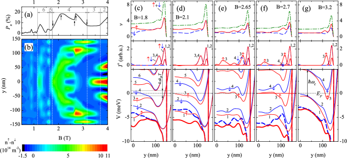
Figure 4: (Color online). (a) Spin polarization of the charge density as a function of $B$ calculated within the DFT approximation (similar to Fig. 2(d)). (b) Spatially resolved difference in the electron density $n^{\uparrow}(y)-n^{\downarrow}(y)$. (c)-(g) The subband structure for magnetic fields indicated by arrows in (a). Upper panel: electron density profiles (local filling factors) $\nu(y)=n(y)/n_{B}$ for spin-up and spin-down electrons; middle panel: the current density distribution for spin-up and spin-down electrons; lower panel: magnetosubband structure for spin-up and spin-down electrons. Fat solid and dashed lines indicate the total confining potential for respectively spin-up and spin-down electrons. The width of the wire is $a=300$ nm and depth is $V_{0}=-0.1$ eV. Temperature $T=1$K.

DFT approximation

The exchange and correlation interactions bring qualitatively new features to the magnetosubband structure in comparison to the Hartree approximation. Figures 2(b),(d),(f) show the 1D electron density, the number of subbands, the spin polarization and the $TDOS$ calculated within DFT approximation. There are several major differences in comparison to the Hartree case. First, the spin polarization of the electron density also shows a pronounced loop pattern. However, for a given magnetic field the spin polarization in the quantum wire calculated on the basis of the DFT approximation is much higher in comparison to the Hartree approximation (by a factor 5-10). Second, the exchange interaction lifts subband degeneration, such that the subbands depopulate one by one. Third, the $TDOS$ reveals peaks which are attributed to different spin species.

Before we proceed to analysis of the magnetosubband structure within the DFT approximation, it is instrumental to outline the effect of the exchange interaction on the subband spin splitting. Within the Hartree approximation the subbands are practicably degenerate because the Zeeman splitting is very small in the magnetic field interval under investigation. In contrast, the exchange interaction included within the DFT approximation causes the separation of the subbands which magnitude can be comparable to the Landau level spacing $\hbar\omega$. Indeed, the exchange potential for spin-up electrons depends on the density of spin-down electrons and vice versaParrYang ; TC ; Ihnatsenka . In the compressible region the subbands are only partially filled (because $f_{FD}<1$ in the the window $|E-E_{F}|\lesssim 2\pi kT$), and, therefore, the population of the spin-up and spin-down subbands can be different. In the DFT calculation, this population difference (triggered by Zeeman splitting) is strongly enhanced by the exchange interaction leading to different effective potentials for spin-up and spin-down electrons and eventually to the subband spin splitting. Below the Fermi energy $E\lesssim E_{F}-2\pi kT$ the subbands remain degenerate because they are fully occupied ($f_{FD}=1$). As a result, the corresponding spin-up and spin-down densities are the same, hence the exchange and correlation potentials for the spin-up and spin-down electrons are equal, $V_{xc}^{\uparrow}(y)=V_{xc}^{\downarrow}(y)$.

In order to understand the effect of the exchange-correlation interactions on evolution of the magnetosubband structure, let us concentrate on the same field interval as discussed in the case of the Hartree approximation, 1.8 T $\lesssim B\lesssim$ 3.7 T. A comparison between Fig. 4 and Fig. 3 demonstrates that evolution of the magnetosubband structure calculated within the DFT approximation follows the same general pattern as for the case of the Hartree approximation. In particularly, a deep triangular well near the wire boundary develops in the total confining potential for both spin-up and spin-down electrons. The wave functions are strongly localized in this well. As a result, similarly to the Hartree case, the depopulation of the subbands starts from the central region of the wire. The subbands remain pinned in the well region until they are eventually pushed up by magnetic field. The major difference from the Hartree case is that Hartree subbands are practically degenerated and depopulate together, whereas this degeneracy is lifted by the exchange interaction such that DFT subbands depopulate one by one. Indeed, Figs. 4 (c),(d) showing consecutive depopulation of the subbands 4 and 3 in the central region of the wire can be compared with the corresponding evolution of the Hartree subbands in Figs. 3 (c),(d). When the magnetic field increases further, 3rd subband bends upward in the vicinity of the triangular well, compare Fig. 4 (e) and Fig. 3 (e). When magnetic field reaches $B\approx 2.7$T, 4th spin-down subband becomes completely depopulated and 3rd spin-up subband is occupied mostly in the region of the triangular well near the wire boundary, see Fig. 3 (f). This leads to a strong spin polarization near the boundary which is manifest itself in the additional loop of the polarization (see Fig. 2 (b), 2.7T$\lesssim B\lesssim$3.2T). Note that this loop is absent in the Hartree calculations because both 3rd and 4th subbands are occupied in the well region, such that the spin splitting between them is small (see Fig. 3 (f)). Finally, 3rd subband becomes fully depopulated in the central region, and a compressible strip starts to form there due to 2nd subband that is pushed upwards, compare Figs. 4 (g) and Fig. 3 (g).

Note that similarly to the case of the Hartree approximation, the evolution of the magnetosubband structure within the DFT approximation described above qualitatively holds for all other polarization loops.

We also stress that in contrast to the case of a smooth confinementIhnatsenka ; Ihnatsenka2 , in hard-wall wires the compressible strips do not form in the vicinity of wire boundaries and a spatial spin separation between spin-up and spin-down states near edges is absent.

Oscillations of the $TDOS$ calculated within the DFT approximation shows that neighboring peaks belong to different spin species (Fig. 2(f)). In contrast, the Hartree approximation shows that each single peak includes equal contributions from both species (Fig. 2(e)). It is interesting to note that the oscillation of the $TDOS$ do not exactly correspond to the subband depopulation. Instead, they reflect formation of the compressible strip in the middle of the wire due to spin-up and spin-down electrons which is not directly related to the subband depopulation (which takes place in the region of the triangular well near the wire edge).

To conclude this section we note that we analyzed the magnetosubband structure for a representative sharp-edge quantum wire of 300 nm width. It is important to stress that all the conclusions presented above (i.e. the scenario of magnetosubband depopulation and the structure of the edge states near the wire boundary) hold for an arbitrary sharp-edged quantum wire provided its length is sufficiently larger than the magnetic length $l_{B}$. In particulary, our results can be applied to analysis of an epitaxially overgrown cleaved edge semi-infinite structure similar to that one studied in Ref. Huber, .

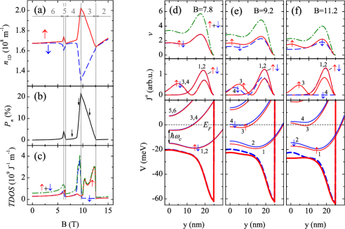
Figure 5: (Color online). 1D charge density for spin-up and spin-down electrons (a), the charge spin polarization (b), the $TDOS$ for spin-up and spin-down electrons, total $TDOS$ (c) as a function of $B$ calculated within the DFT approximation for a narrow wire. (d)-(f) The subband structure for magnetic fields indicated in (b). Upper panel: electron density profiles (local filling factors) $\nu(y)=n(y)/n_{B}$; middle panel: the current density distribution; lower panel: magnetosubband structure for spin-up and spin-down electrons. Fat solid and dashed lines indicate the total confining potential for respectively spin-up and spin-down electrons. The width of the wire is $a=50$ nm and depth is $V_{0}=-0.2$ eV. Temperature $T=1$K.

III.2 Narrow hard wall quantum wire $\frac{w}{2}\lesssim$ $l_{B}$

Let us now concentrate on the case of a narrow wire whose half-width is comparable to the magnetic length. For our analysis we choose the wire of the width $w$=50 nm and $V_{0}=-0.2$ eV. With these parameters the electron density at the center of the wire is $n_{2D}\approx 6\cdot 10^{15}$ m^-2 and the number of spin-resolved subbands is $N=6$ for $B=0$ T.

Figures 5(a) and (b) show respectively the 1D charge density and the polarization for spin-up and spin-down electrons calculated within the DFT approximation. Let us concentrate on the field interval $7\lesssim B\lesssim 12$, when a number of subbands $3\leq N\leq 4$. In this interval the spin polarization shows a pronounced single-loop pattern. This is in contrast to the case of a wide wire that exhibits a double-loop pattern (see Figs. 2 (a),(b)), where the first loop corresponds to the subband depopulation in the middle of the wire, whereas the second loops corresponds to the subband depopulation in the deep triangular well near the boundary. Note that the width of the this well is of the order of the extension of the wave function given by the magnetic length $l_{B}$. This explain a single-loop structure of the polarization curve for the case of a narrow wire $\frac{w}{2}\lesssim l_{B}$. Indeed, in this case the extension of the triangular well is comparable to the half-width of the wire, such that the well extends in the middle region and there is no separate depopulation for the inner and outer regions of the wire.

The above features of the narrow wire can be clearly traced in the evolution of the magnetosubbands, see Fig. 5. When 6.5 T $\lesssim B\lesssim 8.5$ T 3rd and 4th subbands in the middle of the wire are located beneath $E_{F}-2\pi kT$ and are thus fully occupied. This corresponds to the formation of the incompressible strip in the middle of the wire such that the charge densities of spin-up and spin-down electrons are equal (i.e. the spin polarization is zero). At $B=8.5$T 4th subband reaches $E_{F}-2\pi kT$ and thus becomes partially occupied. As a result, the exchange interactions generates spin splitting, and the compressible strip due to spin-down electrons belonging to 4th subband starts to form in the middle of the wire. Spin polarization grows rapidly until it reaches its maximum $P_{n}=22$ %. At this moment 4th subband depopulates and the corresponding compressible strip disappears. When magnetic field is increased only slightly, 3rd subband is raised to $E_{F}-2\pi kT$ and the compressible strip due to spin-up electrons forms in the middle of the wire. Note that formation and disappearance of the compressible strips due to spin-up and spin-down electrons is clearly reflected in the $TDOS$, see Fig. 5(c) which shows peaks belonging to different spin species. With further increase of $B$ the spin polarization decreases linearly until it vanishes when 3rd subband fully depopulates.

Magnetosubband evolution calculated within the Hartree approximation (not shown) qualitatively resembles evolution for the DFT case. In particular, the spin density polarization follows the same behavior reaching the maximum value $P_{n}=10$ in the interval $3\leq N\leq 4$. The similarity between the Hartree and DFT approximations is because of a large Zeeman term for magnetic field intervals under consideration which causes a relatively strong Zeeman splitting in the Hartree approximation.

IV Conclusion

We provide a systematic quantitative description of the structure of the edge states and magnetosubband evolution in hard wall quantum wires in the integer quantum Hall regime. Our calculations are based on the self-consistent Green’s function techniqueIhnatsenka where the electron- and spin interactions are included within the density functional theory in the local spin density approximation. Our main findings can be summarized as follows.

1) The magnetosubband structure and the density distribution in the hard-wall quantum wire is qualitatively different from that one with a smooth electrostatic confinement. In particularly, in the hard-wall wire a deep triangular potential well of the width $\sim l_{B}$ is formed in the vicinity of the wire boundary. The wave functions are strongly localized in this well which leads to the increase of the electron density near the edges.

2) Because of the presence of the deep triangular well near the wire boundaries, the subbands start to depopulate from the central region of the wire and remain pinned in the well region until they are eventually pushed up by an increasing magnetic field. This is in contrast to the case of a smooth confinement where depopulation of the subbands starts from the edges and extends towards the wire center as the magnetic field increases.

3) The spin polarization of electron density as a function of magnetic field shows a pronounced double-loop pattern that can be related to the successive depopulation of the magnetosubbands.

4) In contrast to the case of a smooth confinement, in the hard-wall wires the compressible strips do not form in the vicinity of wire boundaries and a spatial spin separation between spin-up and spin-down states near the edges is absent.

- (1) J. Cibert, P. M. Petroff, G. J. Dolan, S. J. Pearton, A. C. Gossard, J. H. English, Appl. Phys. Lett. 49, 1275 (1986).
- (2) F. E. Prins, G. Lehr, M. Burkard, H. Schweizer, M. H. Pilkuhn, G. W. Smith, Appl. Phys. Lett. 62, 1365 (1993).
- (3) L. N. Pfeiffer, K. W. West, H. L. Eisenstein, K. W. Baldwin, D. Gershoni, J. Spector, Appl. Phys. Lett. 56, 1697 (1990).
- (4) A. Yacoby, H. L. Stormer, K. W. Baldwin, L. N. Pfeifer, K. W. West, Solid State Commun. 101, 77 (1997).
- (5) A. Yacoby, H. L. Stormer, N. S. Wingreen, L. N. Pfeiffer, K. W. Baldwin, K. W. West, Phys. Rev. Lett. 77, 4612 (1996).
- (6) J. Motoshita and H. Sakaki, Appl. Phys. Lett. 63, 1786 (1993).
- (7) M. Huber, M. Grayson, M. Rother, W. Biberacher, W. Wegscheider, and G. Abstreiter, Phys. Rev. Lett. 94, 016805 (2005).
- (8) T. Shitara, M. Tornow, A. Kurtenbach, D. Weiss, K. Ebert, and K. v. Klitzing, Appl. Phys. Lett. 66, 2385 (1995).
- (9) B. I. Halperin, Phys. Rev. B 25, 2185 (1982).
- (10) D. B. Chklovskii, B. I. Shklovskii, and L. I. Glazman, Phys. Rev. B 46, 4026 (1992); D. B. Chklovskii, K. A. Matveev, and B. I. Shklovskii, Phys. Rev. B 47, 12605 (1993).
- (11) J. M. Kinaret and P. A. Lee, Phys. Rev. B 42 11768 (1990).
- (12) T. Suzuki and T. Ando, J. Phys. Soc. Japan 62 2986 (1993).
- (13) J. Dempsey, B. Y. Gelfand, and B. I. Halperin, Phys. Rev. Lett. 70, 3639 (1993).
- (14) L. Brey, J. J. Palacios, and C. Tejedor, Phys. Rev.B 47, 13884 (1993).
- (15) K. Lier and R. R. Gerhardts, Phys. Rev. B 50, 7757 (1994).
- (16) Y. Tokura and S. Tarucha, Phys. Rev. B 50, 10981 (1994).
- (17) T. H. Stoof and G. E. W. Bauer, Phys. Rev. B 52, 12143 (1995).
- (18) M. Ferconi, M. R. Geller, and G. Vignale, Phys. Rev. B 52, 16357 (1995).
- (19) O. G. Balev and P. Vasilopoulos, Phys. Rev. B 56, 6748 (1997); Z. Zhang and P. Vasilopoulos, Phys. Rev. B 66, 205322 (2002).
- (20) T. Suzuki and T. Ando, Physica B 249-251, 415 (1998).
- (21) D. Schmerek and W. Hansen, Pnys. Rev. B 60, 4485 (1999).
- (22) A. Siddiki and R. R. Gerhardts, Phys. Rev. B 70, 195335 (2004).
- (23) S. Ihnatsenka and I. V. Zozoulenko, Phys. Rev. B 73, 075331 (2006).
- (24) S. Ihnatsenka and I. V. Zozoulenko, Phys. Rev. B 73, 155314 (2006).
- (25) R. G. Parr and W. Yang, Density-Functional Theory of Atoms and Molecules, (Oxford Science Publications, Oxford, 1989).
- (26) W. Kohn and L. Sham, Phys. Rev. 140, A1133 (1965).
- (27) M. Ferconi and G. Vignale, Phys. Rev. B 50, R14722 (1994).
- (28) E. Räsänen, H. Saarikoski, V. N. Stavrou, A. Harju, M. J. Puska, and R. M. Nieminen, Phys. Rev B 67, 235307 (2003).
- (29) S. M. Reimann and M. Manninen, Rev. Mod. Phys. 74, 1283 (2002).
- (30) B. Tanatar and D. M. Ceperley, Phys. Rev. B 39, 5005, (1989).
- (31) J. Davies, The Physics of Low-Dimensional Semiconductors, (Cambridge University Press, Cambridge, 1998).
- (32) A. Manolescu and R. R. Gerhardts, Phys. Rev. B 51, 1703 (1995).
- (33) S. Datta, Electronic Transport in Mesoscopic Systems, (Cambridge University Press, Cambridge, 1997).
- (34) D. Weiss, C. Zhang, R. R. Gerhardts, K. v. Klitzing, G. Weimann, Phys. Rev. B 39, 13020 (1989).
- (35) K.-F. Berggren, G. Roos, and H. van Houten, Phys. Rev. B 37, 10 118 (1998).
- (36) S. W. Hwang, D. C. Tsui, and M. Shayegan, Phys. Rev. B 48, 8161 (1993).
- (37) C. W. J. Beenakker, H. van Houten, in Solid State Physics: Advances in Research and Applications, edited by H. Ehrenreich and D. Turnbull (Academic Press, New York, 1991), Vol. 44.