A theoretical analysis on highly spin-polarized transport of iron nitride Fe₄N

Abstract

In order to propose a ferromagnet exhibiting highly spin-polarized transport, we theoretically analyzed the spin polarization ratio of the conductivity of the bulk Fe₄N with a perovskite type structure, in which N is located at the body center position of fcc-Fe. The spin polarization ratio is defined by $P=(\sigma_{\uparrow}-\sigma_{\downarrow})/(\sigma_{\uparrow}+\sigma_{\downarrow})$, with $\sigma_{\uparrow(\downarrow)}$ being the conductivity at zero temperature of the up spin (down spin). The conductivity is obtained by using the Kubo formula and the Slater-Koster tight binding model, where parameters are determined from the least-square fitting of the dispersion curves by the tight binding model to those by the first principles calculation. In the vicinity of the Fermi energy, $|P|$ takes almost 1.0, indicating perfectly spin-polarized transport. In addition, by comparing Fe₄N to fcc-Fe (Fe₄N₀) in the ferromagnetic state with the equilibrium lattice constant of Fe₄N, it is shown that the non-magnetic atom N plays an important role in increasing $|P|$.

Recently, highly efficient spin-electronics devices operating at room temperature have been extensively developed for applications to the magnetic memory and the magnetic sensor. A typical device has ferromagnetic tunnel junctions consisting of a ferromagnetic electrode (FME)/insulator/FME, which exhibits a large magnetoresistance (MR) effect. Inomata ; Sakuraba ; Yuasa1 ; Yuasa2 ; Hayakawa1 ; Hayakawa2 ; Kokado The efficiency of the MR effect is often defined by ${\rm the~{}MR~{}ratio}=(R_{\mbox{\tiny AP}}-R_{\mbox{\tiny P}})/R_{\mbox{\tiny AP}}$, with $R_{\mbox{\tiny P}}$ and $R_{\mbox{\tiny AP}}$ being the resistance of the parallel and anti-parallel magnetization configurations of FMEs, respectively. Experimentally, regarding junctions with an electrode of a half-metallic ferromagnet, Co₂Cr_0.6Fe_0.4Al/Al-O/CoFe/NiFe/IrMn/Ta junctions exhibited an MR ratio of 16 % at room temperature, Inomata and Co₂MnSi/Al-O/Co₇₅Fe₂₅ had an MR ratio of 70 % at room temperature. Sakuraba Regarding junctions of electrodes with usual ferromagnets, single-crystal Fe(001)/MgO(001)/Fe(001) junctions exhibited MR ratios of 88 % Yuasa1 and 180 % Yuasa2 at room temperature. Furthermore, CoFeB/MgO/CoFeB junctions achieved MR ratios of 260 % Hayakawa1 and 355 % Hayakawa2 (the world’s highest value) at room temperature, although the crystal structure of CoFeB and the role of the light element B on the spin-polarized transport have not been clarified yet. Generally, the MR ratio becomes large with increasing the spin polarization of the conduction electron in the FME. In the future, an FME with more highly spin-polarized electrons, which would result in larger MR ratios, will be strongly desired from the viewpoint of the development of highly efficient MR devices.

Towards proposal of such an FME, we extracted an idea to obtain electrodes exhibiting the highly spin-polarized transport at room temperature. We found that ferromagnets consisting of $magnetic~{}elements$ and $light~{}elements$, such as CoFeB, might be very useful as the electrodes.

We consider Fe as a representative magnetic element in this idea. We define the spin polarization (SP) ratio about the density of states (DOS) of the bulk system, $P_{\mbox{\tiny DOS}}(E)$, as

$$P_{\mbox{\tiny DOS}}(E)=\frac{D_{\uparrow}(E)-D_{\downarrow}(E)}{D_{\uparrow}(E)+D_{\downarrow}(E)},$$ (1)

with $D_{s}(E)$ being the DOS of spin $s$ (=$\uparrow$ or $\downarrow$) for the energy $E$. Then, $|P_{\mbox{\tiny DOS}}(E_{\mbox{\tiny F}})|$ at the Fermi energy $E_{\mbox{\tiny F}}$ of fcc-Fe in the ferromagnetic state is evaluated to be about 0.7 [see Fig. 2(c)], which is about 2.3 times as large as that of bcc-Fe, bcc-Fe where the most stable state of bcc-Fe (fcc-Fe) is ferromagnetic (not ferromagnetic Hoshino ). This may indicate that the highly spin-polarized transport is realized for materials closely related to fcc-Fe. The conductivity, including the velocity of electrons, will give an answer to the realizability of such transport.

We focus on a ferromagnet containing fcc-Fe and a light element, Fe₄N with a perovskite-type structure, Jack ; Shirane ; Nagakura ; Zhou ; Sakuma ; Ishida in which N is located at the body center position of fcc-Fe. This ferromagnet has a Curie temperature of 761 K. Nagakura It should be noted that studies on the spin-polarized transport of Fe₄N have scarcely been performed so far, although other properties have been experimentally Jack ; Shirane ; Nagakura and theoretically Zhou ; Sakuma ; Ishida investigated. We are particularly interested in not only the SP ratio on the transport of Fe₄N but also the role of the light (or non-magnetic) element N on the transport.

In this paper, we analyzed the SP ratio of conductivity of Fe₄N in order to elucidate the spin-polarized transport. The conductivity was obtained for each spin and each orbital of the bulk system using the first principles (FP) calculation and the tight binding (TB) model calculation. Consequently, we found that Fe₄N exhibits an extremely highly spin-polarized transport and that N plays an important role in the transport.

A calculation method is introduced to obtain the conductivity and the SP ratio. The method is a combination of (i) the FP calculation, Kresse (ii) the TB model, Slater and (iii) the Kubo formula. Kubo Details of each are given below:

• The FP calculations are performed by the Vienna Ab-initio Simulation Package (VASP) code Kresse based on the spin-polarized density functional theory, where we employ the generalized gradient approximation of Perdew and Wang (PW91) Perdew and ultrasoft pseudopotentials to describe the core electrons. The cutoff energy for the plane wave basis is 237.51 eV for Fe and 348.10 eV for Fe₄N, and the Monkhorst-Pack set Monkhorst of 8$\times$8$\times$8 ${\bf k}$ points is used.

• The Slater-Koster TB model Slater is used with taking into account the 3d, 4s, and 4p orbitals for Fe and the 2s and 2p orbitals for N as well as interactions up to the third-nearest neighbor atoms. The Slater-Koster parameters of potential energies and transfer integrals Slater are here determined from the least-square fitting of the dispersion curves by the TB model to those by the FP calculation at the equilibrium lattice constant. The fitting is done in energy regions from the lowest energy to $E_{\mbox{\tiny F}}$ + 5 eV for bcc-Fe and fcc-Fe and from the lowest energy to $E_{\mbox{\tiny F}}$ + 2 eV for Fe₄N. The number of parameters is 34 for bcc-Fe and fcc-Fe and 87 for Fe₄N.

• The Kubo formula Kubo and the Slater-Koster TB model with the determined parameters are used to calculate the conductivity at zero temperature. In this calculation, we utilize the theory given by Tsymbal et al. Tsymbal The total conductivity of spin $s$ (=$\uparrow$ or $\downarrow$), $\sigma_{s}(E)$, is written by,

  $$\sigma_{s}(E)=\displaystyle{\sum_{i}}\sigma_{i,s}(E),$$ (2)

  where $\sigma_{i,s}(E)$ is the conductivity of orbital $i$ (=4s, 4p, 3d orbitals, and so on) and spin $s$. This $\sigma_{i,s}(E)$ includes the velocity of electrons and the Green’s function. The Green’s function has a single parameter $\gamma$ in the second-order self energy due to the weak electron-impurity interaction, where $\gamma$ characterizes the degree of electron-impurity scattering. In detail, $\gamma$ is related to the lifetime of the electron of orbital $i$ and spin $s$, $\tau_{i,s}$, via $1/\tau_{i,s}=(2\pi/\hbar)\gamma^{2}D_{i,s}(E)$, with $D_{i,s}(E)$ being the partial DOS for $i$ and $s$. Tsymbal At present, $\gamma$ is set to be 0.5 eV, which was previously chosen so as to reproduce the resistivity of copper. Tsymbal We also use the diagonal approximation for the self energy, in which the scattering of electrons due to impurities is allowed for the same energy levels but forbidden between different energy levels. Tsymbal The SP ratio is then defined by

  $$P(E)=\frac{\sigma_{\uparrow}(E)-\sigma_{\downarrow}(E)}{\sigma_{\uparrow}(E)+\sigma_{\downarrow}(E)}.$$ (3)

We first compare the results of bcc-Fe by the present method with the previous ones. The equilibrium lattice constant obtained by using the FP calculation is estimated to be 2.84 Å  with an error of about 1 % for the experimental value of 2.87 Å. Kittel The total conductivity at $E_{\mbox{\tiny F}}$ of the down spin $\sigma_{\downarrow}(E_{\mbox{\tiny F}})$ is larger than $\sigma_{\uparrow}(E_{\mbox{\tiny F}})$. The SP ratio at $E_{\mbox{\tiny F}}$, $P(E_{\mbox{\tiny F}})$, therefore takes a negative value, $-$0.20, and it qualitatively agrees with the previous result of about $-$0.26, Tsymbal which was obtained by a similar method combined with the FP calculation within the local density approximation.

In the following, we investigate the equilibrium lattice constant, $D_{s}(E)$, and $P_{\mbox{\tiny DOS}}(E)$ for Fe₄N using the FP calculation. The equilibrium lattice constant is evaluated as 3.810 Å, which has an error of less than 1 % for an experimental value of 3.795 Å. Nagakura As shown in Figs. 1(a) and 1(c), $D_{\downarrow}(E_{\mbox{\tiny F}})$ is higher than $D_{\uparrow}(E_{\mbox{\tiny F}})$. Partial DOSs Sakuma schematically illustrated in Fig. 1(b) show that 3d orbitals are dominant around $E_{\mbox{\tiny F}}$, and 4s and 4p (4s-4p) orbitals are mainly located in an energy region higher than $E_{\mbox{\tiny F}}$, while each orbital of N atoms mostly exists in an energy region lower than $E_{\mbox{\tiny F}}$. Furthermore, $P_{\mbox{\tiny DOS}}(E_{\mbox{\tiny F}})$ obtained by using $D_{s}(E_{\mbox{\tiny F}})$ of the FP calculation is evaluated to be $-$0.6 [see Fig. 1(c)].

Using the TB model with the parameters determined from the fitting of the dispersion curves, we obtain $D_{s}(E)$ and $P_{\mbox{\tiny DOS}}(E)$ for $-1~{}{\rm eV}\leq E\leq 1~{}{\rm eV}$. As seen from Fig. 1(c), $D_{s}(E_{\mbox{\tiny F}})$ and $P_{\mbox{\tiny DOS}}(E_{\mbox{\tiny F}})$ of the TB model agree well with the respective ones of the FP calculation.

With the use of the TB model and the Kubo formula we calculate $\sigma_{i,s}(E)$, $\sigma_{s}(E)$, and $P(E)$ for $-1~{}{\rm eV}\leq E-E_{\mbox{\tiny F}}\leq 1~{}{\rm eV}$. The results are shown in Fig. 1(d). For $E\leq E_{\mbox{\tiny F}}$, $\sigma_{\mbox{\tiny 3d},\uparrow}(E)$ becomes relatively large owing to the high DOS of the 3d orbitals of the up spin. For $E-E_{\mbox{\tiny F}}\geq 0.6~{}{\rm eV}$, the 4s-4p orbitals of the up spin contribute strongly to $\sigma_{\uparrow}(E)$ in spite of their low DOSs because their orbitals have large velocities. For $0~{}{\rm eV}<E-E_{\mbox{\tiny F}}<0.6~{}{\rm eV}$, each $\sigma_{i,\uparrow}(E)$ has a pronounced valley reflecting the low DOS of the up spin. In this energy region, although the DOS of the up spin is actually lower than that of the FP calculation, the qualitative behavior of $\sigma_{i,\uparrow}(E)$ appears to be valid because the DOS of the FP calculation has very few components of the 4s-4p orbitals and it is low. On the other hand, each $\sigma_{i,\downarrow}(E)$ is almost flat, and the 3d orbitals of the down spin contribute largely to $\sigma_{\downarrow}(E)$ because of their high DOS. The total conductivity at $E_{\mbox{\tiny F}}$ of the down spin $\sigma_{\downarrow}(E_{\mbox{\tiny F}})$ is much larger than $\sigma_{\uparrow}(E_{\mbox{\tiny F}})$. The SP ratio $P(E_{\mbox{\tiny F}})$ therefore takes almost $-$1.0, indicating perfectly spin-polarized transport. The magnitude of the SP ratio $|P(E_{\mbox{\tiny F}})|$ is about 5.0 times as large as that of bcc-Fe.

(a)

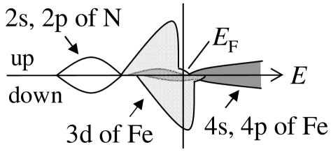
(b)

(c)

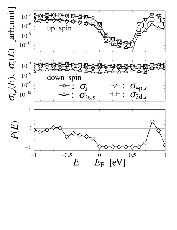
(d)

Figure 1: Density of states, conductivities, and spin polarization ratios of Fe₄N: (a) $D_{s}(E)$ calculated using the FP calculation. (b) Schematic illustration of partial DOSs. The 4s-4p components are partly covered by the 3d ones [see darkish parts in 3d components]. (c) $D_{s}(E)$ and $P_{\mbox{\tiny DOS}}(E)$ for $-1~{}{\rm eV}\leq E-E_{\mbox{\tiny F}}\leq 1~{}{\rm eV}$ of the TB model and the FP calculation. (d) $\sigma_{i,s}(E)$, $\sigma_{s}(E)$, and $P(E)$ for $-1~{}{\rm eV}\leq E-E_{\mbox{\tiny F}}\leq 1~{}{\rm eV}$. Here, $\sigma_{\mbox{\tiny 2s},s}(E)$ and $\sigma_{\mbox{\tiny 2p},s}(E)$ for N are not shown because of their small values.

(a)

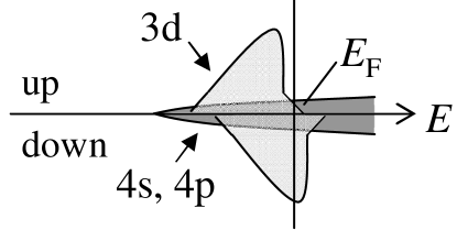
(b)

(c)

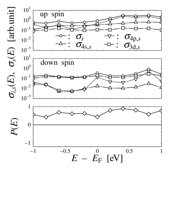
(d)

Figure 2: The same as Fig. 1 for fcc-Fe (Fe₄N₀) in the ferromagnetic state with the equilibrium lattice constant of Fe₄N: (a) $D_{s}(E)$ calculated using the FP calculation. (b) Schematic illustration of partial DOSs. The 4s-4p components are partly covered by the 3d ones [see darkish parts in 3d components]. (c) $D_{s}(E)$ and $P_{\mbox{\tiny DOS}}(E)$ for $-1~{}{\rm eV}\leq E-E_{\mbox{\tiny F}}\leq 1~{}{\rm eV}$ of the TB model and the FP calculation. (d) $\sigma_{i,s}(E)$, $\sigma_{s}(E)$, and $P(E)$ for $-1~{}{\rm eV}\leq E-E_{\mbox{\tiny F}}\leq 1~{}{\rm eV}$.

In order to clarify the effect of an N atom on the transport, we investigated $D_{s}(E)$, $P_{\mbox{\tiny DOS}}(E)$, $\sigma_{i,s}(E)$, $\sigma_{s}(E)$, and $P(E)$ of fcc-Fe (Fe₄N₀) in the ferromagnetic state with an equilibrium lattice constant of Fe₄N. Regarding $D_{s}(E)$ around $E_{\mbox{\tiny F}}$ obtained using the FP calculation, $D_{\downarrow}(E)$ is much higher than $D_{\uparrow}(E)$ [see Figs. 2(a) and 2(c)]; for further details, low and broad DOSs of the 4s-4p orbitals of the up spin and a high DOS of the 3d orbitals of the down spin are observed [see Fig. 2(b)]. The SP ratio of DOS, $P_{\mbox{\tiny DOS}}(E_{\mbox{\tiny F}})$, is evaluated to be about $-$0.7. Figure 2(c) also shows $D_{s}(E)$ and $P_{\mbox{\tiny DOS}}(E)$ for $-1~{}{\rm eV}\leq E\leq 1~{}{\rm eV}$; these values are obtained using the TB model with the determined parameters. It is found that $D_{s}(E_{\mbox{\tiny F}})$ and $P_{\mbox{\tiny DOS}}(E_{\mbox{\tiny F}})$ of the TB model agree fairly well with the respective ones of the FP calculation. With the use of the TB model, we calculate $\sigma_{i,s}(E)$ and $\sigma_{s}(E)$ [see Fig. 2(d)]. In spite of the low DOSs of the 4s-4p orbitals of the up spin, their orbitals contribute strongly to $\sigma_{\uparrow}(E)$. This tendency originates from the large velocities of the 4s-4p orbitals. Moreover, $\sigma_{\mbox{\tiny 3d},\downarrow}(E)$ is relatively large reflecting the high DOS of the 3d orbitals of the down spin. The total conductivity at $E_{\mbox{\tiny F}}$ of the up spin $\sigma_{\uparrow}(E_{\mbox{\tiny F}})$ then becomes larger than $\sigma_{\downarrow}(E_{\mbox{\tiny F}})$ even though $D_{\uparrow}(E_{\mbox{\tiny F}})$ is much lower than $D_{\downarrow}(E_{\mbox{\tiny F}})$. The SP ratio $P(E_{\mbox{\tiny F}})$ has a positive sign, opposite to the sign of $P_{\mbox{\tiny DOS}}(E_{\mbox{\tiny F}})$. This sign of $P(E_{\mbox{\tiny F}})$ is also opposite to that of Fe₄N. The magnitude of the SP ratio $|P(E_{\mbox{\tiny F}})|$ is evaluated to be 0.4, which is between the $|P(E_{\mbox{\tiny F}})|$ of Fe₄N and that of bcc-Fe.

On the basis of the above investigations and the evaluated Slater-Koster parameters, we discuss the role of the N atom on the highly spin-polarized transport of Fe₄N using schematic illustrations of partial DOSs [see Figs. 1(b) and 2(b)]. Note that by merely introducing the non-magnetic atom N to the body center position of fcc-Fe, $|P(E_{\mbox{\tiny F}})|$ becomes about 2.5 times as large as that of fcc-Fe and the sign of $P(E_{\mbox{\tiny F}})$ changes. In the present study, we find that, by adding N to fcc-Fe, 4s-4p bands of Fe are raised to a higher energy region by a large magnitude of transfer integrals between the 4s-4p orbitals of Fe and the 2s and 2p orbitals of N, while 3d bands do not change significantly owing to the small magnitude of the transfer integrals between the 3d orbitals of Fe and the 2s and 2p orbitals of N. These behaviors are explained by considering the bonding-antibonding states formed by the transfer integrals, which correspond to overlaps between both orbitals. A large portion of 4s-4p bands exists in an energy region higher than 3d bands, and a small portion of them is located in the energy region of 3d bands because of hybridizations with 3d orbitals, and is then spin-polarized there. Hence, comparing Fe₄N with fcc-Fe, the proportion of 4s-4p bands is small in the vicinity of $E_{\mbox{\tiny F}}$, and, in particular, the proportion of the up spin is extremely small; the 3d bands of the down spin are dominant there. Therefore, the magnitude of the SP ratio $|P(E_{\mbox{\tiny F}})|$ increases, and $P(E_{\mbox{\tiny F}})$ becomes negative.

Finally, although it would be difficult to derive the general properties of phenomena from the present study alone, it seems possible that various ferromagnets consisting of magnetic elements and light elements have a large magnitude of SP ratios according to the same mechanism as that of Fe₄N. In addition, when such ferromagnets are used as the FMEs, FME/insulator/FME junctions may exhibit large MR ratios, although the MR ratios are often influenced by the interfacial states and materials of the insulator. In fact, CoFeB electrodes bring about a very large MR effect in CoFeB/MgO/CoFeB junctions. Hayakawa1 ; Hayakawa2

In conclusion, $|P(E_{\mbox{\tiny F}})|$ of Fe₄N was evaluated to be almost 1.0, which was about 5.0 times as large as that of bcc-Fe and about 2.5 times as large as that of fcc-Fe. In comparison with fcc-Fe, it was shown that the large magnitude of the SP ratio originated from the contribution to the transport of 3d bands, which was enhanced by introducing N. We anticipate that Fe₄N will become an electrode with a high efficiency of spin injection. Furthermore, various ferromagnets consisting of magnetic elements and light elements may exhibit highly spin-polarized transport due to the present mechanism.

The authors thank Prof. T. Hoshino of Shizuoka University for useful discussions. One of the authors (S.K.) also thank members of nanomaterials theory group, AIST, for valuable discussions. This work has been supported by a competitive grant program 2005 of Shizuoka University.

References

- (1) K. Inomata, S. Okamura, R. Goto, and N. Tezuka, Jpn. J. Appl. Phys. 42, L419 (2003).
- (2) Y. Sakuraba, J. Nakata, M. Oogane, H. Kubota, Y. Ando, A. Sakuma, and T. Miyazaki, Jpn. J. Appl. Phys. 44, L1100 (2005).
- (3) S. Yuasa, A. Fukushima, T. Nagahama, K. Ando, and Y. Suzuki, Jpn. J. Appl. Phys. 43, L588 (2004).
- (4) S. Yuasa, T. Nagahama, A. Fukushima, Y. Suzuki, and K. Ando, Nature Mater. 3, 868 (2004).
- (5) J. Hayakawa, S. Ikeda, F. Matsukura, H. Takahashi, and H. Ohno, Jpn. J. Appl. Phys. 44, L587 (2005).
- (6) S. Ikeda, J. Hayakawa, Y. M. Lee, R. Sasaki, T. Meguro, F. Matsukura, and H. Ohno, Jpn. J. Appl. Phys. 44, L1442 (2005).
- (7) S. Kokado and K. Harigaya, Phys. Rev. B 69, 132402 (2004).
- (8) By performing the first principles calculation with the use of Vienna Ab-initio Simulation Package code, we evaluated of bcc-Fe to be about 0.3.
- (9) T. Hoshino, M. Asato, T. Nakamura, R. Zeller, and P. H. Dederichs, J. Magn. Magn. Mater. 272-276, e229 (2004).
- (10) K. H. Jack, Proc. Roy. Soc. London Ser. A 195, 34 (1948).
- (11) G. Shirane, W. J. Takei, and S. L. Ruby, Phys. Rev. 126, 49 (1962).
- (12) S. Nagakura, J. Phys. Soc. Jpn. 25, 488 (1968).
- (13) W. Zhou, L. J. Qu, Q. M. Zhang, and D. S. Wang, Phys. Rev. B 40, 6393 (1989).
- (14) A. Sakuma, J. Phys. Soc. Jpn. 60, 2007 (1991); J. Magn. Magn. Mater. 102, 127 (1991).
- (15) S. Ishida and K. Kitawatase, J. Magn. Magn. Mater. 104-107, 1933 (1992).
- (16) G. Kresse and J. Hafner, Phys. Rev. B 47, R558 (1993); 49, 14251 (1994); G. Kresse and J. Furthmuller, Comput. Mater. Sci. 6, 15 (1996); Phys. Rev. B 54, 11169 (1996).
- (17) J. C. Slater and G. F. Koster, Phys. Rev. 94, 1498 (1954).
- (18) R. Kubo, J. Phys. Soc. Jpn. 12, 570 (1957).
- (19) J. P. Perdew, J. A. Chevary, S. H. Vosko, K. A. Jackson, M. R. Pederson, D. J. Singh, and C. Fiolhais, Phys. Rev. B 46, 6671 (1992).
- (20) H. J. Monkhorst and J. D. Pack, Phys. Rev. B 13, 5188 (1976).
- (21) E. Yu. Tsymbal and D. G. Pettifor, Phys. Rev. B 54, 15314 (1996).
- (22) C. Kittel, Introduction to Solid State Physics, 6th edition (John Wiley & Suns, New York, 1986), p. 23.