Theory of non-Fermi liquid and pairing in electron-doped cuprates

Abstract

We apply the spin-fermion model to study the normal state and pairing instability in electron-doped cuprates near the antiferromagnetic QCP. Peculiar frequency dependencies of the normal state properties are shown to emerge from the self-consistent equations on the fermionic and bosonic self-energies, and are in agreement with experimentally observed ones. We argue that the pairing instability is in the $d_{x^{2}-y^{2}}$ channel, as in hole-doped cuprates, but theoretical $T_{c}$ is much lower than in the hole-doped case. For the same hopping integrals and the interaction strength as in hole-doped materials, we obtain $T_{c}\sim 10$K at the end point of the antiferromagnetic phase. We argue that a strong reduction of $T_{c}$ in electron-doped cuprates compared to hole-doped ones is due to critical role of the Fermi surface curvature for electron-doped materials. The $d_{x^{2}-y^{2}}$-pairing gap $\Delta(\mathbf{k},\omega)$ is strongly non-monotonic along the Fermi surface. The position of the gap maxima, however, does not coincide with the hot spots, as the non-monotonic $d_{x^{2}-y^{2}}$ gap persists even at doping when the hot spots merge on the Brillouin zone diagonals.

PACS: 74.25.-q, 74.20.Mn

I Introduction

The fascinating properties of high-temperature superconductors continue to attract high interest of condensed-matter community over the last two decades. Most of the extensive experimental and theoretical studies of the cuprates have been performed on hole-doped materials, such as La_2-xSr_xCuO₄, YBa₂Cu₃O_6+x (YBCO), Bi₂Sr₂CaCu₂O_8+x(Bi-2212), Tl₂Ba₂CuO_6+x, etc. In recent years, however, there has been growing interest in the properties of electron-doped cuprates such as Nd_2-xCe_xCuO₄ and Pr_2-xCe_xCuO₄ damascelli ; blumberg02 .

Hole-doped and electron-doped cuprates are in many respects similar. For both, optical conductivity measurements at small doping show a charge-transfer gap of about $2$eV basov ; onose04 , and the electronic Fermi surface, measured by ARPES in electron-doped cuprates is reasonably described the same combination of hopping integrals as in hole-doped cuprates damascelli . This implies that both electron-doped and hole-doped materials are likely described by the same underlying Hubbard-type model millis04 . The normal state behavior of optical conductivity near optimal doping is also very similar in hole-doped and electron-doped materials  marel ; homes . Most importantly, the superconductivity in both types of materials has $d_{x^{2}-y^{2}}$ symmetry, as evidenced by, e.g., ARPES measurements of the momentum dependence of the pairing gap camp ; sato .

On the other hand, the phase diagrams of hole-doped and electron-doped cuprates are somewhat different. Electron-doped cuprates have a much wider range of antiferromagnetism than hole-doped materials el-pd ; Aiff03 . There is a strong evidence that the Mott physics is not very relevant in electron-doped cuprates near optimal doping as the optical data show onose04 that the $1.7$eV charge-transfer gap completely melts away as the electron doping approaches its optimal value $x\sim 0.15$. There is also no analog in electron-doped cuprates of the pseudogap phase between the antiferromagnetic and superconducting phases on the phase diagram. Some pseudogap behavior in the normal state has been detected in Nd_1.85Ce_0.15CuO₄, but the onset temperature for this behavior clearly tracks the Neel temperature  koitzsch03 , and so a (narrow) pseudogap phase is likely just a magnetic fluctuation regime of a quasi-2D antiferromagnet zimmers05 . In the absence of the pseudogap, the phase diagram of electron-doped cuprates resembles a “typical” quantum-critical phase diagram piers - the superconducting $T_{c}(x)$ forms a dome above the antiferromagnetic quantum-critical point (QCP) dagan04 .

The superconducting properties of the two classes of materials also differ. First, $T_{c}$ in electron-doped cuprates is around $10-20$K which is almost an order of magnitude smaller than in hole-doped cuprates, and up to a factor $500$ smaller than the pseudogap $T^{*}$, which, as a large group of researchers believe, is the onset temperature of the pairing without coherence in hole-doped cuprates. Second, the pairing gap in electron-doped cuprates varies non-monotonically along the Fermi surface – it increases at deviations from Brillouin zone diagonals, passes through a maximum, and then decreases. The non-monotonic behavior of the $d-$wave gap has been originally introduced to explain Raman data blumberg02 . Later, the non-monotonic gap has been directly observed in ARPES experiments  blumberg02 ; sato . In hole-doped cuprates, the $d-$wave gap is monotonic, within error bars camp .

The large difference between $T_{c}$ in electron and hole-doped cuprates (and even larger difference with $T^{*}$ for the hole-doped materials) despite apparently similar hopping integrals and the strength of the Hubbard interaction calls for an explanation. In this paper, we argue that the primary difference between the pairing instability temperature in electron-doped and hole-doped materials is that in hole-doped cuprates the pairing predominantly involves antinodal fermions, while for electron doped cuprates the pairing involves fermions near zone diagonals. We show that for the pairing of near-diagonal fermions, the Fermi surface curvature has a very strong and negative effect on $T_{c}$, and reduces it by more than two orders of magnitude. This eventually leads to $T_{c}\sim 10$K in electron-doped cuprates.

To solve the pairing problem, one needs to select a pairing mechanism. Following earlier works by one of us and the others  pines-scalapino ; manske00 ; abanov03 , we assume that the pairing is of electron rather than phonon origin, and that a dominant pairing interaction between fermions is mediated by collective, Landau-overdamped magnetic fluctuations. The idea of spin-fluctuation pairing was earlier applied to hole-doped cuprates, with the assumption that Mott physics does not play a substantial role in the normal (not pseudogap) state, and becomes relevant only well inside the pseudogap phase. For hole-doped cuprates, the Luttinger Fermi surface is such that the hot spots (Fermi surface points separated by the antiferromagnetic momentum) are located near the corners of the Brillouin zone. The pairing near a QCP predominantly involves fermions from around the hot spots, and the region of pairing instability forms a dome on top of the antiferromagnetic QCP abanov03 . The instability temperature increases with underdoping and saturates at $T^{*}\sim 0.03{\bar{g}}$ finn , where ${\bar{g}}$ is the effective interaction, which is comparable to the charge transfer gap. Using $1.5$eV for ${\bar{g}}$ yields $T^{*}\sim 500$K, which is consistent with the onset temperature for the pseudogap behavior. The relation between $T^{*}$ and the actual $T_{c}$ is a separate issue which we will not discuss in this paper.

We will apply the same itinerant spin-fermion model to study the spin-mediated pairing in electron-doped cuprates. Like we said, the electron-doped cuprates seem even more suitable for an itinerant description than the hole-doped materials as there is no non-magnetic pseudogap, and the charge-transfer gap melts away near optimal electron doping. We assume, following RPA studies of the static spin susceptibility, that antiferromagnetism sets in at around the doping when the hot spots merge on the Brillouin zone diagonals manske00 ; markiewicz03 ; onufrieva04 . At this doping the antiferromagnetic Brillouin zone touches the Fermi surface at the diagonal points $\mathbf{k}_{F}=(\pi/2,\pi/2)$ (see Fig. 1), so that $2\mathbf{k}_{F}$ coincides with the antiferromagnetic wave vector $\mathbf{Q}$. At smaller dopings, the system is magnetically ordered, and the fermionic Fermi surface displays electron and hole pockets.

We first consider normal state properties near a $2k_{F}$ antiferromagnetic QCP. We reproduce and extend earlier result of Altshuler, Ioffe, and Millis altshuler95 that at QCP, the self-energy of a nodal fermion has a non-Fermi liquid form and scales as $\Sigma(\omega)\propto\omega^{a}$. The exponent $a$ is close to unity though itself varies with frequency. In this situation, the normal state behavior is close to that in a marginal Fermi liquid.

We next consider the pairing of these non-Fermi liquid fermions and show that at QCP, the system is still unstable towards $d_{x^{2}-y^{2}}$ gap opening, i.e., there is a dome of the pairing instability around critical doping where antiferromagnetism sets in. The pairing instability temperature at QCP (which for electron-doped systems we will label as $T_{c}$ because of the absence of the pseudogap) still scales with ${\bar{g}}$ but because of the strong de-pairing effect associated with the Fermi surface curvature, $T_{c}\sim 0.0006{\bar{g}}$ for the actual curvature of the cuprates Fermi surface. This is 50 times smaller than $0.03{\bar{g}}$ for hole-doped cuprates. The uncertainty of $T_{c}$ due to the approximate nature of the estimate of the curvature is actually very weak as $T_{c}$ as a function of the curvature is almost flat in a wide range of the curvatures.

We also show that the pairing gap is non-monotonic along the Fermi surface, and passes through a maximum at some deviation from the zone diagonal. The location of the gap maxima does not track hot spots as at $2k_{F}$ QCP, the hot spots are right along the zone diagonals.

That an antiferromagnetically mediated $d_{x^{2}-y^{2}}$ pairing survives in a situation when the hot spots are along the zone diagonals is not intuitively obvious, for the strongest pairing interaction involves quasiparticles for which the $d_{x^{2}-y^{2}}$ superconducting gap vanishes. However, one can easily see that the separation between the near-nodal fermions with opposite signs of the $d_{x^{2}-y^{2}}$ gap is on average closer to $\mathbf{Q}$ than that between fermions with the same sign of the gap (see Fig. 1 b). Because of this difference, there is still attraction in the $d_{x^{2}-y^{2}}-$wave channel for the spin-fluctuation mediated interaction. Furthermore, we will see that for the pairing at QCP, the kernel of the gap equation actually does not have any extra smallness associated with the hot spots location along the zone diagonals, i.e., $T_{c}$ is formally of order ${\bar{g}}$. This happens because the gap equation relates $\Delta(\mathbf{k})$ near the two diagonal hot spots $\mathbf{k}_{F}$ and $\mathbf{k}_{F}+\mathbf{Q}$ on the Fermi surface, where both gaps are linear in the deviation from the diagonal. Then the gap equation effectively becomes an equation on the slope of $\Delta(\mathbf{k})$ and the latter one does not contain any extra smallness, as we will see.

The $d_{x^{2}-y^{2}}$ pairing near $2k_{F}$ instability has been earlier considered within BCS theory yakovenko04 , where the authors found that $d-$wave $T_{c}$ remains small but finite at QCP. Our results agree with Ref. yakovenko04 in that the $d-$wave attraction survives at QCP, but we argue that the pairing involves non-Fermi liquid fermions, and that $T_{c}$ scales with the upper boundary of the quantum-critical regime (modulo small prefactor) rather than with the upper boundary of the Fermi liquid behavior. The strong reduction of $T_{c}$ in electron-doped cuprates compared to the onset temperature for the pairing in hole-doped cuprates was also obtained in FLEX studies of magnetically-mediated pairing manske00 (although the difference was less drastic than in our case). We believe that the numerical results of Ref. manske00 describe the same physics as our analysis. Non-monotonic variation of the $d-$wave gap also agrees with recent numerical studies num .

A short summary of our results was presented earlier in krotkov06 .

The paper is organized as follows. In Section II we briefly review the spin-fermion approach. In Section III we study the properties of electron-doped materials in the normal state. In subsection III.1 we develop perturbation approach to fermionic and bosonic self-energies. Self-consistent solution of the Dyson’s equations on the fermionic and bosonic self-energies is covered in subsection III.2. In subsection III.3 we use the obtained self-energy to find the frequency dependences of the conductivity and Raman absorption. In Section IV we address the pairing problem and obtain $T_{c}$ and the momentum dependence of the gap. In IV.1 we consider the limit when the parameter representing curvature of the Fermi surface in the gap equation formally tends to zero. In IV.2 we consider the case of finite curvature. We present numerical solution in IV.2.1, and an approximate analytical solution in IV.2.2, and find that the strong variation of $T_{C}$ with the curvatures can be well understood. In Section V we sum up the main conclusions. Some technical details are relegated to Appendices.

II Model

In this paper we apply the spin-fermion model to a particular form of electron dispersion in two dimensions. In general, low energy dynamics of strongly-interacting electrons may be studied by integrating out the high-energy part of electron-electron interaction. Close to a collective instability, the corresponding bosonic collective mode tends to become gapless, and has to be included in the low-energy model. The interaction with the near-gapless collective mode alters the fermionic dynamics and may lead to non-Fermi-liquid behavior. The same interaction also gives rise to the pairing.

A spin-fermion model has been previously applied to hole-doped cuprates, and we refer the reader to earlier literature abanov03 for the details and the justification of the model. Here we start right with the Hamiltonian:

$$\mathcal{H} = \sum_{\mathbf{k}}\epsilon_{\mathbf{k}}c_{\mathbf{k}\alpha}^{\dagger}c_{\mathbf{k}\alpha}+\sum_{\mathbf{q}}\chi_{0}^{-1}(\mathbf{q})\mathbf{S}_{\mathbf{q}}\mathbf{S}_{-\mathbf{q}}$$ (1)

$$+g\sum_{\mathbf{k},\mathbf{q}}c_{\mathbf{k}+\mathbf{q},\alpha}^{\dagger}\mbox{\boldmath$\sigma$}_{\alpha\beta}c_{\mathbf{k}\beta}\mathbf{S}_{\mathbf{q}},$$

Here $c_{\mathbf{k}}$ are the low-energy fermions and $\mathbf{S}_{\mathbf{q}}$ are their collective bosonic fluctuations in the spin channel. The spin-fermion interaction is described by the effective coupling $g$; self-consistency of the model requires $g$ to be smaller, or, at most, of the order of the bandwidth $g\leq W$. Static spin susceptibility $\chi_{0}(\mathbf{q})$ is determined by the high-energy physics. We assume that it has Ornstein-Zernike form near the antiferromagnetic vector $\mathbf{Q=}(\pi,\pi)$:

$$\chi_{0}(\mathbf{q})=\chi_{0}/(\xi^{-2}+(\mathbf{q}-\mathbf{Q})^{2})$$ (2)

The correlation length $\xi$ parameterizes proximity to the instability. At QCP which we only study below, $\xi^{-1}=0$. The interaction $g$ and $\chi_{0}$ appear only in combination ${\bar{g}}=g^{2}\chi_{0}$ which is the actual (measurable) spin-fermion interaction.

While the static spin susceptibility is an input, the low-frequency dynamic part of the susceptibility (2) should be determined within the model, together with the fermionic self-energy. The reasoning is that the damping of the bosonic fluctuations occurs only by a decay into particle-hole pairs with energies smaller than the bosonic frequency. Because (2) is peaked at the antiferromagnetic wave vector $\mathbf{Q}$, the interaction between fermions and bosons will predominantly involve fermions near the hot spots (Fermi surface points separated by $\mathbf{Q}$).

The computational tool to solve the model of Eq. (1) at large $\xi$ is Eliashberg-type theory in which one solves for fully renormalized fermionic and bosonic self-energies while simultaneously neglecting vertex corrections and the self-energy dependence on momentum transverse to the Fermi surface. This computational procedure is similar, but not equivalent to FLEX. Eliashberg theory at strong coupling has been discussed extensively in early literature abanov03 and we will just use it in our work without further discussion.

III Normal-State Properties

III.1 Perturbation approach

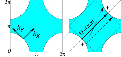
Figure 1: Left: Fermi surface at the antiferromagnetic QCP with $2k_{F}=(\pi,\pi)$. Diamond-shaped dashed lines bound the magnetic Brillouin zone. The diagonal points of the Fermi surface (nodal points of the $d_{x^{2}-y^{2}}$-wave gap) now become “hot”. Right: Graphic explanation of the attraction in the $d_{x^{2}-y^{2}}$ channel: parts of the Fermi surface on the same side of the zone diagonals are on average closer to the $\mathbf{Q}$ separation than the parts on the opposite sides, leading to attraction in the $d_{x^{2}-y^{2}}$ channel (plus and minus are the signs of the $d_{x^{2}-y^{2}}$ gap).

The system behavior at $2k_{F}$ QCP within Eliashberg theory has been studied by Altshuler et al. altshuler95 . They used RG procedure to sum up the most divergent diagrams and obtained fermionic and bosonic self-energies at the lowest frequencies in the normal state. We obtained very similar results using a somewhat different computational procedure (see below). We also obtained fermionic self-energy at intermediate frequencies which are mostly relevant for the pairing problem.

A set of self-consistent Dyson’s equations for the fermionic and bosonic self-energies in the normal state is

$$\chi^{-1}(\mathbf{q},\omega) = \chi_{0}(\mathbf{q})^{-1}+\Pi(\mathbf{q},\omega),$$ (3)

$$G^{-1}(\mathbf{k},\omega) = G_{0}(\mathbf{k},\omega)^{-1}+i\Sigma(\mathbf{k},\omega).$$ (4)

The Green’s function of noninteracting fermions is

$$G_{0}^{-1}(\mathbf{k},\omega)=i\omega-\epsilon_{\mathbf{k}},$$ (5)

and $\epsilon_{\mathbf{k}}$ is the electron dispersion. Bosonic self-energy (polarization operator) contains contributions from non-umklapp and umklapp scattering between hot spots separated by $\mathbf{Q}$. Hereafter we denote by $\mathbf{q}$ the deviation of $\mathbf{q}$ from the antiferromagnetic wave vector $\mathbf{Q}$ unless otherwise noted. In these units, the total polarization operator is $2(\Pi(\mathbf{q},\Omega)+\Pi(-\mathbf{q},\Omega))$, where

$$\Pi(\mathbf{q},\Omega)=2g^{2}\int\frac{d\omega d^{2}\mathbf{k}}{(2\pi)^{3}}G(\mathbf{k},\omega)G(\mathbf{k}+\mathbf{q},\omega+\Omega).$$ (6)

Then

$$\chi(\mathbf{q},\Omega)=\frac{\chi_{0}}{\mathbf{q}^{2}+2\chi_{0}\left(\Pi(\mathbf{q},\Omega)+\Pi(-\mathbf{q},\Omega)\right)}.$$ (7)

The peculiarity of a spin-fermion theory near a $2k_{F}$ instability is that the Fermi velocities at the hot spots are antiparallel, and to keep $\Pi(\mathbf{q},\Omega)$ finite, one has to expand the spectrum of the fermions in the vicinity of these points up to the second order in the momentum component along the Fermi surface:

$$\epsilon_{\mathbf{k}} \approx v_{F}k_{x}+\beta^{2}k_{y}^{2},$$ (8)

$$\epsilon_{\mathbf{k}+\mathbf{Q}} \approx -v_{F}k_{x}+\beta^{2}k_{y}^{2}.$$ (9)

Here the momentum components $k_{x}$, $k_{y}$ are normal and tangential to the Fermi line respectively, and $\mathbf{k}$ is measured from the hot spot (see Fig. 1); $\beta$ parameterizes the curvature of the Fermi line, $\kappa=2\beta^{2}/v_{F}$. The radius of curvature used in altshuler95 is $k_{\kappa}=1/\kappa$. The special case of a nested Fermi surface has been analyzed in  nested A. Virosztek and J. Ruvalds, Phys. Rev. B 42, 4064 (1990).

For noninteracting fermions with the Green’s function (5), Eq. (6) yields

$$\Pi_{0}(\mathbf{q},\Omega)=\frac{g^{2}}{2\pi v_{F}\beta}\sqrt{\sqrt{\Omega^{2}+E_{\mathbf{q}}^{2}}+E_{\mathbf{q}}},$$ (10)

where

$$E_{\mathbf{q}}=-v_{F}q_{x}+\beta^{2}q_{y}^{2}/2.$$ (11)

Already this zeroth-order expression (10) differs in two important ways from previously studied case abanov03 when the two hot spots separated by $\mathbf{Q}$ had nearly orthogonal velocities. First, at $\mathbf{q}=\mathbf{Q}$ $\Pi(\Omega)$ scales as $\sqrt{\Omega}$ instead of the conventional $|\Omega|$, and, moreover, diverges when $\beta\rightarrow 0$ , so curvature of the Fermi line cannot be neglected. Later we will see that $\beta\neq 0$ is even more important for the pairing. It is interesting to trace how (10) converts into a conventional Landau damping when the hot spots are moving away from the zone diagonals. This is done in Appendix A.

Second, a conventional Landau damping $|\Omega|$ term represents an anomaly in analytical properties of bosonic self-energy. External frequency $\Omega$ appears as a factor because it regularizes the integral over internal frequencies by separating the poles into opposite semi-planes. At the same time, the polarization operator (10) gives a fractional power of external frequency not as a result of anomaly, but simply because $\Omega$ sets an effective cutoff for the ultraviolet-divergent integral over internal $\omega$. This distinction becomes relevant at a finite $T$: while Landau damping is a purely quantum phenomenon, and so does not depend on temperature, the self-energy (10) possesses $\omega/T$-scaling. Evaluating the polarization operator for free fermions but at a finite $T$, we obtain

$$\widetilde{\Pi}_{0}(\mathbf{q},\Omega) = \frac{g^{2}}{2\pi v_{F}\beta}\int_{-\infty}^{\infty}\frac{\sqrt{\sqrt{4\omega^{2}+\Omega^{2}}+2\omega}}{4T\cosh^{2}\frac{\omega-E_{\mathbf{q}}/2}{2T}}d\omega$$ (12)

$$= \sqrt{T}f(\Omega/T,E_{\mathbf{q}}/T),$$ (13)

where

$$f(a,b)=\frac{g^{2}}{2\pi v_{F}\beta}\int_{-\infty}^{\infty}\frac{\sqrt{\sqrt{4x^{2}+a^{2}}+2x}}{4\cosh^{2}((x-b)/2)}dx.$$ (14)

At $\mathbf{q}=0$, $\Omega=0$, the polarization operator is simply:

$$\widetilde{\Pi}_{0}=\frac{g^{2}\sqrt{\pi T}}{2\pi v_{F}\beta}|\zeta(\textstyle\frac{1}{2})|(\sqrt{2}-1)=\mathop{\mathrm{const}}\nolimits\sqrt{T},$$ (15)

where $\zeta(\textstyle\frac{1}{2})\approx-1.46$ is the Riemann Zeta function comment . When $T\rightarrow 0$, the function $1/4T\cosh^{2}(x/2T)$ in the denominator of (12) becomes a $\delta(x)$-function, and (12) converts to (10).

The electron self-energy is given by

$$\Sigma(\mathbf{k},\omega)=3ig^{2}\int\frac{d\omega^{\prime}d^{2}\mathbf{k}^{\prime}}{(2\pi)^{3}}\chi(\mathbf{k}-\mathbf{k}^{\prime},\omega-\omega^{\prime})G(\mathbf{k}^{\prime},\omega^{\prime}),$$ (16)

The coefficient $3=\mbox{\boldmath$\sigma$}\mbox{\boldmath$\sigma$}$ in (16) comes from the three components of the bosonic spin fluctuations. In Eliashberg theory, the self-energy depends on frequency and on the momentum component along the Fermi surface. We parameterize the position of the quasiparticle on the Fermi surface by the momentum component $k_{y}$ (see Fig. 1), i.e., label $\Sigma(\mathbf{k},\omega)$ as $\Sigma(k_{y},\omega)$ along the Fermi surface. This does not imply that $k_{x}$ is zero as $k_{x}$ and $k_{y}$ are related: from $\epsilon_{k}=0$, $k_{x}=-\beta^{2}k_{y}^{2}/v_{F}$ along the Fermi surface. Since fermions are fast compared to bosons, the integral over momenta in (16) can be factorized: the one perpendicular to the Fermi surface involves only fast electrons, and the one along the Fermi surface ($\epsilon_{\mathbf{k}^{\prime}}=0$) involves slow bosons. The corrections from keeping the momentum transverse to the Fermi surface in the bosonic propagator is of the same smallness as the vertex correction (in this, Eliashberg theory differs from FLEX where the momentum integration is not factorized)

Substituting

$$G(\mathbf{k},\omega)^{-1}=i(\omega+\Sigma(\mathbf{k},\omega))-\epsilon_{\mathbf{k}}$$ (17)

into (16) and integrating over momenta transverse to the Fermi surface, we obtain for the self-energy

$$\Sigma(k_{y},\omega)=\int_{-\omega}^{\omega}\frac{d\Omega}{2\pi}\int dk^{\prime}_{y}\widetilde{\chi}(k,k^{\prime}_{y},\Omega),$$ (18)

The reduced bosonic propagator

$$\widetilde{\chi}(k_{y},k^{\prime}_{y},\Omega)=\frac{3g^{2}}{4\pi v_{F}}\left.\chi(\mathbf{k}^{\prime}-\mathbf{k},\Omega)\right|_{\epsilon_{\mathbf{k}}=\epsilon_{\mathbf{k}^{\prime}}=0}$$ (19)

is taken between the two points $\mathbf{k}$ and $\mathbf{k}^{\prime}$ on opposite sheets of the Fermi surface.

The reduced propagator depends on the curvature in two ways. First, the polarization operator $\Pi$ depends on curvature via the overall factor and the $E_{\mathbf{q}}$ term in Eq. (11). Second, there is a direct $\beta$ dependence in the static part of the susceptibility, as $(k_{x}-k_{x}^{\prime})^{2}$ term in $\chi$ reduces to $\beta^{4}(k_{y}^{2}+k^{\prime}_{y}{}^{2})^{2}/v_{F}^{2}$ once we use the Fermi surface relations $k_{x}=-\beta^{2}k_{y}^{2}/v_{F}$ and $k^{\prime}_{x}=\beta^{2}k^{\prime}_{y}{}^{2}/v_{F}$.

For the self-energy exactly at the hot spot $(\pi/2,\pi/2)$, the first dependence is much more relevant than the second one. Indeed, setting the external momentum $k=0$ and taking $k^{\prime}$ to be at the Fermi surface we find that $E_{\mathbf{q}}$ and $E_{-\mathbf{q}}$ terms with $\mathbf{q}=\mathbf{k}^{\prime}$ reduce to $E_{\mathbf{k}^{\prime}}=-\beta^{2}k_{y}^{\prime}{}^{2}/2$, and $E_{-\mathbf{k}^{\prime}}=3\beta^{2}k_{y}^{\prime}{}^{2}/2$, i.e., $E_{\pm\mathbf{k}^{\prime}}$ scales with the curvature. The polarization operators $\Pi(\mathbf{q},\Omega)$ and $\Pi(-\mathbf{q},\Omega)$ given by (10) depend on the ratio $\Omega/E_{\pm\mathbf{k}^{\prime}}$, and therefore the dependence of $E_{\pm\mathbf{k}^{\prime}}$ on the curvature is relevant. On the other hand, the $\beta^{4}k^{\prime}_{y}{}^{4}/v_{F}^{2}$ term in $\chi_{0}^{-1}$ is clearly subleading to $k^{\prime}_{y}{}^{2}$ at small $k_{y}$.

Keeping the dependence on the curvature only in the polarization operator we obtain that away from the QCP, when $\xi^{-1}\neq 0$, $\Sigma(k_{y}=0,\omega)=\Sigma(\omega)$ has a usual Fermi liquid expansion in powers of $\omega$. At the QCP the Fermi liquid behavior breaks down, and $\Sigma$ acquires non-Fermi-liquid frequency dependence. To find it, we assume and then verify that typical $k^{\prime}_{y}$ in the integral for the self-energy are much larger than typical $\Omega$, and expand the denominator in (7) in frequency. Using $E_{\mathbf{q}}=-\beta^{2}k^{\prime}_{y}{}^{2}/2$ and $E_{-\mathbf{q}}=3\beta^{2}k^{\prime}_{y}{}^{2}/2$ valid when ${\mathbf{k}^{\prime}}$ is at the Fermi surface, we find that the expansion holds in $k^{\prime}_{y}{}^{2}+\sqrt{3}q_{0}|k^{\prime}_{y}|+|\Omega|q_{0}^{3}/4\omega_{0}|k^{\prime}_{y}|$, where

$$q_{0} = \bar{g}/\pi v_{F},$$ (20)

$$\omega_{0} = (\bar{g}\beta/2\pi v_{F})^{2}.$$ (21)

The extra static term $\sqrt{3}q_{0}|k^{\prime}_{y}|$ coming from $\Pi$ just reflects the fact that once $k^{\prime}$ is nonzero, the actual distance between the diagonal Fermi surface point and a Fermi surface point on the opposite sheet of the Fermi surface is not exactly $(\pi,\pi)$, so the susceptibility acquires an additional “mass” term. Note also that the leading term in the frequency expansion has a conventional $|\Omega|/|k^{\prime}_{y}|$ term, typical for small momentum scattering.

Substituting this expansion into ${\tilde{\chi}}(q=k^{\prime}_{y},\Omega)$ and integrating over $k^{\prime}_{y}$ in (18), we obtain that the momentum integral is logarithmic and is cut from below by frequency $\Omega$ (this justifies the assumption that typical momenta are larger than $\Omega$). Integrating finally over frequency, we obtain

$$\Sigma(\omega)=-\frac{\sqrt{3}}{4\pi}\omega\log\frac{|\omega|}{\omega_{0}}.$$ (22)

This marginal Fermi liquid, $\omega\log\omega$, behavior of the self-energy at small frequencies was first detected in altshuler95 . A simple analysis shows that it extends to frequencies of order $\omega_{0}$. At larger frequencies $\omega>\omega_{0}$, typical $k^{\prime}_{y}$ in the integral for the self-energy are of order $q_{0}(\Omega/\omega_{0})^{1/4}$. At these momenta, $E_{\pm\mathbf{q}}\sim(\Omega\omega_{0})^{1/2}<\Omega$, so the polarization operator can well be approximated by its zero momentum form $\Pi(0,\Omega)\propto\sqrt{\Omega}$. Substituting this form into (18), we find

$$\Sigma(\omega)=\omega_{0}^{1/4}|\omega|^{3/4}\mathop{\mathrm{sgn}}\nolimits\omega.$$ (23)

At finite $k_{y}$, the form of the self-energy $\Sigma(k_{y},\omega)$ is rather involved. Below we will only need self-energy at $\omega>\omega_{0}$ since in electron-doped cuprates $\omega_{0}\sim 10$meV is small (see below). Parametrically, the leading dependence comes from the polarization operator, via $v_{F}q_{x}$ term in $E_{\mathbf{q}}$, which for the particles at the Fermi surface reduces to $\beta^{2}(k_{y}^{2}+k^{\prime}_{y}{}^{2})\sim\beta^{2}k_{y}^{2}$ as $(k_{y}-k^{\prime}_{y})^{2}$ is small and irrelevant. Substituting this into $\Pi(q,\Omega)$ and evaluating the self-energy, we obtain

$$\Sigma(k_{y},\omega)=\omega_{0}^{1/4}|\omega|^{3/4}\mathop{\mathrm{sgn}}\nolimits\omega\leavevmode\nobreak\ \frac{1}{\left(1+a\left(\frac{\beta^{2}k_{y}^{2}}{\omega}\right)^{2}\right)^{1/8}}.$$ (24)

where $a=O(1)$. This formula shows that the self-energy begins decreasing at deviations from the nodal direction $k_{y}^{2}\sim\Omega/\beta^{2}$. At the same time, the momentum dependence in (24) is very weak from practical point of view. The $k_{y}{}^{4}$ term in the static part of ${\tilde{\chi}}^{-1}$ leads to a stronger $1/(1+(k_{y}/k_{0})^{4})^{1/2}$ dependence, but this happens at larger $k_{y}$ as $k_{0}\propto\omega^{1/8}$. We assumed that the self-energy scaling behavior is roughly in between the two analytical dependences – the self-energy $\Sigma(k_{y},\omega)$ rather weakly depends on $k_{y}$ up to some $k_{y}$ which approximately scales as $\omega^{1/4}$, and smoothly decreases at larger $k_{y}$.

Finally, for the calculations of $T_{c}$ in Section IV, we will need the self-energy at a finite $T$. We evaluated it numerically by replacing integration over frequency by summation over discrete Matsubara frequencies.

$$\Sigma(k_{y},\omega_{m})=\mathop{\mathrm{sgn}}\nolimits\omega_{m}T\sum_{|\Omega_{n}|<\omega_{m}}\int dk^{\prime}_{y}\tilde{\chi}(k_{y},k^{\prime}_{y},\Omega_{n}),$$ (25)

where $\tilde{\chi}$ is the same as in (19). Numerically we found that the explicit temperature dependence of $\Sigma(k_{y},\omega_{m})$ is again weak at $\omega>\omega_{0}$, so the self-energy at finite temperature has to a good accuracy the same functional form as at $T=0$, but in discrete Matsubara frequencies.

III.2 Self-consistent self-energies

The marginal Fermi liquid form of the self-energy at $\omega<\omega_{0}$ and the $\omega^{3/4}$ dependence at $\omega>\omega_{0}$ were obtained using the bare fermionic propagators. We need to verify whether the results survive when calculations of the fermionic and bosonic self-energies are performed self-consistently, using the full propagators.

Landau damping linear-in-$\Omega$ term in the polarization operator is an anomaly, and it does not depend on whether the polarization bubble is evaluated with bare or full fermionic propagators, as long as the self-energy depends only on frequency. However, as we already discussed, the $\Omega^{1/2}$ term in $\Pi$ is not an anomaly, and the form of $\Pi(\mathbf{q}=0,\Omega)$ does generally depend on the fermionic self-energy, which in turn depends on the functional form of $\Pi$. This implies that lowest-order results are not sufficient, and one has to carry out full self-consistent calculations. This was first noticed in  altshuler95 .

Fortunately, these calculations are not necessary at $\omega>\omega_{0}$ as at these frequencies the self-energy $\Sigma\propto\omega(\omega_{0}/\omega)^{1/4}$ is smaller than $\omega$, and the renormalized fermionic Green’s function is close to the bare one. In this situation, the expression $\Pi(\mathbf{q},\Omega)\propto\Omega^{1/2}$ that was obtained using free fermions is a good approximation for interacting fermions as well, and no corrections are necessary. Next, using the fact that the self-energy $\Sigma(\omega)$ is expressed via the fermionic density of states, and the latter does not depend on the fermionic self-energy (again as long as $\Sigma$ depends only on $\omega$), we find that Eq. (23) survives. Vertex corrections and other corrections beyond Eliashberg theory can be treated in the same way as for other quantum-critical problems abanov03 ; aim ; pepin , and are irrelevant.

On the other hand, the marginal Fermi liquid form of the self-energy at frequencies smaller than $\omega_{0}$, Eq. (22), does not survive in the higher-order corrections. In cuprates $\omega_{0}$ is small, and so this is not very relevant to our study, but it is interesting to address it from the principle point of view and we briefly discuss it. Altshuler et al  altshuler95 found that next order term yields $\Sigma_{2}(\omega)\propto\omega\log^{2}\omega$ and conjectured that higher-order logarithmic corrections form geometric series that exponentiates to a power law

$$\Sigma(\omega)=\omega_{0}^{\alpha}|\omega|^{1-\alpha}\mathop{\mathrm{sgn}}\nolimits\omega.$$ (26)

They found $\alpha=\sqrt{3}/4\pi\approx 0.14$. We obtained a nearly identical result using a different computational procedure with does not require that the series is geometric. Namely, we obtained a self-consistent solution for the self-energy (16) by evaluating the polarization operator $\Pi$ (6) with the full Green;s function (17). We assumed that $\Sigma(\omega)\propto|\omega|^{1-\alpha}$, where $\alpha$ is unknown, re-evaluated the polarization bubble with the full fermionic $G$ [this gives $\Pi(\mathbf{q},0)\propto E_{\mathbf{q}}^{(2-\alpha)/2\alpha}{}$, $\Pi(0,\Omega)\propto\Omega^{(2-\alpha)/2}$], substituted the result into the integral for $\Sigma(\omega)$, and solved the self-consistent equation on $\alpha$. The calculations, which are detailed in Appendix B, yield $\alpha\approx 0.15$ which is surprisingly close (although not identical) to $\alpha=0.14$ obtained by Altshuler et al altshuler95 .

III.3 Conductivity and Raman Response

We now use the result for the self-energy to compute optical conductivity and Raman response in the normal state. Complex conductivity $\sigma(\omega)$ can be computed from the Kubo formula:

$$\sigma_{\alpha\beta}(i\omega_{n})=\frac{1}{\omega_{n}}\left[\Pi_{\alpha\beta}^{(j)}(i\omega_{n})-\Pi_{\alpha\beta}^{(j)}(i0)\right],$$ (27)

where $\Pi_{\alpha\beta}^{(j)}$ is the current-current correlator with zero transmitted momentum. Dependence on real $\omega$ is found by the transformation $i\omega_{n}\rightarrow\omega+i0$ from Matsubara frequencies $\omega_{n}$. Assuming constant velocities $v_{F}$, the current-current correlator $\Pi_{\alpha\beta}^{(j)}(i\omega_{n})=e^{2}v_{F}^{2}\delta_{\alpha\beta}\Pi(i\omega_{n})/2g^{2}$ is proportional to the Matsubara bubble $\Pi(i\omega_{n})$ with zero transmitted momentum. Neglecting corrections to the current vertices (which is justified when $\Sigma$ predominantly depends on $\omega$), we obtain

$$\sigma(i\omega)\propto\frac{1}{\omega_{m}}\int dk_{y}\int_{0}^{\omega_{m}}\frac{d\epsilon}{\omega_{m}+\Sigma(k_{y},\omega_{m}-\epsilon)+\Sigma(k_{y},\epsilon)}.$$ (28)

At zero temperature and finite frequencies which we consider, the short-circuiting of the conductivity considered in hlubina95 is not important, and the conductivity can be approximated by expanding the denominator in (28) in the self-energy, integrating the self-energy over $k_{y}$, and putting the result back into the denominator. The largest contribution to conductivity then comes from the nodal regions where the self-energy has a non-Fermi liquid form.

To integrate the self-energy explicitly over $k_{y}$ requires substantial computational efforts as there are two distinct sources for $k_{y}$ dependence in $\Sigma$ (see previous subsection). We carry out approximate calculations – we assume that $\Sigma(k_{y},\epsilon)$ is independent on $k_{y}$ and equal to $\Sigma(k_{y}=0,\epsilon)=\Sigma(\epsilon)$ for $|k_{y}|<k_{y,\mathrm{max}}$ and then falls off rapidly, such that:

$$\sigma(i\omega)\propto\frac{k_{y,\mathrm{max}}(\omega_{m})}{\omega_{m}}\int_{0}^{\omega_{m}}\frac{d\epsilon}{\omega_{m}+\Sigma(\omega_{m}-\epsilon)+\Sigma(\epsilon)}.$$ (29)

Following the discussion in preceeding subsection, we assume that for $\omega_{m}>\omega_{0}$, the threshold momentum $k_{y,\mathrm{max}}(\omega_{m})\sim\omega_{m}^{1/4}$. We also assume by continuity that for $\omega<\omega_{0}$, $k_{y,\mathrm{max}}(\omega_{m})\sim\omega_{m}^{\alpha}$. Since $k_{y,\mathrm{max}}$ depends on frequency, there is an ambiguity whether we should choose the external $\omega$ or internal $\epsilon$ for the cutoff. One also should be careful when transforming from Matsubara frequencies to the real ones. We comment on this matter in more detail in Appendix C. The conclusion is basically that this ambiguity is irrelevant for the frequency dependence of conductivity.

At very small frequencies, $\omega<\omega_{0}$, the self-energy dominates fermionic dynamics $\Sigma(\omega)>\omega$, and both $\Im\sigma$ and $\Re\sigma$ have the same power-law behavior: $\sigma(\omega)\propto\omega^{-1+2\alpha}\sim\omega^{-0.7}$. At larger frequencies $\Sigma(\omega)<\omega$, and one should not generally expect $\Re\sigma$ and $\Im\sigma$ to scale with each other. Surprisingly, the scaling behavior extends, with almost the same exponent – we found that $\sigma(\omega)\propto\omega^{-0.64}$ over a very wide range up to $\sim 40\omega_{0}$ (see Fig. 2). Such power-law behavior is not indicative of quantum-critical scaling, but rather a consequence of the flattening of the fermionic self-energy at high frequenciesnorman06 , i.e. that $\Sigma(\omega)/\omega\propto(\omega_{0}/\omega)^{1/4}$ is a slow decaying function. The $\omega^{-\gamma}$ behavior of conductivity with $\gamma\approx 0.68$ has been observed in Pr_1.85Ce_0.15CuO₄ below $400$meV  homes . Both the exponent and the experimental frequency range are quite consistent with our results. A very similar behavior of the infrared conductivity at intermediate energies, also caused by the flattening of $\Sigma$, has been discussed for hole-doped cuprates norman06 .

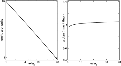
Figure 2: Normal state conductivity as a function of frequency shows a scaling behavior for $\omega_{0}<\omega<40\omega_{0}$. Left: $|\sigma(\omega)|$, the behavior is indistinguishable from the $\sigma(\omega)\sim\omega^{-0.64}$ dependence. Right: $\arctan\Im\sigma(\omega)/\Re\sigma(\omega)$, an almost constant value means that both $\Im\sigma(\omega)$ and $\Re\sigma(\omega)$ scale as $\omega^{-0.64}$.

Raman absorption measures the imaginary part of the fully renormalized particle-hole susceptibility at vanishingly small incoming momentum, weighted with Raman form factors that depend on the scattering geometry. In the $B_{1g}$ geometry the Raman form factors are $\gamma_{B_{1g}}(\mathbf{k})\propto(\cos k_{x}-\cos k_{y})$. They are the largest for fermionic momenta near $(0,\pi)$ and symmetry related points. In the $B_{2g}$ geometry, the Raman form factors are $\gamma_{B_{2g}}(\mathbf{k)}\propto\sin k_{x}\sin k_{y}$, and the Raman signal comes from around $(\pi/2,\pi/2)$ points which are close to the diagonal hot spots on the Fermi surface. For electron-doped cuprates these are the regions where we found non-Fermi liquid behavior of the fermionic self-energy.

Unlike the current vertex for conductivity, the Raman vertex is renormalized by the interaction even when $\Sigma(\omega)$ depends only on frequency. The renormalization of the $B_{1g}$ Raman vertex is not that relevant because the interaction peaked at or near $\mathbf{Q}=(\pi,\pi)$ connects regions of the Brillouin zone where the bare vertex changes sign. The ladder series pertaining to vertex renormalization is then alternate in sign and roughly renormalizes $\gamma_{B_{1g}}$ to $\gamma_{B_{1g}}/(1+A\gamma_{B_{1g}})$, where $A$ is positive. On the other hand, the $B_{2g}$ Raman vertex $\gamma_{B_{2g}}(\mathbf{k})$ does not change sign under $\mathbf{k}\rightarrow\mathbf{k}+\mathbf{Q}$. To a good approximation, we can approximate this vertex by a constant $\gamma_{B_{2g}}$. The renormalization of the Raman vertex then coincides with that of the density vertex, and like a density vertex, is then related to the self-energy by the Ward identity: the full $\gamma_{B_{2g}}^{\mathrm{full}}(\omega)=\gamma_{B_{2g}}(1+\partial_{\omega}\Sigma(\omega))$. The vertex then leads to the additional frequency dependence $\gamma_{B_{2g}}(\omega)\sim\partial_{\omega}\Sigma(\omega)$ such that $\gamma_{B_{2g}}(\omega)\propto\omega^{-\alpha}$ for $\omega<\omega_{0}$ and $\omega^{-1/4}$ for $\omega>\omega_{0}$.

Convoluting two Raman vertices with the polarization bubble we obtain, approximately

$$R_{B_{2g}}(\omega)\sim k_{y,\mathrm{max}}(\omega)\left(1+\partial_{\omega}\Sigma(\omega)\right)^{2}\frac{\omega}{\omega+\Sigma(\omega)}$$ (30)

Substituting the forms of the self-energy and $k_{y,\mathrm{max}}(\omega)\sim\omega^{\alpha}$ for $\omega<\omega_{0}$, $k_{y,\mathrm{max}}(\omega)\sim\omega^{1/4}$ for $\omega>\omega_{0}$, we find that at $T=0$, $R_{B_{2g}}(\omega)$ is flat: it is a constant at $\omega<\omega_{0}$, and slowly crosses over to the $(\omega/\omega_{0})^{-1/4}$ behavior at $\omega>\omega_{0}$.

The almost flat form of the Raman intensity at frequencies $\omega>\omega_{0}$ is consistent with the experimental data quazilbash05 . The experimental behavior at small frequencies is not flat, but according to quazilbash05 it is dominated by temperature effects which we do not consider here.

IV Pairing problem

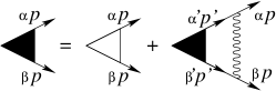
Figure 3: Diagrammatic equation on the anomalous vertex

The linearized gap equation at QCP is obtained using Eliashberg technique for collective-mode mediated pairing. Assuming that the pairing occurs in the singlet channel, we write the pairing vertex as $\Phi_{\alpha\beta}(p)=i\sigma_{\alpha\beta}^{y}\Phi(p)$ and obtain (see Fig. 3)

$$\Phi(k)=-3g^{2}\sum_{k^{\prime}}\Phi(k^{\prime})G(k^{\prime})G(-k^{\prime})\chi(k-k^{\prime})$$ (31)

where $k$ stands for a 3-component vector $(\mathbf{k},\omega)$, $\sum_{p}=T\sum_{\omega}\int d^{2}k/(2\pi)^{2}$, the Green’s functions are full: $G^{-1}(k)=G_{0}^{-1}+\Sigma(k)$, and the prefactor $-3$ comes from the convolutions of the Pauli matrices $\sigma_{\alpha^{\prime}\beta^{\prime}}^{y}\mbox{\boldmath$\sigma$}_{\alpha\alpha^{\prime}}\mbox{\boldmath$\sigma$}_{\beta\beta^{\prime}}=-3\sigma_{\alpha\beta}^{y}$. The pairing vertex $\Phi(k)$ is related to pairing gap $\Delta(k)$ as $\Phi(\mathbf{k},\omega)=\Delta(\mathbf{k},\omega)\omega/(\omega+\Sigma(\mathbf{k},\omega))$. The solution of this linearized gap equation yields both $T_{c}$ and the momentum and frequency dependence of $\Phi(\mathbf{k},\omega)$. At least close to $T_{c}$, this momentum dependence must be close to that of the true pairing gap.

As in the normal state analysis, we use the fact that bosons are slower than fermions and approximate $\chi(k-k^{\prime})$ by Fermi surface to Fermi surface interaction, i.e, put both $\mathbf{k}$ and $\mathbf{k}^{\prime}$ on the Fermi surface. Like before, we also assume that the fermionic self-energy does not depend on the momentum component transverse to the Fermi surface. We will, however, keep the momentum dependence of $\Sigma$ along the Fermi surface. We will see below that $T_{c}$ very strongly and non-analytically depends on the Fermi surface curvature $\kappa=2\beta^{2}/v_{F}$. This strong non-analytic dependence comes from the dependence on curvature of the Fermi surface to Fermi surface interaction $\chi(k-k^{\prime})$ (see below). Accordingly, we will keep the dependence on the curvature in $\chi(k-k^{\prime})$ and in the fermionic self-energy (because $\Sigma$ is an integral of $\chi(k-k^{\prime})$), but neglect it in the Jacobian for the transformation from the integration over $d^{2}k$ to the integration over $d\epsilon_{k}$, i.e., set $dk_{x}dk_{y}=(1/v_{F})d\epsilon_{k}dk_{y}$ (the notations are the same as in Fig. 1). Under these assumptions, the momentum integration transverse to the Fermi surface involves the product of two fermionic propagators and reduces to

$$\int G(p)G(-p)d\epsilon_{\mathbf{k}}=\frac{\pi}{|\omega+\Sigma(k_{y},\omega)|}$$ (32)

Substituting this into (31) and using the fact that the interaction involves momentum transfers near $Q$, we obtain

$$\Phi_{0}(k_{y},\omega_{n})=-T\sum_{\omega_{m}}\int dk_{y}^{\prime}K_{nm}(k_{y},k_{y}^{\prime})\Phi_{Q}(k_{y}^{\prime},\omega_{m}),$$ (33)

where the kernel

$$K_{nm}(k,k^{\prime})=\frac{\widetilde{\chi}(k,k^{\prime},\omega_{n}-\omega_{m})}{|\omega_{m}+\Sigma(k^{\prime},\omega_{m})|}.$$ (34)

The reduced $\widetilde{\chi}$ is defined in (19), $k_{y}$ and $k_{y}^{\prime}$ are small, and the notations $\Phi_{0}$ and $\Phi_{Q}$ imply that the pairing vertices on the right and left hand sides of (33) belong to the opposite hot spots.

Because the kernel (34) is invariant under the sign inversions of frequency and momenta, the solutions are symmetric or antisymmetric in both. A solution with $d_{x^{2}-y^{2}}$ symmetry is antisymmetric in $k_{y}$. It is also symmetric in frequency as at $T_{c}$ the largest eigenvalue of the kernel reaches unity, and from a known theorem the eigenfunction of the largest eigenvalue is symmetric in $\omega$ comm4 . As a further simplification, we consider a “antiferromagnetic” $d_{x^{2}-y^{2}}$ order parameter made out of $n=1$, $n=3$, etc. partial components of the $B_{1g}$ representation of the $D_{4h}$ group for tetragonal symmetry (i.e., $\cos k_{x}-\cos k_{y}$, $\leavevmode\nobreak\ \cos 3k_{x}-\cos 3k_{y}$, …). For the odd $n$ solutions, the pairing vertex (and the gap) change sign when the momentum is shifted by $Q$, i.e., $\Phi_{0}(k_{y},\omega_{n})=-\Phi_{Q}(k_{y},\omega_{n})$. Note that a “conventional” $\cos k_{x}-\cos k_{y}$ solution falls into this category. Using this condition and dropping the subscript we get from (33):

$$\Phi(k_{y},\omega_{n})=T\sum_{\omega_{m}}\int dk_{y}^{\prime}K_{nm}(k_{y},k_{y}^{\prime})\Phi(k_{y}^{\prime},\omega_{m}).$$ (35)

The remaining input is the polarization operator which is a part of $\tilde{\chi}$. We verified a posteriori that the dominant contribution to the pairing comes from $\omega>\omega_{0}$, where $\Pi(q,\Omega)$ scales as $\Omega^{1/2}$ and weakly depends on $q$. In principle, one should use the full, finite $T$ form of of the polarization bubble. However, the explicit temperature dependence of $\Pi$ only complicates the calculations but does not lead to any new physics. We assume without further discussion that the $T$ dependence of the polarization bubble does not alter $T_{c}$ in any substantial way and will use the same functional form $\Pi(\Omega_{m})=(g^{2}/2\pi v_{F}\beta)\sqrt{|\Omega_{m}|}$ as at $T=0$, but use discrete Matsubara frequencies at a finite $T$. For accuracy, in numerical calculations we kept the full $T$ dependence of the fermionic self-energy. We found, however, that the full form of $\Sigma(k_{y},\omega_{m},T)$ differs very little from the zero-temperature form $\Sigma(k_{y},\omega_{m})$ taken at discrete Matsubara frequencies

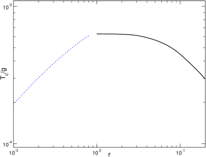
Figure 4: Pairing instability temperature $T_{c}$ in units of the coupling constant $\overline{g}$ vs. the curvature parameter $r=\bar{g}\beta^{2}/\pi v_{F}^{2}$. Solid line gives the result of the numeric solution, which requires increasingly long computational time as $r\rightarrow 0$. Dashed line is the analytic small-$r$ form $T_{c}=0.95\bar{g}r/(1+5r^{2/5})^{4}$.

We stick to $N=2$ in this section. It is convenient to measure frequency and temperature in units of $\omega_{0}$ (21) as the fermionic self-energy at $k_{y}=0$ is (23), and measure momenta $k_{y}$ in units of $q_{0}$ (20). Switching to these new units, we reproduce Eqs. (33) and (19) with

$$\widetilde{\chi}(k,k^{\prime},\Omega)=\frac{3}{2N}\frac{1}{(k-k^{\prime})^{2}+r^{2}(k^{2}+k^{\prime 2})^{2}+\sqrt{|\Omega|}}.$$ (36)

The dimensionless quantity

$$r=\bar{g}\beta^{2}/\pi v_{F}^{2}=\left(\frac{\bar{g}}{2\pi v_{F}p_{F}}\right)\kappa p_{F}$$ (37)

is proportional to both the curvature and the interaction. Both $k^{2}$ and $k^{4}$ terms in $\widetilde{\chi}(k,k^{\prime},\Omega)$ come from the original $(\mathbf{k}-\mathbf{k}^{\prime})^{2}$ term in $\chi(k-k^{\prime})$ when we use that for the two fermions on the opposite sheets of the Fermi surface $k_{x}=\beta^{2}k_{y}^{2}/v_{F}$ and $k^{\prime}_{x}=-\beta^{2}k^{\prime}_{y}{}^{2}/v_{F}$. The normalization scale $\omega_{0}$ also scales with $r$:

$$\omega_{0}\equiv\frac{\overline{g}}{4\pi}r$$ (38)

and hence the curvature is present both in the overall factor, and in the pairing susceptibility (and in the fermionic self-energy at a non-zero $k_{y}$, by virtue of the $r-$dependence of the susceptibility).

The presence of the curvature both in the overall normalization factor for $T$ and in the pairing susceptibility is what qualitatively distinguishes the $d-$wave pairing of near-nodal fermions from the pairing of antinodal fermions, which was previously studied in the context of pairing in hole-doped cuprates. In the latter case, the pairing instability temperature is finite already at zero curvature, and the effect of the curvature on $T_{c}$ is likely small (although this issue has not been analyzed in detail yet). In the present case, $T_{c}$ just vanishes without curvature, so the curvature, parameterized by $r$, plays the major role. The same $r$ also specifies momentum dependence of $\Phi(k_{y},\omega_{n})$, and, hence, of the pairing gap.

Below we will solve the gap equation separately for the cases $r\rightarrow 0$, when only the $r-$dependence of the overall factor matters, and for finite $r$, when the $rk^{4}$ term in the pairing susceptibility has to be taken into consideration. We will see that the $r-$dependence in the denominator of (36) becomes relevant already at very small $r$, and for $r\sim 0.1$, relevant to the cuprates (see below), the actual $T_{c}$ is much smaller than the one obtained by keeping the curvature only in the overall factor.

IV.1 Solution at $r\rightarrow 0$ (vanishing curvature)

When we put $r=0$ in the susceptibility (36), the gap equation (35) simplifies considerably. First, the fermionic self-energy loses its dependence on $k_{y}$ and becomes

$$\Sigma(k_{y},\omega_{m})=\Sigma(\omega_{m})=\mathop{\mathrm{sgn}}\nolimits\omega_{m}\frac{3}{4}\pi T\sum_{|\Omega_{n}|<|\omega_{m}|}|\Omega_{n}|^{-1/4}.$$ (39)

We used the full summation in the numerical calculations below, but this is actually not even necessary – we found that for $T=T_{c}$, the functional form of the self-energy is close to the zero-temperature expression $\mathop{\mathrm{sgn}}\nolimits\omega_{m}|\omega_{m}|^{3/4}$ for all Matsubara frequencies.

Second, without the $r$ term in $\tilde{\chi}$, momentum dependence of the kernel (34) is of a convolution type: $K(k_{y},k_{y}^{\prime})=K(k_{y}-k_{y}^{\prime})$. This implies that Eq. (35) is local in real space coordinate $y$ conjugate to the momentum $k_{y}$, as can be easily seen by taking reverse Fourier transform in $k_{y}$. The kernel $K(k_{y}-k_{y}^{\prime})$ is not double integrable:

$$\int_{-\infty}^{\infty}\left|K(k,k^{\prime})\right|dkdk^{\prime}=\infty$$ (40)

and so the integral equation in $k_{y}$ is non-Fredholmian, which means it does not have a countable spectrum with integrable eigenfunctions. However, the kernel is still uniformly finite

$$\int_{-\infty}^{\infty}\left|K(k,k^{\prime})\right|dk=\int_{-\infty}^{\infty}\left|K(k,k^{\prime})\right|dk^{\prime}<\infty,$$ (41)

and thus may have finite solutions. Two such solutions can be easily guessed: a symmetric one: $\Phi(k_{y},\omega_{n})=\Phi(\omega_{n})$ and an antisymmetric one: $\Phi(k_{y},\omega_{n})=k_{y}\Phi(\omega_{n})$. As functions of real space coordinate $y$ these two solutions correspond to $\delta(y)\Phi(\omega_{n})$ and $-(d\delta(y)/dy)\Phi(\omega_{n})$, respectively, where $\delta(y)$ is a delta function. The $d-$wave solution we are interested is the one antisymmetric in $k_{y}$. In both cases, integrating explicitly over momentum and substituting the result for the susceptibility, we obtain one-dimensional integral equation for $\Phi(\omega_{n})$:

$$\Phi(\omega_{n})=\frac{3}{4}\pi T$$

$$\times\sum_{\omega_{m}}\frac{\Phi(\omega_{m})}{|\omega_{n}-\omega_{m}|^{1/4}\left(|\omega_{m}|+\frac{3}{4}\pi T\sum_{|\Omega_{n}|<|\omega_{m}|}|\Omega_{n}|^{-1/4}\right)}$$ (42)

Approximating the self-energy by the $\omega^{3/4}$ form simplifies (42) to

$$\Phi(\omega_{n})=\frac{3}{4}\pi T\sum_{\omega_{m}}\frac{\Phi(\omega_{m})}{|\omega_{m}+\Sigma(\omega_{m})||\omega_{n}-\omega_{m}|^{1/4}}.$$ (43)

This equation falls into a generic class of local Eliashberg-type gap equations with the effective local pairing interaction $\chi_{l}(\omega)\propto\omega^{-\gamma}$ for which the fermionic self-energy scales as $\omega^{1-\gamma}$ (unpubl , see also Appendix D). Eq. (43) corresponds to $\gamma=1/4$.

Note that: (i) the gap equation is fully universal and parameter-free (we recall that $T$ is in units of $\omega_{0}$), and (ii) that self-energy term is not small and cannot be neglected. At small $\omega_{m}=\pi T(2m+1)<1$, the kernel of the gap equation scales as $1/\omega$. This power is a combination of $1/\omega^{1/4}$ from the effective local pairing interaction and $\omega^{3/4}$ from the fermionic self-energy. At $\omega_{m}>1$, the kernel decays as $1/\omega^{5/4}$, i.e., faster than $1/\omega$, and the frequency sum converges even without $\Phi(\omega_{m})$. Ref. unpubl argued that, this gap equation has a non-zero solution at $T=O(1)$.

We solved this equation numerically (the details are presented in Appendix D) and found, in actual units

$$T_{c}(r\rightarrow 0)\approx 6\omega_{0}\equiv 6\frac{\overline{g}}{4\pi}r,$$ (44)

The scaling with the upper cutoff of the quantum-critical behavior ($\omega_{0}$ in our case) is the same as in hole-doped materials (where the pairing involves predominantly antinodal fermions), however, we emphasize that in our case the scale $\omega_{0}$ is by itself proportional to the Fermi surface curvature, while the corresponding scale for antinodal pairing remains finite in the absence of the curvature.

Note in passing that the prefactor is much larger in our case than for antinodal pairing, where $T\approx 0.2$ in units of the upper cutoff of the quantum-critical behavior  abanov03 .

IV.2 Solution at finite $r$

IV.2.1 Numerical solution

Although $T_{c}$ given by (44) is finite, the solution of the gap equation without the $r^{2}k_{y}^{4}$ term in the susceptibility is unphysical since the pairing gap continuously increases with $k_{y}$: $\Phi(k_{y},\omega_{n})\propto k_{y}$. This behavior reflects translational invariance of the pairing potential (or, in mathematical language, the non-Fredholmian property of the integral equation). When the $r^{2}k^{4}$ term is kept in $\widetilde{\chi}(k_{y},k_{y}^{\prime},\omega)$, Eq. (35) becomes Fredholmian, its solutions integrable, and the gap vanishes at large $k_{y}$. A numerical solution of the gap equation can then be obtained by standard technique. We solved Eq. (35) numerically in the quadrant $\omega,k>0$, searching for a solution $\Phi_{n}(k)$ that is symmetric in $\omega_{n}$ and antisymmetric in $k$. The semiinfinite integral over $k$ was mapped onto the interval $[0,1)$ using the transformation $x=(1-k)/k$, and then integration was approximated by Gauss-Legendre quadrature: $\int_{0}^{1}f(x)dx=\sum_{i}f(x_{i})w_{i}$, where $x_{i}$ and $w_{i}$are the abscissas and weights of the quadrature. This procedure is called the Nystrom method nr . The integral equation then reduces to an (infinite in the Matsubara frequency index $n$) set of algebraic equations:

$$\Phi_{ni} = \sum_{m\geq 0,j}(K_{nimj}+K_{ni,-m-1,j}$$ (45)

$$-K_{nim,-j}-K_{ni,-m-1,-j})\Phi_{mj},$$

This set was truncated and solved by standard LAPACK routines. This procedure gives good approximation to the largest eigenvalues of the kernel, and for the critical temperature we need just the largest one.

We found that the effect of the curvature on $T_{c}$ is very strong: above $r>0.001$, the actual $T_{c}$ rapidly becomes much smaller than (44). We plot $T_{c}(r)$ in Fig. 4 in units of $\overline{g}/4\pi$. We see that over a wide range $0.01<r<0.1$, $T_{c}\approx 0.0005\bar{g}$ forms a plateau and weakly depends on $r$. Using the same $\overline{g}\sim 1.6$eV and the $t$-$t^{\prime}$ dispersion as in hole-doped materials abanov02 but with positive chemical potential to reproduce the Fermi surface in Fig. 1, we obtained $r\sim 0.08$, which is within the region where $T_{c}$ is almost constant, and $T_{c}\sim 10$K. For hole-doped cuprates, for the same parameters, the onset of the pairing was earlier estimated at $T_{c}\sim 0.01\overline{g}\sim 200K$ abanov03 , although this number may also be reduced by the curvature of the Fermi surface.

The theoretical value of $T_{c}\sim 10$K at a magnetic QCP in electron-doped cuprates is in reasonable agreement with the experiment el-pd ; quazilbash05 ; zimmers05 . Maximum $T_{c}$ in Nd_2-xCe_xCuO₄ and Pr_2-xCe_xCuO₄ is about $20-25$K, but, according to  zimmers05 , $T_{c}$ initially increases once the system becomes magnetically ordered. In any event, even $50\%$ agreement is quite reasonable given the number of approximations in our theoretical analysis. Note that if we used Eq. (44) for $T_{c}$ instead of the correct result, we would have obtained a very large $T_{c}\sim 600$K for the same parameters. This shows that the Fermi surface curvature truly plays a major role when the pairing involves near-nodal fermions.

The reduction of $T_{c}$ in electron-doped cuprates, compared to hole-doped cuprates with the same interaction strength was also obtained in FLEX calculations manske00 , although the reported difference was less drastic than in our analysis.

In Fig 5 we present the result for the momentum dependence of the pairing vertex at various frequencies. We see that the pairing gap is a non-monotonic function of $k_{y}$: it initially increases with $k_{y}$, but then passes through a maximum and decreases at larger $k_{y}$. This result agrees with earlier BCS calculations yakovenko04 , but we emphasize that our gap equation is of non-BCS form. We also emphasize that the position of the maximum in $\Phi(k_{y},\omega)$ is disconnected from the location of the hot spots which in our QCP analysis are exactly along the Brillouin zone diagonals, i.e., at $k_{y}=0$.

IV.2.2 Toy model

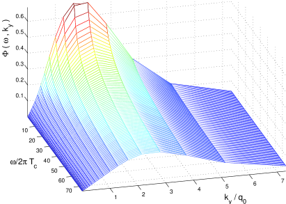
Figure 5: The pairing vertex $\Phi(k_{y},\omega_{n})$ for $r=0.05$ vs $\omega_{n}/(2\pi T_{c})$ and $k_{y}/q_{0}$ ($q_{0}$ is defined in the text). Observe that $\Phi(k_{y},\omega_{n})$ is non-monotonic in $k_{y}$.

The large discrepancy between $T_{c}(r)$ and (44) can also be understood analytically, by expanding $T_{c}$ in $r$ beyond the $O(r)$ term. This expansion is rather non-trivial as one has to expand around a solution which diverges at large $k_{y}$, and the divergence must be cut by the corrections which then obviously are not small at large $k_{y}$. Since this effect is unrelated to the summation over Matsubara frequencies, which at $T_{c}$ is confined to first few $m$, we can simplify the model by dropping the frequency summation, and instead of (35), analyze the approximate form of the gap equation

$$\Phi(k)=\frac{3}{4\pi}\int\frac{\Phi(k^{\prime})dk^{\prime}}{(k-k^{\prime})^{2}+r^{2}(k^{2}+k^{\prime 2})^{2}+x^{2}},$$ (46)

In (46) we set $x^{4}=a(T/\omega_{0})$ with $a\approx 3^{3}/2^{9}$ to match Eq. (44) at vanishing $r$. To shorten notations, we dropped the subscript $y$ from $k_{y}$.

Equation (46) can be analyzed analytically. Our goal is to understand why $T_{c}$ drops by two orders of magnitude compared to $6\omega_{0}$ already at relatively small $r\sim 0.1$.

We search for the solution of (46) in the form

$$\Phi(k)=\Phi_{0}(k)+\delta\Phi(k),$$ (47)

where $\Phi_{0}(k)=k$ is the unphysical solution at $r\to 0$ found in Subsection IV.1, and consider $\delta\Phi(k)$ as perturbation. Substituting into (46) and expanding in $\delta\Phi$, we obtain

$$\delta\Phi(k) - \frac{3}{4\pi}\int\frac{\delta\Phi(k^{\prime})dk^{\prime}}{(k-k^{\prime})^{2}+x_{0}^{2}}=\frac{3k}{4\sqrt{x^{2}+4r^{2}k^{4}}}-k$$ (48)

$$\approx \left(\frac{3}{4x}-1\right)k-\frac{3r^{2}k^{5}}{2x_{0}^{3}}$$

where $x_{0}=3/4$, and we dropped the regular $O(r)$ terms from the integral

$$\int\frac{\Phi_{0}(k^{\prime})dk^{\prime}}{(k-k^{\prime})^{2}+r^{2}(k^{2}+k^{\prime 2})^{2}+x^{2}}$$ (49)

and the higher-order terms in the expansion of the square-root in (48). We will see below that relevant $k$ are of order $r^{-2/5}$ and $3/4x-1$ is of order $r^{2/5}$, so that $r^{2}k^{4}\sim r^{2/5}$, which justifies both the expansion of the square-root in (48) and dropping the regular $O(r)$ terms.

We search for the solution of (48) in the form

$$\delta\Phi(k)=r^{2}\left(Ak^{3}+Bk^{5}\right),\qquad|k|<k_{\mathrm{m}},$$ (50)

where $k_{\mathrm{m}}$ is a cutoff that has to be found from an auxiliary condition that the solution (47) with $\delta\Phi(k)$ in the form of (50) is unique. Substituting (50) into (48) and using

$$\int_{-k_{\mathrm{m}}}^{k_{\mathrm{m}}}\frac{k^{\prime 3}dk^{\prime}}{(k-k^{\prime})^{2}+x_{0}^{2}} \approx k^{3}\frac{\pi}{x_{0}}+6kk_{\mathrm{m}}$$ (51)

$$\int_{-k_{\mathrm{m}}}^{k_{\mathrm{m}}}\frac{k^{\prime 5}dk^{\prime}}{(k-k^{\prime})^{2}+x_{0}^{2}} \approx k^{5}\frac{\pi}{x_{0}}+20k^{3}k_{\mathrm{m}}+\frac{10}{3}kk_{\mathrm{m}}^{3}$$ (52)

we obtain

$$\frac{3}{4\pi}\int\frac{\delta\Phi(k^{\prime})dk^{\prime}}{(k-k^{\prime})^{2}+x_{0}^{2}}\approx$$ (53)

$$\frac{3r^{2}}{4\pi}\left[k(6k_{\mathrm{m}}A+\frac{10}{3}k_{\mathrm{m}}^{3}B)+k^{3}(\frac{\pi}{x_{0}}A+20k_{\mathrm{m}}B)+k^{5}\frac{\pi}{x_{0}}B\right].$$

Substituting this into (48) and equating the prefactors for $k$, $k^{3}$ and $k^{5}$ terms in (48), we obtain the set of equations

$$\left(\frac{3}{4x}-1\right)B = \frac{3}{2x_{0}^{3}}$$ (54)

$$\left(\frac{3}{4x}-1\right)A = -\frac{15}{\pi}k_{\mathrm{m}}B$$ (55)

$$-\frac{r^{2}}{2\pi}(9k_{\mathrm{m}}A+5k_{\mathrm{m}}^{3}B) = \left(\frac{3}{4x}-1\right)$$ (56)

Solving the set, we obtain

$$\frac{(3/4x-1)^{5}}{r^{2}}=\frac{80u^{2}}{9\pi}\left(\frac{27}{\pi}-u\right),$$ (57)

where $u=k_{\mathrm{m}}(3/4x-1)$. A unique solution of this equation exists when $u=18/\pi$ and

$$\left(\frac{3}{4x}-1\right)\approx r^{2/5}\left(\frac{320*81}{\pi^{4}}\right)^{1/5}\approx 3r^{2/5}$$ (58)

Using the definition of $x$ we then obtain

$$T_{c}\approx 6\frac{\bar{g}}{4\pi}\frac{r}{(1+3r^{2/5})^{4}}$$ (59)

This formula is formally valid at small $r$, but it works surprisingly well for all $r<1$ as evidenced by the comparison of (59) with the numerical solution of (48). We compare analytic and numerical results in Fig. 6, 7.

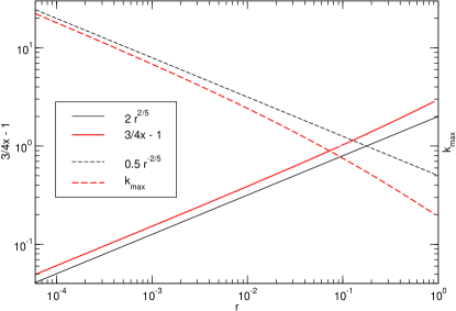
Figure 6: Scaling of the “critical temperature” $x(r)$ (solid lines) and the position of the maximum $k_{\textrm{m}}(r)$ (dashed lines) with the parameter $r$ in the kernel (36) of the one-dimensional “toy model”. Numerical solution (red curves) closely follow the scaling laws obtained analytically (black straight lines): $3/4x-1\approx 2r^{2/5}$, and $k_{\mathrm{m}}\sim r^{-2/5}$.

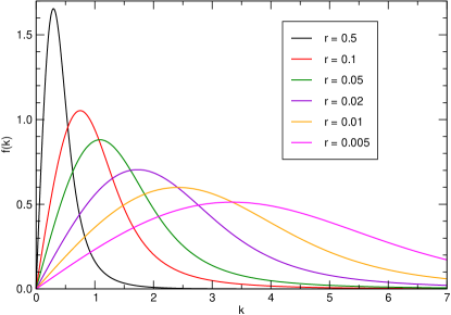
Figure 7: Solutions $f(k)$ of the one-dimensional “toy model” for several values of the parameter $r$ ($r$ decreases for the curves from left to right). Dependence of the position of the maximum $k_{\mathrm{m}}(r)$ is plotted in Fig. 6.

Eq. (59) shows that $T_{c}$ does indeed drop quite substantially, compared to the asymptotic linear behavior (44): at $r\sim 0.1$, $(1+3r^{2/5})^{4}\approx 23$. Furthermore, $T_{c}$ given by (59) is rather flat at intermediate $r\sim 0.04-0.5$ where $T_{c}\sim 0.02{\bar{g}}$. This is consistent with the numerical solution of (48). The flat behavior in a wide range of $r$ reproduces what we have found numerically for the full gap equation (with the full frequency summation).

We also see from (55) that $A\sim r^{-6/5}$, $B\sim r^{-2/5}$, and the cutoff $k_{\mathrm{m}}$ diverges as

$$k_{\mathrm{m}}=u/\left(\frac{3}{4x}-1\right)\sim r^{-2/5}$$ (60)

Substituting $k_{\mathrm{m}}$ and $A$ and $B$ into (50), we obtain

$$\delta\Phi(k)\sim\Phi_{0}(k)\left(\left(k/k_{\mathrm{m}}\right)^{2}+a\left(k/k_{\mathrm{m}}\right)^{4}\right),\qquad a=O(1)$$ (61)

We see that at $k\sim k_{\mathrm{m}}$, the corrections to zero-order solution become of order 1. A perturbation theory does not allow one to go beyond this scale (i.e., to analyze $\delta\Phi(k)$ for $k>k_{\mathrm{m}}$), but it is reasonable to assume that above $k_{\mathrm{m}}$, $\Phi(k)=\Phi_{0}(k)+\delta\Phi(k)$ begins decreasing. The numerical solution of (48) confirms this (see Fig. 7). We see from Fig. 7 that the gap in the toy model is a non-monotonic function of $k_{y}$: it is linear at small $k_{y}$, passes through a maximum at $k_{y}\sim k_{\mathrm{m}}$, and then falls off. This behavior is again fully consistent with what we have obtained numerically for the full gap equation.

Returning to the actual, unrescaled momenta $k_{y}$, we obtain, using the definition of $r$, that the maximum of the gap is located at

$$k_{\mathrm{m}}=\frac{\overline{g}}{\pi v_{F}}k_{\mathrm{m}}\sim\frac{\overline{g}}{v_{F}}r^{-2/5}\sim k_{F}r^{3/5}\left(\frac{\beta_{0}}{\beta}\right)^{2}$$ (62)

where $\beta_{0}^{2}=v_{F}/k_{F}$. For $\beta\sim\beta_{0}$, and $r\ll 1$, $k_{\mathrm{m}}$ is much less than $k_{F}$, i.e., the $d-$wave gap is confined to a near vicinity of the zone diagonal.

We fitted the actual $T_{c}$ for the full model by the functional form of Eq. (59), using the prefactor for the $r^{2/5}$ term as the adjusting parameter. We found that the numerical data are reproduced reasonably well if we set this prefactor to $5$ (instead of $3$ in Eq. (59)). We show the fit in Fig. 4.

IV.3 Away from the QCP

At deviations from the QCP towards larger dopings, i.e., into paramagnetic phase, $T_{c}$ decreases and eventually disappears. The value of $k_{\mathrm{m}}$, however, does not track the decrease of $T_{c}$, i.e., the $d-$wave gap extends over a finite momentum range along the FS even in the overdoped materials. At deviations into antiferromagnetic phase, the FS evolves into hole and electron pockets, and the locations of $k_{\mathrm{m}}$ gradually approach the locations of the hot spots.

Our results for $T_{c}$ and the gap survive even when the magnetic correlation length $\xi$ remains finite at the doping where $2k_{F}=Q$ and the Fermi surface has the form shown in Fig. 1. In this situation, the antiferromagnetic QCP shifts to lower dopings, when the hot spots are already away from the Brillouin zone diagonals. We found that the modifications of our results are small as long as $T_{c}>J\xi^{-2}$ where $J\sim v_{F}^{2}/{\bar{g}}$ is of the order of the the exchange interaction.

V Summary

We considered the normal state properties and pairing near a $2k_{F}$ antiferromagnetic QCP and applied the results to electron-doped cuprates at optimal doping. We found that the breakdown of the Fermi-liquid description at QCP leads to peculiar frequency dependences of the conductivity and the $B_{2g}$ Raman response. We found that $T_{c}$ remains finite at the QCP. The pairing gap at QCP has $d_{x^{2}-y^{2}}$ symmetry, but is highly anisotropic and confined to momenta near the zone diagonals. The value of $T_{c}$ is about $10$K for the same spin-fermion coupling as for hole-doped cuprates, where the pairing predominantly involves antinodal fermions. The strong reduction of $T_{c}$ compared to hole-doped case is due to the fact that for the $d-$wave pairing of near-nodal fermions, the curvature of the Fermi surface plays a major role.

We acknowledge useful discussions with G. Blumberg, D. Drew, I. Eremin, R. Greene, C. Homes, D. Manske, A. Millis, B.S. Mityagin, M. Norman, S.P. Novikov, M. M. Qazilbash, and V. Yakovenko. The research is supported by Condensed Matter Theory Center at UMD (P.K, A.C) and by NSF DMR 0240238 (A.C.).

Appendix A Transformation of the polarization operator when hot spots merge

In this Appendix we detail the transformation of the polarization operator with the shift in the position of the hot spots along the Fermi surface. In hole-doped materials the spots with the strong electron interaction are close to the $(0,\pi)$ and symmetry-related points on the Fermi surface in the notations of Fig. 1. With doping and expansion of the Fermi surface its boundary crosses the antiferromagnetic Brillouin zone at points that become closer to each other and to the zone diagonal until in electron-doped cuprates they merge pairwise at the doping level when the Fermi surface just touches the antiferromagnetic Brillouin zone at $(\pi/2,\pi/2)$ (this situation is shown in Fig. 1). In hole-doped materials it sufficed to take linear approximation of electron dispersion near the hot spots: $\epsilon_{\mathbf{k}}=\mathbf{v}_{F}\mathbf{k}$. The polarization operator of non-interacting fermions then had the Landau damping form

$$\Pi(\mathbf{q},\Omega)=g^{2}|\Omega|/4\pi v_{x}v_{y},$$ (63)

where $g$ is the coupling, and $\mathbf{v}_{F}=(v_{x},v_{y})$ abanov03 . In the situation depicted in Fig. 1 one has to keep second order terms in $\epsilon_{\mathbf{k}}$ (8), and the bare polarization operator has the form (10). Here we show how to go from (63) to (10) with continuous change in the electron spectrum. For later use we will carry out slightly more general calculation keeping fermionic self-energy that depends only on frequency. Consider a spectrum that has both linear term in transverse momentum and curvature:

$$\epsilon_{\mathbf{k}} = v_{x}k_{x}+v_{y}k_{y}+\beta^{2}k_{y}^{2},$$ (64)

$$\epsilon_{\mathbf{k}+\mathbf{Q}} = -v_{x}k_{x}+v_{y}k_{y}+\beta^{2}k_{y}^{2}.$$ (65)

The case $\beta=0$ gives dispersion around well-separated hot-spots of hole-doped materials, and in the case $v_{y}=0$ we revert to (8). To alleviate integration in $\mathbf{k}$ we note that the following equality holds

$$\epsilon_{\mathbf{k}}+\epsilon_{\mathbf{k}+\mathbf{q}+\mathbf{Q}}=\widetilde{E}_{\mathbf{q}}+y^{2},$$ (66)

where

$$\widetilde{E}_{\mathbf{q}}=-v_{x}q_{x}+\frac{\beta^{2}q_{y}^{2}}{2}-\frac{v_{y}^{2}}{2\beta^{2}}$$ (67)

differs from $E_{\mathbf{q}}$ (11) by $-v_{y}^{2}/2\beta^{2}$, and

$$y=\sqrt{2}\beta\left(k_{y}+\frac{q_{y}}{2}+\frac{v_{y}}{2\beta^{2}}\right)$$ (68)

is a convenient dummy variable in the integration instead of $k_{y}$. The Jacobian of the substitution $\mathbf{k}\rightarrow(\epsilon_{\mathbf{k}},y)$ is

$$\left|\frac{\partial(\epsilon_{\mathbf{k}},y)}{\partial(k_{x},k_{y})}\right|=\sqrt{2}v_{x}\beta.$$ (69)

Momentum integration in (6) then gives

$$\Pi(\mathbf{q},\Omega)=2g^{2}\int\frac{d\omega d^{2}\mathbf{k}}{(2\pi)^{3}}G\left(\mathbf{k},\omega-\textstyle\frac{\Omega}{2}\right)G\left(\mathbf{k}+\mathbf{q},\omega+\textstyle\frac{\Omega}{2}\right)$$

$$=\frac{ig^{2}}{4\pi\sqrt{2}v_{x}\beta}\int\frac{\mathop{\mathrm{sgn}}\nolimits\left(\omega+\frac{|\Omega|}{2}\right)+\mathop{\mathrm{sgn}}\nolimits\left(\omega-\frac{|\Omega|}{2}\right)}{\sqrt{\widetilde{E}_{\mathbf{q}}-i\left(\widetilde{\Sigma}_{\omega+\frac{|\Omega|}{2}}+\widetilde{\Sigma}_{\omega-\frac{|\Omega|}{2}}\right)}}d\omega,$$ (70)

where $\widetilde{\Sigma}_{\omega}=\omega+\Sigma(\omega)$. Simplifying frequency integration from the antisymmetric integrand

$$\Pi(\mathbf{q},\Omega)=\frac{g^{2}}{\sqrt{2}\pi v_{x}\beta}\int\limits_{|\Omega|/2}^{\infty}\Im\frac{d\omega}{\sqrt{\widetilde{E}_{\mathbf{q}}+i\left(\widetilde{\Sigma}_{\omega+\frac{|\Omega|}{2}}+\widetilde{\Sigma}_{\omega-\frac{|\Omega|}{2}}\right)}},$$ (71)

or, with the substitute $\omega\rightarrow\omega+|\Omega|/2$,

$$\Pi(\mathbf{q},\Omega)=-\frac{g^{2}}{2\pi v_{x}\beta}\int_{0}^{\infty}\frac{\sqrt{\sqrt{\widetilde{E}_{\mathbf{q}}^{2}+(\widetilde{\Sigma}_{\omega}+\widetilde{\Sigma}_{\omega+|\Omega|})^{2}}-\widetilde{E}_{\mathbf{q}}}}{\sqrt{\widetilde{E}_{\mathbf{q}}^{2}+(\widetilde{\Sigma}_{\omega}+\widetilde{\Sigma}_{\omega+|\Omega|})^{2}}}d\omega.$$ (72)

When $\Sigma(\omega)=0$ the integral above can be taken exactly and gives

$$\Pi(\mathbf{q},\Omega)=\frac{g^{2}}{2\pi v_{x}\beta}\sqrt{\sqrt{\Omega^{2}+\widetilde{E}_{\mathbf{q}}^{2}}+\widetilde{E}_{\mathbf{q}}},$$ (73)

which coincides with (10) when $v_{y}=0$ and so $\widetilde{E}_{\mathbf{q}}=E_{\mathbf{q}}$. In the opposite limit $\beta\rightarrow 0$, $\widetilde{E}_{\mathbf{q}}\rightarrow-v_{y}^{2}/2\beta^{2}$ and, expanding (73) up to first order in $|\Omega|/\widetilde{E}_{\mathbf{q}}$ gives

$$\Pi(\mathbf{q},\Omega)=g^{2}|\Omega|/2\pi v_{x}v_{y},$$ (74)

i.e. exactly twice the expression (63), accounting for the pair of hot spots that emerge.

Appendix B Self-energy at $T=0$

In this Appendix we find self-consistent fermionic self-energy $\Sigma(\omega)$ at low frequencies as explained in Section III.2. Following the derivation that leads to Eq. (10) it can be shown that the polarization operator of interacting fermions that have self-energy $\Sigma(\omega)$ is

$$\Pi(\mathbf{q},\Omega)=-\frac{g^{2}}{2\pi v_{F}\beta}\int_{0}^{\infty}\frac{\sqrt{\sqrt{E_{\mathbf{q}}^{2}+(\widetilde{\Sigma}_{\omega}+\widetilde{\Sigma}_{\omega+|\Omega|})^{2}}-E_{\mathbf{q}}}}{\sqrt{E_{\mathbf{q}}^{2}+(\widetilde{\Sigma}_{\omega}+\widetilde{\Sigma}_{\omega+|\Omega|})^{2}}}d\omega.$$ (75)

where $\widetilde{\Sigma}_{\omega}=\omega+\Sigma(\omega)$. It is easy to see that in the case $\Sigma(\omega)=0$ the integral above can be taken exactly and gives (10). Note that we subtract divergent high-energy contribution

$$\Pi_{0}(0,0)=-\frac{g^{2}}{2\pi v_{F}\beta}\int_{0}^{\infty}\frac{d\omega}{\sqrt{2\widetilde{\Sigma}_{\omega}}}$$ (76)

because it is already included in the theory as the $\xi^{-2}$ “mass” term in the bare susceptibility (2).

The above expression for $\Pi$ when substituted as the bosonic self-energy in the bosonic propagator (7) in Eq. (16) yields a self-consistent equation on $\Sigma$. We will seek a solution to this equation in the form of a power law: $\widetilde{\Sigma}_{\omega}=\sigma\omega^{\gamma}$, where $\sigma$ is a constant. Using the substitutions $\Omega=|\omega|t$ so that $\widetilde{\Sigma}_{\Omega}=\widetilde{\Sigma}_{\omega}t^{\gamma}$, and $\omega^{\prime}=|\omega|ts$, where $\omega^{\prime}$ is the dummy variable in $\Pi$, so that $\widetilde{\Sigma}_{\omega^{\prime}}+\widetilde{\Sigma}_{\omega^{\prime}+\Omega}=\widetilde{\Sigma}_{\Omega}(s^{\gamma}+(s+1)^{\gamma})$, and $q=(2\widetilde{\Sigma}_{\Omega})^{1/2}v/\beta$, we arrive at a condition on the exponent $\gamma$:

$$\frac{\pi N}{3\sqrt{2}}=-\frac{1}{\gamma}\int_{0}^{\infty}f(v;\gamma)dv,$$ (77)

where

$$\frac{1}{f(v;\gamma)} = \int_{0}^{\infty}\biggl{(}\frac{\sqrt{\sqrt{v^{4}+(s^{\gamma}+(s+1)^{\gamma})^{2}}+v^{2}}}{\sqrt{v^{4}+(s^{\gamma}+(s+1)^{\gamma})^{2}}}$$

$$+ \frac{\sqrt{\sqrt{9v^{4}+(s^{\gamma}+(s+1)^{\gamma})^{2}}-3v^{2}}}{\sqrt{9v^{4}+(s^{\gamma}+(s+1)^{\gamma})^{2}}}-\frac{2}{\sqrt{2s^{\gamma}}}\biggr{)}ds.$$

The right-hand side of Eq. (77) is a continuous function of $\gamma$ in $\frac{2}{3}<\gamma<1$. It monotonically grows from zero at $\gamma=\frac{2}{3}$ and crosses the constant $\pi N/3\sqrt{2}$ at $\gamma\approx 0.85$ (see Fig. 8). Recalling that $\alpha$ used in the main body of the paper is $\alpha=1-\gamma$, we get $\alpha\approx 0.15$ as was ascertained.

The calculation of the right-hand side of Eq. (77) takes some care. Integral (B) diverges at the upper limit when $\gamma\rightarrow\frac{2}{3}$. Expanding in large $s$ gives for the residual of (B)

$$\int_{s_{\mathrm{m}}}^{\infty}(\ldots)ds\approx\frac{1}{\sqrt{2}}\left(\frac{v^{2}s_{\mathrm{m}}^{1-3\gamma/2}}{2(1-3\gamma/2)}-s_{\mathrm{m}}^{-\gamma/2}+\ldots\right),$$ (79)

whence $\int f(v;\gamma)dv\sim\sqrt{1-3\gamma/2}$ for $\gamma$ close to $\frac{2}{3}$. In the opposite limit $\gamma\rightarrow 1$ it is the integral over $v$ in (77) that diverges at the upper limit. At large $v$ the scaling substitution $s=v^{2/\gamma}z$ into (B) separates an integral over $z$:

$$\frac{1}{f(v;\gamma)}\approx C(\gamma)v^{\frac{2}{\gamma}-1},$$ (80)

so the residual of the integral over $v$ in (77)

$$\int_{v_{\mathrm{m}}}^{\infty}f(v;\gamma)dv\approx-\frac{v_{\mathrm{m}}^{\frac{2}{\gamma}-2}}{(\frac{2}{\gamma}-2)C(\gamma)}$$ (81)

diverges as $\sim(1-\gamma)^{-1}$. The auxiliary integral

$$C(\gamma) = \int_{0}^{\infty}\biggl{(}\frac{\sqrt{\sqrt{1+(2z^{\gamma})^{2}}+1}}{\sqrt{1+(2z^{\gamma})^{2}}}$$ (82)

$$+ \frac{\sqrt{\sqrt{9+(2z^{\gamma})^{2}}-3}}{\sqrt{9+(2z^{\gamma})^{2}}}-\frac{2}{\sqrt{2z^{\gamma}}}\biggr{)}dz.$$

It is negative in the interval $\frac{2}{3}<\gamma<1$ and diverges when $\gamma$ approaches $\frac{2}{3}$. When $\gamma=1$ the integral can be taken analytically: $C(1)=-\sqrt{6}$. To produce Fig. 8 we combined the numerical integration upto the finite cutoff with the analytical residuals found above.

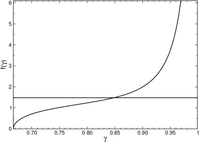
Figure 8: Graphical solution to Eq. (77). Straight line and the curve represent the left and right-hand side of Eq. (77). Crossing is at about $\gamma\approx 0.85$, or $\alpha=1-\gamma\approx 0.15$.

Appendix C Choice of the cutoff for the conductivity

In this Appendix we substantiate our claim that the frequency dependence of the conductivity does not rely on how the integration over transverse momenta in (28) is estimated. To evaluate the integral over $k_{y}$ we assumed that $\Sigma(\epsilon,k_{y})$ stays almost constant and equal to $\Sigma(\epsilon)$ for $|k_{y}|<k_{y,\mathrm{max}}$ and then falls off rapidly. Crudely we may just replace $\int dk_{y}$ with $k_{y,\mathrm{max}}$. However, since $k_{y,\mathrm{max}}\propto\omega^{\gamma}$ depends on frequency, it is not clear whether we should choose the external $\omega$ or the internal frequency $\epsilon$ for the cutoff. Choosing the first one yields

$$\sigma(i\omega)\propto\omega^{\gamma-1}\int_{0}^{\omega}\frac{d\epsilon}{\omega+\Sigma(\omega-\epsilon)+\Sigma(\epsilon)}.$$ (83)

On the other hand, if we simply integrate over $k_{y}$ in (28) with $\Sigma(\epsilon,k_{y})=\Sigma(\epsilon)$ for $|k_{y}|<k_{y,\mathrm{max}}$, the result is

$$\sigma(i\omega) \propto 2\int_{0}^{\omega/2}\biggl{(}\frac{\epsilon^{\gamma}}{\omega+\Sigma(\omega-\epsilon)+\Sigma(\epsilon)}$$ (84)

$$+\frac{(\omega-\epsilon)^{\gamma}-\epsilon^{\gamma}}{\omega+\Sigma(\omega-\epsilon)}\biggr{)}d\epsilon.$$

Intuitively, the choice of the cutoff of the momentum integration should not alter the frequency dependence of the conductivity since the internal $\epsilon$ stays of order of the external $\omega$ anyway. And indeed we found that all three estimates lead to the same pseudo-scaling of $\sigma(\omega)$ in the range $\omega_{0}<\omega<40\omega_{0}$. The choice of the cutoff alters only the irrelevant preexponent shared by both $\Re\sigma$ and $\Im\sigma$.

The fact that $\Re\sigma$ and $\Im\sigma$ scale together with $|\sigma(\omega)|$ can be seen from $\arctan(\Im\sigma/\Re\sigma)$ staying almost constant over the range $\omega_{0}<\omega<40\omega_{0}$ (see Fig. 2, right panel). The value of the constant $\varphi=\arctan(\Im\sigma/\Re\sigma)$ itself changes with the Wick transition from Matsubara to real frequencies. In particular, $\varphi$ depends on whether the Matsubara or real frequency enters the momentum cutoff $k_{y,\mathrm{max}}(\omega)$. We argue that it is logical to cut off the momentum integration on Matsubara frequencies since the subsequent frequency integration is done over Matsubara frequencies as well. With this choice the constant $\varphi\approx 1$ (see Fig. 2, right panel).

Appendix D Eliashberg local pairing

In this Appendix we describe the numerical solution of the pairing problem (42) for a general power-law local interaction. The results of this Section were used for $T_{c}$ of (43).

The general interaction is (the frequencies and the temperature are measured in suitable units which we put unity)

$$\chi(\Omega_{n})=\pi(1-\gamma)|\Omega_{n}|^{-\gamma}.$$ (85)

Fermionic self-energy $\Sigma(\omega_{n})$ corresponding to (85) is given by

$$\Sigma(\omega_{n})=T\sum_{\omega_{m}}\mathop{\mathrm{sgn}}\nolimits\omega_{m}\chi(\omega_{n}-\omega_{m}).$$ (86)

On substituting $\Omega_{n}=\omega_{n}-\omega_{m}$ the sum in $\Sigma_{n}$ becomes finite:

$$\Sigma(\omega_{n})=\mathop{\mathrm{sgn}}\nolimits\omega_{n}T\sum_{|\Omega_{m}|<|\omega_{n}|}\chi(\Omega_{m}).$$ (87)

Approximating the sum by an integral we get the limiting scaling of the self-energy:

$$\Sigma(\omega)\approx\mathop{\mathrm{sgn}}\nolimits\omega\frac{1}{\pi}\int_{0}^{\omega}\chi(\Omega)d\Omega\equiv\mathop{\mathrm{sgn}}\nolimits\omega|\omega|^{1-\gamma}$$ (88)

Reverting to the pairing problem and denoting $\widetilde{\Sigma}_{n}=\omega_{n}+\Sigma(\omega_{n})$ and $\Phi_{n}=\Phi(\omega_{n})$, we get for the linearized system on the self-energy and anomalous vertex at finite temperatures by analogy to Eqs. (39), (43):

$$\widetilde{\Sigma}_{n} = \omega_{n}+T\sum_{m}\mathop{\mathrm{sgn}}\nolimits\omega_{m}\chi(\omega_{n}-\omega_{m})$$ (89)

$$\Phi_{n} = T\sum_{m}\frac{\Phi_{m}}{|\widetilde{\Sigma}_{m}|}\chi(\omega_{n}-\omega_{m})$$ (90)

Introducing $\widetilde{\Sigma}_{n}=\omega_{n}Z_{n}$, $\Phi_{n}=\Delta_{n}Z_{n}$ we get one equation on $\Delta_{n}$:

$$\Delta_{n}=T\sum_{m}\left(\frac{\Delta_{m}}{\omega_{m}}-\frac{\Delta_{n}}{\omega_{n}}\right)\mathop{\mathrm{sgn}}\nolimits\omega_{m}\chi(\omega_{n}-\omega_{m})$$ (91)

Here the summation clearly can be restricted to $m\neq n$. Returning back to the original formulas we see that we can redefine $\widetilde{\Sigma}_{n}$, $\Phi_{n}$ as sums with $m\neq n$. (For the self-energy in the form (87) this means $\Omega_{n}\neq 0$).

Expressing Matsubara frequencies in overt form, bosonic as $\Omega_{n}=2\pi Tn$, fermionic as $\omega_{n}=2\pi T(n+1/2)$, we may rewrite the finite sum in the self-energy (87) via the harmonic numbers

$$H_{n}^{(\gamma)}=\sum_{m=1}^{n}\frac{1}{m^{\gamma}}$$ (92)

as

$$\Sigma(\omega_{n}>0)=(1-\gamma)(2\pi T)^{1-\gamma}H_{n}^{(\gamma)}.$$ (93)

Eq. () on the anomalous vertex $\Phi$ should be understood in the sense that at some $T_{c}$, which would be the critical temperature for the onset of pairing, a non-trivial $\Phi(\omega_{n})$ would become a solution, i.e. at $T_{c}$ the largest eigenvalue of () crosses unity. The kernel of Eq. () symmetric with respect to simultaneous change of sign before both $\omega_{n}$ and $\omega_{m}$, so its solutions must be either even or odd in frequency. From a known theorem, the largest eigenvalue corresponds to an even eigenvector $\Phi(\omega_{n})=\Phi(-\omega_{n})$. For the even solution we get the equation

$$\Phi_{n}=\frac{1}{2}\sum_{m}^{\prime}\frac{|n-m|^{-\gamma}+|n+m|^{-\gamma}}{\frac{(2\pi T)^{\gamma}}{1-\gamma}(m+\frac{1}{2})+H_{m}^{(\gamma)}}\Phi_{m}$$ (94)

where in the term $m=n$ expression $|n-m|^{-\gamma}$ should be substituted with zero.

The numerical solution of the eigenvalue problem was done with LAPACK for a finite matrix of order $N$ with several increasing values of $N$. The sequence of the critical temperatures $T_{c}(N)$ found for each $N$ is then extrapolated to $1/N\rightarrow 0$. A sequence for $\gamma=1/4$ plotted in Fig. 9}, right panel, represents a typical picture. The critical temperature as function of $\gamma$ are shown in left panel of Fig. 9}.

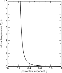
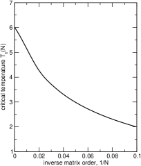
Figure 9: Critical temperatures $T_{c}$ found numerically vs. the power law exponent $\gamma$ (left panel). Right panel represents the dependence of $T_{c}$ on the matrix size $N$ extrapolated to $1/N\rightarrow 0$ for $\gamma=1/4$; behavior for other $\gamma$ is similar; left panel shows $T_{c}$ already extrapolated to $1/N\rightarrow 0$.}

References

- (1) A. Damascelli, Z. Hussain, and Z.X. Shen, Rev. Mod. Phys. 75, 473 (2003).
- (2) G. Blumberg, A. Koitzsch, A. Gozar, B. S. Dennis, C. A. Kendziora, P. Fournier, and R. L. Greene, Phys. Rev. Lett. 88, 107002 (2002); ibid. 90, 149702 (2003).
- (3) S.V. Dordevic and D.N. Basov, cond-mat/0510351 (unpublished) and references therein.
- (4) Y. Onose, Y. Taguchi, K. Ishizaka, and Y. Tokura, Phys. Rev. B 69, 024504 (2004).
- (5) A. J. Millis, A. Zimmers, R. P. S. M. Lobo, N. Bontemps, and C. C. Homes, Phys. Rev. B 72, 224517 (2005).
- (6) D. van der Marel, H. J. A. Molegraaf, J. Zaanen, Z. Nussinov, F. Carbone, A. Damascelli, H. Eisaki, M. Greven, P. H. Kes, M. Li, Nature 425, 271 (2003).
- (7) C. Homes, unpublished
- (8) Z-X Shen, D. Dessau et al, Phys. Rev. Lett. 70, 1533 (1993); H. Ding, Phys. Rev. B54, R9678 (1996).
- (9) H. Matsui, K. Terashima, T. Sato, T. Takahashi, M. Fujita, and K. Yamada, Phys. Rev. Lett. 95, 017003 (2005).
- (10) L. Alff, Y. Krockenberger, B. Welter, M. Schonecke, R. Gross, D. Manske, M. Naito, Nature 422, 698 (2003).
- (11) Y Tokura, H. Takagi, S. Uchida , Nature 337, 345 (1989).
- (12) A. Koitzsch, G. Blumberg, A. Gozar, B. S. Dennis, P. Fournier, and R. L. Greene, Phys. Rev. B67, 184522 (2003).
- (13) A. Zimmers, J. M. Tomczak, R. P. S. M. Lobo, N. Bontemps, C. P. Hill, M. C. Barr, Y. Dagan, R. L. Greene, A. J. Millis and C. C. Homes, Europhys. Lett. 70, 225 (2005).
- (14) P. Coleman and C. Pepin, Acta Physica Polonica B 34, 691 (2003).
- (15) Y. Dagan, M. M. Qazilbash, C. P. Hill, V. N. Kulkarni, and R. L. Greene, Phys. Rev. Lett. 92, 167001 (2004).
- (16) D.J. Scalapino, Phys. Rep. 250, 329 (1995); P. Monthoux and D. Pines, Phys. Rev. B 47, 6069 (1993).
- (17) D. Manske, I. Eremin, and K.H. Bennemann, Phys. Rev. B 62, 13922 (2000).
- (18) A. Abanov, A. V. Chubukov, and J. Schmalian, Adv. Phys. 52, 119 (2003).
- (19) Ar. Abanov, A. V. Chubukov and A. M. Finkel’stein, Europhys. Lett., 54, 488 (1999)
- (20) R.S. Markiewicz, in Intrinsic Multiscale Structure and Dynamics in Complex Electronic Oxides, ed. by A.R. Bishop, et al., World Scientific (2003).
- (21) F. Onufrieva and P. Pfeuty, Phys. Rev. Lett. 92, 247003 (2004).
- (22) B.L. Altshuler, L.B. Ioffe, A.J. Millis, Phys. Rev. B 52, 5563 (1995).
- (23) V. A. Khodel, V. M. Yakovenko, M. V. Zverev, and H. Kang, Phys. Rev. B 69, 144501 (2004).
- (24) K. Yoshimura and D.S. Hirashima, J. Phys. Soc. Jpn. 74, 712 (2005) and references therein.
- (25) P. Krotkov and A.V. Chubukov, Phys. Rev. Lett. 96, 107002 (2006).
- (26) A. Virosztek and J. Ruvalds, Phys. Rev. B 42, 4064 (1990).
- (27) The self-energy at finite temperature has been obtained by O. Tchernyshyov and A.V. Chubukov (unpublished).
- (28) B. L. Altshuler, L. B. Ioffe, and A. J. Millis, singular fermions.
- (29) A.V. Chubukov, C. Pepin, and J. Rech, Phys. Rev. Lett. 92, 147003 (2004).
- (30) R. Hlubina, T. M. Rice, Phys. Rev. B51, 9253 (1995).
- (31) M.R. Norman and A.V. Chubukov, Phys. Rev. B 73, 140501 (R) (2006).
- (32) M. M. Qazilbash, A. Koitzsch, B. S. Dennis, A. Gozar, Hamza Balci, C. A. Kendziora, R. L. Greene, G. Blumberg, cond-mat/0510098, to be published in PRB.
- (33) A symmetric in solution of (33) that would correspond to a wave gap stipulates a different overall sign before the kernel; and an odd-frequency wave solution has lower than the even-frequency one.
- (34) Ar. Abanov, B.L. Altshuler, A.V. Chubukov, and J. Schmalian, (unpublished).
- (35) W. H. Press, B. P. Flannery, S. A. Teukolsky, W. T. Vetterling, Numerical Recipes: The Art of Scientific Computing, New York, 2002.
- (36) Ar. Abanov, A. V. Chubukov, M. Eschrig, M. R. Norman, and J. Schmalian, Phys. Rev. Lett, 89, 177002 (2002).