Chemical etching of a disordered solid: from experiments to field theory.

Abstract

We present a two-dimensional theoretical model for the slow chemical corrosion of a thin film of a disordered solid by suitable etching solutions. This model explain different experimental results showing that the corrosion stops spontaneously in a situation in which the concentration of the etchant is still finite while the corrosion surface develops clear fractal features. We show that these properties are strictly related to the percolation theory, and in particular to its behavior around the critical point. This task is accomplished both by a direct analysis in terms of a self-organized version of the Gradient Percolation model and by field theoretical arguments.

1 Introduction

When an etching solution is put in contact with a disordered etchable solid, it corrodes the “weak” parts of the solid surface while the “hard” parts remain un-corroded. During this process new regions of the solid (both hard and weak) are discovered coming into contact with the etching solution. If the volume of the solution is finite and the etchant is consumed in the chemical reaction, the etching power of the solution diminishes progressively and the corrosion rate slows down. When the solution is too weak to corrode any part of the hardened solid surface, the dynamics spontaneously stops. It is an experimental observation Balazs that the etchant concentration at the arrest time is larger than zero. We show below that its value is strictly related to the percolation threshold of the considered solid lattice. We show also that the final connected solid surface has clear fractal features up to a certain characteristic scale $\sigma$, i.e., the surface thickness. This is precisely the phenomenology that has been recently observed in experiments on pit corrosion of aluminum thin films Balazs . We show that the fractal features and the characteristic scale can be explained by the critical behavior of classical percolation around the percolation threshold Aharony .

2 The model

A simple dynamical model, capturing the above mentioned phenomenology, has been recently proposed and studied model ; GBS .

Figure 1: Sketch of the etching dynamics in a square lattice: the sites $2,3,5$ are etched at the first time-step as their resistances are lower than $p(0)$. At the same time the number of etchant particles in the solution decreases by $3$ units, and a new part of the solid is uncovered.

The model is sketched in Fig. 1, and can be formulated as follows:
(i) The solid is represented by a square lattice of sites with random resistances to corrosion $r_{i}$ uniformly distributed in the interval $[0,1]$. It has a width $L$ and a given fixed depth $Y$. The etching solution has a finite constant volume $V$, and contains an initial number $N_{et}(0)$ of etchant molecules: the initial etchant concentration is therefore $C(0)=N_{et}(0)/V$. Experimentally the “etching power” $p(t)$ of the solution at time $t$ is roughly proportional to the concentration $C(t)$. We assume $p(t)=C(t)$ without loss of generality, and take $p_{c}<p(0)\leq 1$, where $p_{c}$ is the percolation threshold of the lattice.
(ii) At $t=0$ the solution is put in contact with the solid through the bottom boundary $y=0$. At each time-step $t$, the solid sites belonging to the solid-solution interface with $r_{i}<p(t)$ are removed, and a particle of etchant is consumed for each corroded site. Consequently, the concentration of the solution decreases with $t$. Finally, depending on the connectivity criterion chosen for the lattice sites (e.g., first nearest neighbor connectivity for solid sites), $m(t)$ new solid sites, previously in the bulk, come into contact with the solution for the first time. At the next time-step, only these sites can be corroded, as the other surface sites have already resisted to etching and $p(t)$ decreases with $t$. Calling $n(t)$ the number of removed solid sites at time $t$, and $N(t)$ the total number of removed sites up to time $t$, one can write

$$p(t+1)=p(t)-\frac{n(t)}{V}=p(0)-\frac{\sum_{t^{\prime}=0}^{t}n(t)}{V}=p(0)-\frac{N(t)}{V}\,.$$ (1)

Note that, during the process, the solution can surround and detach finite solid islands from the bulk. The global solid surface is then composed by the union of the perimeter of the “infinite” solid, here called corrosion front, and the surfaces of the finite islands. At the end, the corrosion dynamics spontaneously stops at $t_{f}$ such that all the surface sites have resistances $r>p(t_{f})$.

The main features of the model, found through extensive numerical simulations (lattices with up to $2000\times 2000$ solid sites in GBS ), are:
(i) The final value $p_{f}=p(t_{f})$ is slightly smaller than the percolation threshold $p_{c}$. The difference $|p_{f}-p_{c}|\rightarrow 0$ as $(L/V)^{\alpha_{p}}$ (we take $L/V\ll 1$) with $\alpha_{p}\simeq 0.45$, when the limits $L,V\rightarrow+\infty$ are taken in the appropriate way GBS . All this can be explained through percolation theory which, in fact, implies that for $p(t)\leq p_{c}$ the probability to have a connected path of solid sites all with $r>p(t)$ (and then stopping corrosion) is equal to one in the infinite volume limit.

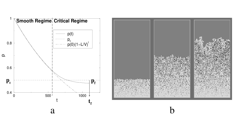
Figure 2: a- Time decay of $p(t)$ (continuous line), compared to the analytical approximation $p(t)=p_{0}\exp(-tL/V)$ in the smooth regime (dashed line) GBS in a triangular lattice. There is good agreement for $p(t)>p_{c}$. b- Three snapshots of the corroded solid (dark gray) by the solution (clear) at three different time-steps: initial, intermediate and final. Black regions represent detached islands. The final corrosion front shows fractality up to a scale given by its thickness.

(ii) The corrosion dynamics can be divided (see Fig. 2-a) into two regimes: a smooth regime when $p(t)>p_{c}$, and a critical regime when $p(t)\simeq p_{c}$. The duration of the former is measured approximately by $t_{c}$, defined by $p(t_{c})=p_{c}$; $t_{c}$ is found to scale with the ratio $L/V$ in the following way $t_{c}\sim V/L$. The duration of the latter, $(t_{f}-t_{c})$, scales as $(V/L)^{\alpha_{t_{f}}}$ with $\alpha_{t_{f}}\simeq 0.55$ (with a further linear dependence on $\log\,L$ of the scaling coefficient due to the extremal nature of $t_{f}$ frac ).
(iii) The surface of the solid in contact with the solution displays a peculiar roughening dynamics (see Fig. 2-b). In the first smooth regime, the corrosion has a clear mean direction given by the initial condition, and the corrosion front becomes progressively rougher and rougher, while finite detached islands are quite small. In the second critical regime, spatial correlations increase on the corrosion front and the dynamics generates a locally isotropic fractal geometry, while the detached islands are larger.

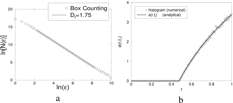
Figure 3: a-Box counting measure of the fractal dimension of the corrosion front for length smaller than $\sigma$. b-Final normalized histogram of the global solid surface: simulations results (empty points) are compared with the analytical evaluation (continuous line).

(iv) The final corrosion front is fractal with a fractal dimension $D_{f}=1.753\pm 0.05$ (see Fig. 3-a) up to a characteristic scale $\sigma$ which is the final thickness of the front. On larger scales the corrosion front looks like a one-dimensional line. Also $\sigma$ scales with $L/V$ as follows: $\sigma\sim(L/V)^{-\alpha_{\sigma}}$ with $\alpha_{\sigma}\simeq 0.57\simeq 1/D_{f}$. All these properties are well explained in the framework of percolation theory as a self-organized version of the Gradient Percolation model GP ; GBS .
(v) Another important experimental observation captured by this simple model is the progressive hardening of the solid surface, due to the corrosion only of freshly discovered weak sites which, in turn, deplete the etchant concentration in time permitting future corrosion of only weaker sites. This hardening effect is described quantitatively by the behavior of the normalized resistance histogram $\phi(r,t)$ of the global surface sites giving the density of such sites with resistance $r$. Obviously, $\phi(r,0)=1$ with $r\in[0,1]$, while $\phi(r,t_{f})$ is given in Fig. 3-b. As one can see, the final global surface is much more resistant to corrosion than the initial one. The time evolution and the final shape of $\phi(r,t)$ have been successfully obtained theoretically in GBS .

3 Field theory approach and dynamical percolation

In order to describe this model in the critical regime, it is possible to develop a phenomenological field theory approach “à la Landau” (see Munoz ) consisting in writing down the functional Langevin equation of the process around criticality directly from the analysis of the symmetries of the system. To this aim let us consider the following three different local densities or coarse-grained fields:
(i) $s({\bf x},t)$ describing the local density in the point ${\bf x}$ at time $t$ of material susceptible to be etched at any time after $t$ (i.e., in the discrete model presented above, bulk solid sites and “fresh” solid surface sites freshly arrived to the solid-liquid interface).
(ii) $q({\bf x},t)$ is the local density of passivated and inert material (i.e., surface solid sites having already resisted an etching trial and then immune or not-susceptible to be corroded at any future time-step).
(iii) $c({\bf x},t)$ is the local density of corroded sites replaced by solution sites.

The mean field equations (rate equations) describing the evolution of the averaged mean values of these magnitudes are to the leading order in the fields Munoz :

$$\dot{s}(t) = -\alpha c(t)s(t)$$

$$\dot{q}(t) = \alpha(1-p(t))c(t)s(t)$$

$$\dot{c}(t) = \alpha p(t)c(t)s(t)$$ (2)

where $p(t)$ is the probability to etch an active site at time $t$, and $\alpha$ is a positive constant that we fix equal to one without loss of generality. The interpretation of the first equation is: in order for the density of susceptible sites to change (decrease) in a region, it is necessary to have locally both a non-vanishing density of etchant and raw solid material susceptible to be etched. This restricts the dynamics to active regions (i.e., part of the solution-solid interface) in which non-vanishing local densities of $s$ and of $c$ coexist. The second and the third relations in Eq. 2 say that an active site becomes either a $c$-site, with probability $p(t)$, or alternatively, after healing, a $q$-site with complementary probability $1-p(t)$. Note that, as $\dot{s}~{}+~{}\dot{c}~{}+~{}\dot{q}~{}=~{}0$, the total number of sites is conserved during the dynamics. We have written so far mean field equations in which spatial dependence and fluctuations are not taken under consideration. To this aim, it is convenient to introduce the activity field $\rho({\bf x},t)\equiv c({\bf x},t)s({\bf x},t)$. From Eq. 2 it follows immediately that

$$\dot{\rho}(t)=-c(t)\rho(t)+p(t)s(t)\rho(t)\,.$$ (3)

We now use for $p(t)$ Eq. 1, noting that in terms of the coarse grained fields we have $N(t)=\int d{\bf x}[c({\bf x},t)-c({\bf x},0)]$. Using this observation, it is simple to derive the expression of $p(t)$ as a function of the activity field $\rho({\bf x},t)$:

$$p(t)=p(0)\exp\left[-{1\over V}\int_{0}^{t}dt^{\prime}\int_{V}d{\bf x}\rho({\bf x},t^{\prime})\right]=p(0)\exp\left[-\int_{0}^{t}dt^{\prime}\overline{\rho}(t^{\prime})\right]\,,$$ (4)

where $\overline{\rho}(t)={1\over V}\int d{\bf x}\rho({\bf x},t)$ is the average activity at time $t$. Since $p(t)$ is a function only of the average activity, it can be considered as a deterministic, smooth, positive and decreasing term in the final Langevin equation, even though $\rho({\bf x},t)$ is a stochastic field. Using Eqs. 2, 3 and 4 it is possible to write the mean field equation for the activity field:

$$\partial_{t}\rho({\bf x},t)=m(t)\rho({\bf x},t)-\rho({\bf x},t)\int_{0}^{t}dt^{\prime}(p(t)+p(t^{\prime}))\rho({\bf x},t^{\prime})\,,$$ (5)

where $m(t)=p(t)s({\bf x},0)-c({\bf x},0)$. In order to obtain the complete functional Langevin equation (i.e., the field theory) for the process in the neighborhood of the critical point (i.e., $p(t)\simeq p_{c}$), we have to add to Eq. 5 the noise term and the spatial coupling terms. The former is found simply by observing that, if in a local region there are $k$ etchable sites in contact with the solution at time $t$, an average number $p(t)k$ of them will be etched with a typical Poissonian fluctuation of the order of $\sqrt{p(t)M}$. This shows that the noise term is $\sim\sqrt{\rho({\bf x},t)}\eta({\bf x},t)$ (multiplicative noise), where $\eta({\bf x},t)$ is the typical white uncorrelated noise with zero mean and $\left<\eta({\bf x},t)\eta({\bf x^{\prime}},t^{\prime})\right>=A\delta({\bf x}-{\bf x^{\prime}})\delta(t-t^{\prime})$. As a consequence of Eq. 5 and of the form of the noise term, it is possible to show that the only relevant term of spatial coupling in the neighborhood of the critical point is the diffusion term $\nabla^{2}\rho({\bf x},t)$. Since $p(t)$ is smooth, positive and, in the neighborhood of the critical point, $p(t)\simeq p_{c}>0$, at the end we obtain a field theory that belongs to the universality class of dynamical percolation (i.e., of a dynamical version of the classical percolation) dyn-perc :

$$\partial_{t}\rho({\bf x},t)\!=\!m\rho({\bf x},t)\!-\!\gamma\rho({\bf x},t)\!\int_{0}^{t}dt^{\prime}\rho({\bf x},t^{\prime})\!+\!\nabla^{2}\rho({\bf x},t)\!+\!\sqrt{\rho({\bf x},t)}\eta({\bf x},t)\,,$$ (6)

where $\gamma>0$, and $m$ measures, in the dynamical percolation ,the distance $p-p_{c}$ between the chosen constant occupation probability $p$ and its critical value $p_{c}$. If $m>0$ —active phase— the process generate an infinite cluster of occupied sites, and if $m<0$ —absorbing state absorbing — the occupation process arrests exponentially fast (i.e., $\rho({\bf x},t)$ decreases rapidly to zero) leaving only a finite cluster of occupied sites. Since $\rho({\bf x},t)\equiv 0$ is a solution of Eq. 6, once this state is reached the occupation dynamics (i.e., in our model the corrosion) stops spontaneously: $\rho({\bf x},t)=0$ is a so-called an absorbing state, and at $m=0$ we have an “absorbing state phase transition”. However, in our case (Eq. 5) $m$ depend on time, and starting with a positive value, as $p(t)$ decreases in time, it passes spontaneously from the active phase ($m>0$) to the absorbing phase ($m<0$) arresting rapidly after this crossover. The velocity of this crossover, that is, the duration of the critical regime, depends on the finite size of the system which in this way determine both the effective spatial gradient of $p$ and the typical scale of fractality of the system, while the critical exponents are those of percolation theory Munoz . This shows, finally, that our model is a self-organized version of Gradient Percolation in any dimension.

References

- (1) L. Balázs, Phys. Rev. E 54, 1183 (1996).
- (2) D. Stauffer and A. Aharony, Introduction to Percolation Theory, 2 ed., Taylor & Francis Ltd., London (1991).
- (3) B. Sapoval, S. B. Santra and P. Barboux, Europhys. Lett., 41, 297, (1998).
- (4) A. Gabrielli, A. Baldassarri, and B. Sapoval, Phys. Rev. E. 62, 3103 (2000).
- (5) A. Baldassarri, A. Gabrielli, and B. Sapoval, Europhys. Lett. 59, 232 (2002).
- (6) B. Sapoval, M. Rosso, and J. F. Gouyet, J. Phys. Lett. (Paris), 46, L149 (1985).
- (7) A. Gabrielli, M. A. Muñoz, and B. Sapoval, Phys. Rev. E 64, 016108 (2001).
- (8) H. Saleur, and B. Duplantier, Phys. Rev. Lett., 58, 2325 (1986).
- (9) H. K. Janssen, Z. Phys. B 58, 311 (1985).
- (10) H. Hinrichsen, Adv. Phys. 49, 815 (2000).