Hopping conductivity of a suspension of nanowires in an insulator

Abstract

We study the hopping conduction in a composite made of straight metallic nanowires randomly and isotropically suspended in an insulator. Uncontrolled donors and acceptors in the insulator lead to random charging of wires and, hence, to a finite bare density of states at the Fermi level. Then the Coulomb interactions between electrons of distant wires result in the soft Coulomb gap. At low temperatures the conductivity is due to variable range hopping of electrons between wires and obeys the Efros-Shklovskii (ES) law $\ln\sigma\propto-(T_{ES}/T)^{1/2}$. We show that $T_{ES}\propto 1/(nL^{3})^{2}$, where $n$ is the concentration of wires and $L$ is the wire length. Due to enhanced screening of Coulomb potentials, at large enough $nL^{3}$ the ES law is replaced by the Mott law.

In recent years, electron transport in composites made of metallic granules surrounded by some kind of insulator generated a lot of interest in both fundamental and applied research. Conductivities of the composites with spherical or generally speaking single scale granules are well studied (see review Vinokur and references therein). If the number of granules $n$ per unit volume is large, granules touch each other and the conductivity is metallic. When $n$ is smaller than the percolation threshold $n_{c}$, granules are isolated from each other, the composite is on the insulating side of metal-insulator transition and the conductivity is due to hopping. It was observed that in this case, the temperature dependence of the conductivity $\sigma$ obeys

$$\sigma=\sigma_{0}\exp[-(T_{0}/T)^{\alpha}],$$ (1)

where $T_{0}$ is a characteristic temperature and $\alpha=1/2$. This behavior of conductivity $\sigma$ was interpreted as the Efros-Shklovskii (ES) variable range hopping (VRH) between granules Zhang ; Vinokur . The finite bare density of states at the Fermi level was attributed to the charged impurities in the insulator playing the role of randomly biased gates. Then the interaction of electrons residing on different dots creates the Coulomb gap, which leads to ES variable range hopping.

For needle-like granules such as metallic whiskers or metallic nanotubes, the experimental situation is more complicated than for single scale ones. Recently ES temperature dependence of the conductivity was reported Benoit for composites made of bundles of single-wall carbon nanotubes (SWNT) suspended in insulating polymers. On the other hand, the Mott law with $\alpha=1/4$ was also observed in many nanotube based materials Benoit ; Gaal ; Fuhrer ; Yosida . In order to understand the puzzling crossover between ES and Mott hopping, in this paper, we study the low temperature ohmic dc transport in an isotropic suspension of elongated metallic granules in an insulating medium (see Fig. 1). Below we call such a granule a wire for brevity.

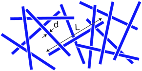
Figure 1: A suspension of neutral metallic wires in an insulator with concentration $1/L^{3}\ll n\ll 1/L^{2}d$.

In this paper we restrict ourselves to scaling approximation for the conductivity and to delineating the corresponding scaling regimes. In our scaling theory, we drop away both all numerical factors and, moreover, also all the logarithmic factors, which do exist in this problem, because it deals with strongly elongated cylinders. In this context, we will use symbol “$=$” to mean “equal up to a numerical coefficient or a logarithmic factor”.

We assume each wire is a cylinder with the length $L$ and the diameter $d\ll L$. When the concentration of wires $n$ is very small, the distance between them is much larger than $L$, we can easily apply the results obtained in the Ref. Zhang . Here we consider a range of concentrations $1/L^{3}\ll n\ll 1/L^{2}d$, where $n$ is so large that spheres built on each wire as the diameter strongly overlap, but the system is still far below the percolation threshold $n_{c}=1/L^{2}d$. Percolation threshold at very small concentration $n_{c}=1/L^{2}d$ is the result of large excluding volume $L^{2}d$ which one wire creates for centers of others. (At concentrations above $1/L^{2}d$ it also becomes impossible to place wires randomly and isotropically because of nematic ordering Onsager , but there is no such problem at $n\ll n_{c}$). Our results are summarized in Fig. 2 in the plane of parameters $T$ and $nL^{3}$. The main result is that at low temperatures, we arrive at ES law

$$\sigma=\sigma_{0}\exp[-(T_{ES}/T)^{1/2}]$$ (2)

with

$$T_{ES}=\frac{e^{2}}{\kappa a(nL^{3})^{2}},$$ (3)

where $\kappa$ is the dielectric constant and $a$ is the tunneling decay length in the insulator. The large factor $(nL^{3})^{2}$ in Eq. (3) is a result of the enhancement of both the effective dielectric constant and the localization length in the composite. At large enough $nL^{3}$ and higher temperatures, ES law is replaced by the Mott law. And when the temperatures are sufficiently high, both VRH regimes are replaced by the activated nearest neighboring hopping (NNH) regimes.

Let us start from the dielectric constant of the composite. In the range of concentrations $1/L^{3}\ll n\ll 1/L^{2}d$, its macroscopic dielectric constant $\kappa_{\rm eff}$ is greatly enhanced due to polarization of long metallic wires. It was shown in the Ref Sarychev ; conductivity , that

$$\kappa_{\rm eff}=(nL^{3})\kappa.$$ (4)

Such result can be understood in the following way. If the wave vector $q$ is larger than $1/L$, the static dielectric function for the wire suspension has the metal-like form

$$\epsilon(q)=\kappa\left(1+\frac{1}{q^{2}r_{s}^{2}}\right),$$ (5)

where $r_{s}=(nL)^{-1/2}$ is the typical separation of the wire from other wires. It plays the role of screening radius for the wire charge. The function $\epsilon(q)$ grows with decreasing $q$ until $q=1/L$ where the composite loses its metallic response and $\epsilon(q)$ saturates. As a result, the macroscopic effective dielectric constant is given by $\kappa_{\rm eff}=\epsilon(q=1/L)=nL^{3}\kappa$. Within our scaling approximation, one can also derive Eq. (4) starting from the facts that each isolated wire has polarizability equal to $L^{3}$ and due to random positions of wires the acting electric field does not differ from the average one.

The spacing between charging energy levels of such wire is the order of $E_{c}=e^{2}/\kappa_{\rm eff}L=e^{2}/\kappa nL^{4}$. If the wire is thick enough, it can be treated as a three dimensional object and the mean quantum level spacing $\delta$ in the wire is the order of $\lambda_{F}\hbar^{2}/mLd^{2}$, where $\lambda_{F}$ is the Fermi wavelength and $m$ is the effective electron mass. Narrow wires such as SWNT with single conducting channel will be discussed later. Using the tunneling decay length $a$ in the insulator, we can rewrite $\delta$ in the form $\delta=\beta e^{2}a^{2}/\kappa d^{2}L$ where $\beta=\lambda_{F}/a$. The ratio $E_{c}/\delta$ decreases proportional to $1/nL^{3}$ because of enhanced screening of Coulomb interaction in the denser system of longer wires.

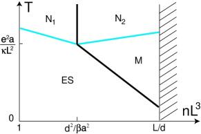
Figure 2: (Color online) The summary of the transport regimes for relatively clean wires schematically plotted in the plane of $nL^{3}$ and temperature $T$. The dark line separates regimes where Coulomb interaction is important ($\rm N_{1}$ [Eq. (7)] and ES law [Eq. (2)]) from regimes where it plays a minor role ($\rm N_{2}$ [(10)] and Mott (M) law [Eq. 8]). The grey (blue) line separates activated the nearest neighbor hopping (NNH) regimes from the VRH regimes. Shaded domain represents the metallic side of the insulator-metal transition. Instead of smooth crossovers at dark and grey lines, in the vicinity of this transition, the conductivity has a critical behavior.

We start our discussion with relatively small $nL^{3}$ such that $nL^{3}<d^{2}/\beta a^{2}$ and $E_{c}\gg\delta$. The density of states and localization length are all the information we need to calculate the VRH conductivity. In contrary to a doped semiconductor, in a suspension of neutral wires, the bare density of states at the Fermi level $g_{0}=0$. Charging energy levels of the suspended wires are shown in Fig. 3(a), they are equally spaced by $E_{c}$. The Fermi level is at zero energy between empty and filled levels.

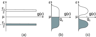
Figure 3: The density of ground states at $E_{c}\gg\delta$. (a) BDOGS in neutral wires, (b) BDOGS for charged wires with large enough concentration of donors in the insulator in the absence of the long range Coulomb interaction; (c) The density of ground states of charged wires with the Coulomb gap in the vicinity of the Fermi level $\mu$. Occupied states are shaded.

Since the ground states of wires determine the low temperature hopping transport, we consider only the ground state in each wire at a given number of electrons and exclude excited states Zhang . Thus, the density of states we need can be called bare density of ground states (BDOGS). According to Ref. Zhang , the finite BDOGS near the Fermi level originates from uncontrollable donors (or acceptors) in the insulating host. Donors have the electron energy above the Fermi energy of wires. Therefore, they donate electrons to wires. A positively charged ionized donor can attract and effectively bind fractional negative charges on all neighboring wires, leaving the rest of each wire fractionally charged. At a large enough average number ($\gg 1$) of donors per wire, effective fractional charges on different wires are uniformly distributed from $-e/2$ to $e/2$. In such a way the Coulomb blockade in a single wire is lifted and the discrete BDOGS get smeared (see Fig. 3(b)). The BDOGS $g_{0}$ becomes $1/E_{c}L^{3}$. In the very vicinity of the Fermi energy, the long range Coulomb interaction creates the parabolic Coulomb gap $\Delta$ (see Fig. 3(c)). The Coulomb gap affects energy interval $|\epsilon|\lesssim\Delta$. At low enough $T$, when the range of energy levels around the Fermi level responsible for hopping $(T_{ES}T)^{1/2}$ is much smaller than $\Delta$, the conductivity obeys the ES law (see Eq. (2)) and does not depend on $g_{0}$ ES . The parameter $T_{ES}=e^{2}/\kappa_{\rm eff}\xi$, where $\xi$ is the localization length for tunneling to distances much larger than $L$. Let us concentrate now on the nontrivial value of the localization length $\xi$.

It was suggested Boris that such long range hopping process can be realized by tunneling through a sequence of wires (see Fig. 4). The states of the intermediate wires participate in the tunneling process as virtual states. Nowadays the virtual electron tunneling through a single granule is called co-tunneling Nazarov ; Ioselevich ; Beloborodov ; Vinokur ; Fogler1 and regarded as a key mechanism of low temperature charge transport via quantum dots. One should distinguish the two co-tunneling mechanisms, elastic and inelastic. During the process of elastic co-tunneling, the electron tunneling through an intermediate virtual state in the granule leaves the granule with the same energy as its initial state. On the contrary, the tunneling electron in the inelastic co-tunneling mechanism leaves the granule with an excited electron-hole pair behind it. Which mechanism dominates the transport depends on the temperature. Inelastic co-tunneling dominates at $T>\sqrt{E_{c}\delta}$, while below this temperature, elastic co-tunneling wins. In discussions below, we consider sufficiently low temperatures such that only elastic co-tunneling is involved.

First we remind the idea of calculation of the localization length $\xi$ used in Ref. Boris . (Such approach was also applied in the papers Zhang ; Fogler ). When an electron tunnels through the insulator between wires at the nearest neighboring hopping (NNH) distance $r$, it accumulates dimensionless action $r/a$, where $a$ is the tunneling decay length in the insulator. We want to emphasize that the NNH distance $r$ is realized only in one point of the wire and, therefore, is much shorter than the typical separation along the wire from other wires $r_{s}$. NNH distance $r$ can be calculated using the percolation method ES . If one builds around each wire a cylinder with length $L$ and radius $r$, percolation through these cylinders appears, when $nL^{2}r=1$. This happens because excluded volume created by one cylinder is not $r^{2}L$, but $L^{2}r$. As a result, we obtain $r=1/nL^{2}$. We assume the metallic wire is only weakly disordered and hence we neglect the decay of electron wave function in the wire. (This assumption will be relaxed later.) Over distance $x$, electron accumulates $x/L$ additive actions of the order of $r/a$. Thus, its wave function decays as $\exp(-xr/La)=\exp(-x/\xi)$, where the localization length $\xi=aL/r=a(nL^{3})$. This contributes another factor $nL^{3}$ to Eq. (3). Eq. (2) with $T_{ES}$ given by Eq. (3) is valid in the left lower corner of Fig. 2 labeled as ES. More rigorous calculation Beloborodov of the localization length $\xi$ gives $\xi=L/[\ln(E_{c}\pi/\delta)+1/nL^{2}a]$. Our simple derivation of $\xi$ along the line of Ref. Boris has lost the first term in the denominator. We argue that in our case $1/nL^{2}a\gg d/a$, and $d/a$ can be quite large. As a result, within a large range of the ratio $E_{c}/\delta$, the term $\ln(E_{c}\pi\delta)$ is only a small correction to the leading term $1/nL^{2}a$.

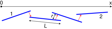
Figure 4: (Color online) An illustration of a long range ($\gg L$) hop from the wire 1 to the wire 2 via a sequence of wires.

At high temperatures, the conductivity is dominated by the nearest neighbor hopping. Using the NNH distance $r$, we obtain the conductivity with activated $T$-dependence,

$$\sigma\propto{\rm e}^{-1/nL^{2}a}{\rm e}^{-E_{A}/T},$$ (6)

where the activation energy $E_{A}$ is determined by the charging energy

$$E_{A}=\frac{e^{2}}{\kappa_{\rm eff}L}=\frac{e^{2}}{\kappa nL^{4}}\ \ \ {\rm if}\ \ \ \delta\ll E_{c}.$$ (7)

The range of validity of Eqs. (6) and (7) is shown in the upper left corner of Fig. 2 and labeled as $\rm N_{1}$.

When $L$ becomes so large that $\delta>E_{c}$, the BDOGS $g_{0}$ evolves from $(E_{c}L^{3})^{-1}$ to $g_{0}=(\delta L^{3})^{-1}=\kappa d^{2}/e^{2}\beta L^{2}a^{2}$. Since $g_{0}$ decreases and $\kappa_{\rm eff}$ grows with $L$, the width of the Coulomb gap $\Delta$, which can be estimated as $=\sqrt{g_{0}e^{6}/\kappa_{\rm eff}^{3}}$ decreases with $L$. Eventually, the Coulomb gap becomes narrower than the width of Mott’s optimal band $\epsilon_{M}=T^{3/4}/(g_{0}\xi^{3})^{1/4}$ at given $T$. At this point, the ES law is replaced by the conventional Mott’s law,

$$\sigma=\sigma_{0}\exp[-(T_{M}/T)^{1/4}],$$ (8)

where

$$T_{M}=\frac{1}{g_{0}\xi^{3}}=\frac{\beta e^{2}}{\kappa an^{3}L^{7}d^{2}}.$$ (9)

This regime is labeled as M in Fig. 2. It crossover to the ES regime at $T=e^{2}d^{2}/\kappa a\beta nL^{5}$, which can be obtained by equating $\Delta$ and $\epsilon_{M}$. This change of the temperature dependence of the conductivity from $1/2$ ES law to $1/4$ Mott law was observed at relatively high temperatures and large concentrations in the experiment Benoit .

At high temperatures, the Mott’s law is replaced by the NNH conductivity with activation energy equal to the spacing of quantum levels $\delta$. The $T$-dependence of the conductivity is,

$$\sigma\propto\exp\left(-\frac{1}{nL^{2}a}\right)\exp\left(-\frac{e^{2}\beta a^{2}}{\kappa d^{2}LT}\right),\ \ \ {\rm if}\ \ \ \delta\gg E_{c}.$$ (10)

We call this regime $\rm N_{2}$ and show it in the right upper corner of Fig. 2. It is easy to check that ES and Mott VRH transport regimes match corresponding NNH regimes $\rm N_{1}$ and $\rm N_{2}$ smoothly, when VRH distance is of the order of the wire length $L$. This happens at the gray line of Fig. 2. The Coulomb regimes ES and $\rm N_{1}$ smoothly crossover to the regimes M and $\rm N_{2}$ of noninteracting electrons at the dark line of Fig. 2. We stop at $nL^{3}=L/d$, where percolation leads to the insulator-metal transition. Our scaling approach is not designed to study the critical behavior of the conductivity in the vicinity of the transition.

Now we switch to the case of metallic wires with a strong internal disorder, where the electron wave function decay length $\lambda$ is much smaller than the wire length $L$. The summary of transport regimes for this case is presented in Fig. 5. In order to show all the possible regimes, we assume that $\lambda$ is small enough for the order of labels on the $nL^{3}$ axis shown in Fig. 5. (At a larger $\lambda$ only some of the shown regimes may exist.) We also plotted regimes labeled as ES and $\rm N_{1}$ on the left of the border line $nL^{3}=n\lambda^{3}$. The characteristic energies of electron transport in these regimes are given by Eqs. (3) and (7) respectively.

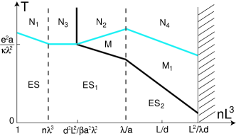
Figure 5: (Color online) Transport regimes for wires, where electrons are localized at length $\lambda<L$. Dark line separates regimes where Coulomb interaction is important ($\rm N_{1,3}$ and ES laws) from regimes where it plays minor role ($\rm N_{2,4}$ and Mott laws). The grey (blue) line separates activated NNH regimes from VRH regimes. The left dashed line marks the border where dielectric constant $\kappa_{\rm eff}$ starts growing with $nL^{3}$, while the right dashed line serves as the border where localization length $\xi$ stops growing and becomes $\lambda$. The shaded domain represents the metallic side of the insulator-metal transition. Instead of smooth crossover, in the vicinity of the transition, the conductivity has a critical behavior.

When $L\gg\lambda$, the wires can be treated as a larger number of clean metallic wires with length of the order $\lambda$ and the concentration $nL/\lambda$. Following the logic of Ref. Sarychev and our derivation of $\kappa_{\rm eff}$ (Eq. (4)) one can show that the effective macroscopic dielectric constant is given by

$$\kappa_{\rm eff1}=\kappa nL\lambda^{2}.$$ (11)

Comparing to (Eq. (4)) we see that the dielectric constant $\kappa_{\rm eff1}$ is strongly reduced by the internal disorder of wires. This happens because the disorder effectively ”cuts” the wire into short pieces albeit increases the concentration of the short wires.

The internal disorder also changes the localization length for the long distance ($\gg L$) tunneling. Using the argument we made above, we obtain

$$\frac{1}{\xi}=\frac{1}{\lambda}+\frac{1}{nL^{3}a},$$ (12)

where the first term on the right hand side accounts for the decay of the wave function in the wire, while the second term represents the decay in the insulating medium between the wires. When $nL^{3}<\lambda/a$, the second term dominates, $\xi=nL^{3}a$, which is the same as what we got for the case of clean wire. However, because of new dielectric constant $\kappa_{\rm eff1}$ (Eq. 11), we obtain new regime labeled $\rm ES_{1}$ in the Fig. 5. Here the conductivity obeys ES law with the characteristic temperature

$$T_{ES_{1}}=\frac{e^{2}}{\kappa an^{2}L^{4}\lambda^{2}}.$$ (13)

The charging energy $E_{c}$ also changes to $e^{2}/\kappa_{\rm eff1}L=e^{2}/\kappa nL^{2}\lambda^{2}$. It decreases with growing $nL^{3}$ and reaches the mean quantum level spacing $\delta$ of the wire at $nL^{3}=d^{2}L^{2}/\beta a^{2}\lambda^{2}$. With relatively high temperature and small $nL^{3}<d^{2}L^{2}/\beta a^{2}\lambda^{2}$, the regime $\rm ES_{1}$ crossover to the regime $\rm N_{3}$, where the conductivity can be represented by the same equation (6) but with a different activation energy $E_{A}=e^{2}/\kappa nL^{2}\lambda^{2}$. When $nL^{3}>d^{2}L^{2}/\beta a^{2}\lambda^{2}$, the Coulomb interaction plays a minor role. Hopping conductivities in regimes $\rm M$ and $\rm N_{2}$ are not affected by the change of the dielectric constant and are given by the same Eqs. (8), (9) and (6), (10) respectively.

At even larger $nL^{3}>\lambda/a$, the decay of electron wave functions in the wire dominates, thus $\xi=\lambda$. As a result, we have another ES regime, $\rm ES_{2}$, with

$$T_{ES_{2}}=\frac{e^{2}}{\kappa nL\lambda^{3}},$$ (14)

the Mott regime $\rm M_{1}$ with

$$T_{M_{1}}=\frac{e^{2}}{\kappa an^{2}L^{4}\lambda^{2}}.$$ (15)

and the activated nearest neighboring hopping regime $\rm N_{4}$, with the activation energy $\delta$ and

$$\sigma\propto\exp\left(-\frac{L}{\lambda}\right)\exp\left(-\frac{e^{2}\beta a^{2}}{\kappa d^{2}LT}\right).$$ (16)

Thus, we have completed our consideration of the phase diagram up to $nL^{3}=L/d$, at which wires begin to percolate. What happens to the conductivity if one manages to create an isotropic suspension with $nL^{3}>L/d$? In contrary to relatively clean wires, there is no insulator-metal transition around $nL^{3}=L/d$, where wires start to touch each other. Indeed such transition happens when the typical branch of the percolating network is metallic, which means the typical distance between two nearest neighboring contacts along the same wire can not be $L$, but should be smaller than $\lambda$. We can now think about percolation over pieces of wires with the length $\lambda$ and the effective concentration $nL/\lambda$. Such percolation appears at $(nL/\lambda)(\lambda^{2}d)=1$ or $nL^{3}=L^{2}/\lambda d$. This is the threshold of insulator-metal transition. As a result our phase diagram of hopping regimes is extended as far as $nL^{3}=L^{2}/\lambda d$.

In this paper we concentrated on relatively thick wires with the three dimensional density of states. Narrow wires with as few as one conducting channel should be treated as one dimensional objects. In such case the level spacing is given by $\delta=\hbar^{2}/m\lambda_{F}L$ and thus $E_{c}/\delta=(1/nL^{3})(\lambda_{F}/a)=\beta/nL^{3}$. Since most probably $\beta$ is the order of $1$, while $nL^{3}\gg 1$, the charging energy $E_{c}$ is always smaller than level spacing $\delta$. Coulomb interaction plays minor role in such system. Therefore the left part of our phase diagram Fig. 2 including ES regime vanishes.

It is tempting to apply this theory to carbon nanotubes. Metallic SWNT has only one conducting channel. Therefore for them, the domain of ES hoping most likely vanishes. Bundles of SWNT, studied in Ref. Benoit definitely have many channels and our theory should work for them providing the geometry of bundles may be approximated by a set of randomly oriented rigid rods of a given characteristic length $L$. In this case, the range of ES conductivity should exist. ES range may also exist for multi-wall nanotubes, where one can expect many parallel metallic channels.

In this paper, we considered only straight wires. One can generalize this theory to random system of flexible wires formed by interpenetrating Gaussian coils (for example conducting polymers suspended in insulating medium). This theory will be published elsewhere.

We are grateful to M. Fogler, M. Foygel, Y.M. Galperin and A.V. Lopatin for useful discussions.

References

- (1) I.S. Beloborodov, A.V. Loptain, V.M. Vinokur and K.B. Efetov, cond-mat/0603522.
- (2) J. Zhang and B.I. Shklovskii, Phys. Rev. B 70, 115317 (2004).
- (3) J.M. Benoit, B. Corraze and O. Chauvet, Phys. Rev. B 65, R241405 (2002).
- (4) R. Gal, J.P. Salvetat and L. Forr, Phys. Rev. B 61, 7320 (2000).
- (5) M.S. Fuhrer, W. Holmes, P. Delaney, P.L. Richards, S.G. Louie and A. Zettl, Synth. Met. 103, 2529 (1999).
- (6) Y. Yosida and I. Oguro, J. Appl. Phys. 86, 999 (1999).
- (7) L. Onsager, Ann. N.Y. Acad. Sci. 51, 627 (1949).
- (8) A.N. Lagarkov and A.K. Sarychev, Phys. Rev. B 53, 6318 (1996).
- (9) Tao Hu, A.Yu. Grosberg, B.I. Shklovskii, Phys. Rev. B 73, 155434 (2006).
- (10) B.I. Shklovskii and A.L. Efros, Electronic Properties of Doped Semiconductors (Springer-Verlag, Berlin, 1984).
- (11) B.I. Shklovskii, Sov. Phys. Solid State 26, 353 (1984).
- (12) D.V. Averin and Yu.V. Nazarov, Phys. Rev. Lett. 65, 2446 (1990).
- (13) M.V. Feigel’man and A.S. Ioselevich, JETP Lett. 81, 277 (2005).
- (14) M.M. Fogler, S.V. Malinin, and T. Nattermann, cond-mat/0602008.
- (15) I.S. Beloborodov, A.V. Lopatin and V.M. Vinokur, Phys. Rev. B 72, 125121 (2005).
- (16) M.M. Fogler, S. Teber, B.I. Shklovskii, Phys. Rev. B 69, 035413 (2004)