Scrambling of Hartree–Fock Levels as a universal Brownian–Motion Process

Abstract

We study scrambling of the Hartree–Fock single–particle levels and wave functions as electrons are added to an almost isolated diffusive or chaotic quantum dot with electron–electron interactions. We use the generic framework of the induced two–body ensembles where the randomness of the two–body interaction matrix elements is induced by the randomness of the eigenfunctions of the chaotic or diffusive single–particle Hamiltonian. After an appropriate scaling of the number of added electrons, the scrambling of both the HF levels and wave functions is described by a universal function each. These functions can be derived from a parametric random matrix process of the Brownian–motion type. An exception to this universality occurs when an empty level just gets filled, in which case scrambling is delayed by one electron. An explanation of these results is given in terms of a generalized Koopmans’ approach.

Introduction. The single–particle levels and eigenfunctions of a chaotic or diffusive quantum dot without electron–electron interactions follow the predictions of canonical random–matrix theory (RMT) within a band of $\sim g$ levels around the Fermi energy, where $g$ is the dimensionless Thouless conductance rmt98 ; rmp00 . In an almost isolated dot, the screened Coulomb interaction $V$ between electrons must be taken into account. In the constant–interaction (CI) model, $V$ is approximated by the charging energy (a constant for a fixed number of electrons), and a single–particle picture and RMT can again be used. In this paper, we go beyond the CI model and use the Hartree–Fock (HF) approximation. This approximation uses a single–particle picture and yet takes into account both chaotic or diffusive motion and interaction effects beyond the CI model. The HF equations depend on the one–body density and must be solved self–consistently. The resulting HF single–particle levels and eigenfunctions depend on the number of electrons on the dot and, therefore, change (are “scrambled”) as electrons are added to the dot Patel98b ; ag . An experimental signature of scrambling is the saturation of the number of correlated Coulomb–blockade conductance peaks as temperature $T$ increases (without scrambling, that number should rise linearly with $T$) Patel98b .

Chaotic or diffusive motion of the electrons induces randomness in the two–body matrix elements of $V$. For spinless electrons, scrambling is due to the fluctuating part of these matrix elements (the average yields the CI model). The fluctuations depend on $g$ and on the geometry of the dot and are, therefore, non–universal blanter97 . Here we evaluate two statistical measures of scrambling and find them to be also non–universal. This is in accord with expectations based on Koopmans’ limit koopmans34 , where the HF wave functions are assumed to remain unchanged as an electron is added to the dot and where the rate of spectral scrambling depends on $g$ ag . In spite of this apparent non–universality, the mechanism of scrambling does possess universal features. Indeed, we show that there exists a (non–universal) scaling of the number of added electrons such that our statistical measures of scrambling become universal. Scrambling can then be described as a Gaussian random process (GP) of the Brownian–motion type with the proper symmetry alhassid95 . An exception occurs when an empty HF level becomes filled. We support our results analytically in terms of a generalized Koopmans’ approach.

Approach. For a fixed number of spinless electrons, the induced ensembles that characterize chaotic or diffusive systems with interactions were classified and studied in Ref. alhassid05 . Here we address their properties as electrons are added to the dot. We use a basis of eigenstates of a single–particle RMT Hamiltonian $h^{(0)}$ of orthogonal symmetry with $a_{i}$ and $a_{i}^{\dagger}$ the associated destruction and creation operators and $\epsilon_{i}$ the single–particle energies. The latter obey Wigner–Dyson statistics. The anti–symmetrized two–body matrix elements $v_{ij;kl}^{A}$ of $V$ in that same basis are assumed to be Gaussian–distributed random variables with variances $\sigma^{2}$ characterized by a parameter $u^{2}$. In a diffusive dot $u^{2}\propto\Delta^{2}/g^{2}$ where $\Delta$ is the mean single–particle level spacing. As an example we take the third orthogonal induced ensemble defined in Ref. alhassid05 for which $\sigma^{2}(v_{ij;ij}^{A})=4u^{2}$. The Hamiltonian is

$$H=\sum_{\alpha}\epsilon_{i}a_{i}^{\dagger}a_{i}+{\frac{1}{4}}\sum_{ijkl}v_{ij;kl}^{A}a_{i}^{\dagger}a_{j}^{\dagger}a_{l}a_{k}\;.$$ (1)

Our numerical results are for $m=40$ single–particle levels and 10,000 realizations. For each realization (1) of the ensemble, we solve the HF equations for a range of numbers $n$ of electrons and obtain the single–particle HF levels $\epsilon_{\alpha}^{(n)}$ and wave functions $\psi_{\alpha}^{(n)}$.

Unfolding the HF single–particle levels. Unfolding is neccessary to identify unambiguously the local spectral fluctuations. We calculate the ensemble average of the HF single–particle level density (histogram in Fig. 1) and fit the result with a function $\rho(\epsilon)$ that continues smoothly across the HF gap (solid line). We use $\rho(\epsilon)=(c/3m)\sqrt{12m^{2}-4\pi^{2}(a+b\epsilon)^{2}}$. For $a=0$, $b=1$ and $c=1$ this is just Wigner’s semi–circle that corresponds to the choice $\sigma^{2}(h_{\alpha\beta}^{(0)})=3m/4\pi^{2}$ (dashed line in Fig. 1). With $\Delta(\epsilon)=1/\rho(\epsilon)$ we define the unfolded HF single–particle energies as $\tilde{\epsilon}_{\alpha}=\epsilon_{\alpha}/\Delta(\epsilon_{\alpha})$.

Figure 1: The average HF level density $\rho(\epsilon)$ for $n=10$ electrons and $u=0.1$ (histogram) is compared with an empirical fit (see text, solid line) and Wigner’s semicircle ($u=0$, dashed line).

Scrambling. We start from a dot with $n=10$ electrons and add $\delta n$ electrons. For every HF level $\alpha$, we define two statistical measures for scrambling. Spectral scrambling is measured by the variance of the change of the unfolded level energy ag ,

$$\sigma^{2}(\alpha,\delta n)=\overline{{\left(\tilde{\epsilon}_{\alpha}^{(n+\delta n)}-\tilde{\epsilon}_{\alpha}^{(n)}\right)}^{2}}\;,$$ (2)

whereas wave–function scrambling is measured by the average of the squared wave–function overlap

$$o_{\alpha}^{(\delta n)}=\overline{|\langle\psi_{\alpha}^{(n)}|\psi_{\alpha}^{(n+\delta n)}\rangle|^{2}}\;.$$ (3)

The bar denotes the ensemble average. Complete spectral scrambling is achieved when $\sigma(\alpha,\delta n)\sim 1$, i.e., when $\sigma$ is comparable to the mean level spacing of the unfolded spectrum.

Figure 2: Top panels: Squared wave–function overlap $o_{\alpha}^{(\delta n)}$ versus number $\delta n$ of added electrons for several HF levels $\alpha$. Bottom panels: Standard deviation $\sigma(\alpha,\delta n)$ of the change in the HF energy of level $\alpha$ versus $\delta n$. “Steps” are observed across the HF gap. The left (right) panels correspond to an interaction parameter $u=0.05$ ($u=0.1$). In all cases the starting number of electrons is $n=10$.

As $|u|$ increases, the fluctuations of the $v_{ij;kl}^{A}$’s increase, too, the HF levels and wave functions should, thus, vary more strongly with $\delta n,$ and scrambling should increase. And indeed, $o_{\alpha}^{(\delta n)}$ (top panels of Fig. 2) decreases monotonically and $\sigma(\alpha,\delta n)$ (bottom panels) increases monotonically with $|u|$. In Fig. 2 the levels $\alpha=3,5,7$ ($\alpha=25$) are filled (empty) in the initial dot and remain so for all values of $\delta n\leq 10$ shown whereas levels $\alpha=14$ and $\alpha=18$ are initially empty and become filled for $\delta n=4$ and $\delta n=8$, respectively. Here the scrambling behavior differs qualitatively from that elsewhere: both $\sigma(\alpha,\delta n)$ and $o_{\alpha}^{(\delta n)}$ remain approximately unchanged when the empty level $\alpha$ becomes filled, displaying a flat section or a “step”. At other values of $\delta n$, both scrambling measures display their usual monotonic behavior. It is obvious from Fig. 2 that scrambling depends on the particular level and on $u$ and is, thus, not universal.

Universal scrambling. For fixed $n$, we have shown alhassid05 that the HF ensemble obeys in part universal random–matrix statistics. We now show that upon proper rescaling of $\delta n$, the scrambling measures also display universal behavior. For reasons given below, we define the scaled parameter

$$\delta n_{\mathrm{eff}}\approx\frac{4u^{2}}{\Delta^{2}(\epsilon_{\alpha})}\delta n$$ (4)

and replot in Fig. 3 the data of Fig. 2 versus $\delta n_{\mathrm{eff}}$. The solid lines represent the same two universal functions, one for the wave function overlap, and the other for the level variance. These are defined below. In contrast to Fig. 2, all curves for the same scrambling measure now show impressive agreement with the universal one. Universality is violated only for those values of $\delta n$ where a level changes from empty to filled (steps in the scrambling measures for the levels $\alpha=14,18$).

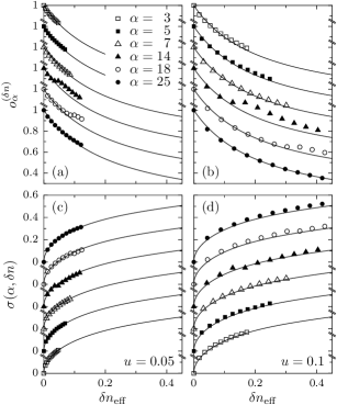
Figure 3: Same data as in Fig. 2 but as a function of $\delta n_{\mathrm{eff}}$ (Eq. (4)). The solid lines are predicted from a continuous Gaussian process with $\eta=1$. To avoid overlap, the curves are shifted with respect to each other. The agreement is quite remarkable except when an empty level becomes filled (i.e., for $\alpha=14,18$).

Gaussian random processes (GP). Our scaling equation (4) and the universal correlators can be derived from GP. Continuous GP alhassid95 depend upon an external parameter $x$ and are known to describe non–interacting chaotic or diffusive systems which, upon rescaling $x$, display universal parametric level correlations simons93 . For small values of $|x-x^{\prime}|$, the random Hamiltonian $h_{jk}(x)$ with orthogonal symmetry obeys

$$\overline{h_{ij}(x)h_{kl}(x^{\prime})}\propto(\delta_{ik}\delta_{jl}+\delta_{il}\delta_{jk})[1-\kappa|x-x^{\prime}|^{\eta}+\ldots]\text{ }.$$ (5)

This defines the continuous GP with exponent $\eta$ attias95 . The usual parametric random–matrix models discussed in the literature are differentiable GP for which $\eta=2$. In contradistinction, we will show that in the HF approximation, the addition of electrons corresponds to a GP with $\eta=1$. This exponent is characteristic of Brownian motion (where time plays the role of the parameter $x$).

Generalized Koopmans’ approach. To understand the universality of scrambling we use a generalized Koopmans’ approach. With $\alpha$ denoting the single-particle eigenstates of the $n$–electron HF Hamiltonian, that Hamiltonian is given by

$$h_{\alpha\gamma}^{(n)}=h_{\alpha\gamma}^{(0)}+\sum_{\beta=1}^{n}v_{\alpha\beta;\gamma\beta}^{A}=\delta_{\alpha\gamma}\epsilon_{\alpha}^{(n)}$$ (6)

where the sum is over the lowest $n$ levels. In the same basis, the HF Hamiltonian for $(n+1)$ electrons is

$$h_{\alpha\gamma}^{(n+1)}=h_{\alpha\gamma}^{(0)}+\sum_{\beta\delta}v_{\alpha\beta;\gamma\delta}^{A}\rho_{\delta\beta}\;,$$ (7)

where $\rho_{\delta\beta}$ is the single–particle density matrix (a projector onto the lowest $(n+1)$ eigenstates of the HF problem with $(n+1)$ electrons). We expand $h_{\alpha\gamma}^{(n+1)}$ around $h_{\alpha\gamma}^{(n)}$ up to first order in $v$. Using $\rho_{\delta\beta}=\delta_{\delta\beta}\Theta(n+1-\beta)+O(v)$ and Eq. (6) we find

$$h_{\alpha\gamma}^{(n+1)}\approx h_{\alpha\gamma}^{(n)}+w_{\alpha\gamma}^{(n)}\;\;\mathrm{where}\;\;w_{\alpha\gamma}^{(n)}\equiv v_{\alpha n+1;\gamma n+1}^{A}\ .$$ (8)

The approximation leading to Eq. (8) is tantamount to ignoring the change in the HF wave functions that occurs when an electron is added to the dot. When restricted to the diagonal elements of Eq. (8), this neglect is known as Koopmans’ approximation. Hence, our Eq. (8) can be considered a generalized Koopmans’ relation.

Brownian Motion. To determine the statistical properties of the matrix $w$, we use the last Eq. (8). For small $|u|$, the interaction matrix elements in the HF basis were shown alhassid05 to be uncorrelated Gaussian random variables with variances that are very close to their input values in the basis used in Eq. (1). This implies that the $w_{\alpha\gamma}$’s are uncorrelated Gaussian random variables with mean values zero and variances $\sigma^{2}(w_{\alpha\gamma}^{(n)})=2(1+\delta_{\alpha\gamma})(1-\delta_{\alpha n+1})(1-\delta_{n+1\gamma})u^{2}$. The Kronecker symbols in the last two brackets are due to antisymmetrization and imply that the matrix $w$ carries zeros in the row and column labelled $(n+1)$. Except for this fact the matrices $w^{(n)}$ form a Gaussian orthogonal ensemble. The single–particle HF wave functions (which determine $w^{(n)}$) are not correlated with the eigenvalues $\epsilon_{\alpha}^{(n)}$. Therefore, the matrices $w^{(n)}$ and $h^{(n)}$ are uncorrelated. Thus, for small $|u|$ and except for effects of the HF gap, the set of HF Hamiltonians $h^{(n)},h^{(n+1)},\ldots$ with a discrete parameter $n$ corresponds approximately to a discrete orthogonal GP (see Ref. attias95 ). We use the fact that such a GP can be embedded into a continuous orthogonal GP $h(x)$ by the requirement that $h^{(n)}=h(x_{n})$ for a set of discrete points $x_{n}$ with equal spacings $\delta x=x_{n+1}-x_{n}$.

The exponent $\eta$ of that GP is determined by the fact that the matrices $w^{(n)}$ and $w^{(n+1)}$ are approximately uncorrelated. When we use Eq. (8) for both matrices and approximate the HF basis for $(n+1)$ electrons by that for $n$ electrons, this follows from the fact that the matrix elements $v_{\alpha n+2;\alpha n+2}^{A}$ and $v_{\alpha n+1;\alpha n+1}^{A}$ are uncorrelated in that basis. We have checked numerically that $w^{(n)}$ and $w^{(n+1)}$ remain essentially uncorrelated even when the matrix elements $v_{\alpha n+2;\alpha n+2}^{A}$ are evaluated in the HF basis of $(n+1)$ electrons. We conclude that our discrete GP is characterized by $\overline{[h(x_{n+2})-h(x_{n+1})][h(x_{n+1})-h(x_{n})]}\approx\overline{w^{(n+1)}w^{(n)}}\approx 0$. This implies that the GP must have an exponent of $\eta=1$. Indeed, for a GP satisfying Eq. (5) we have $\!\!\!\overline{[h(x_{n+2})-h(x_{n+1})][h(x_{n+1})-h(x_{n})]}\propto(2^{\eta-1}-1)(\delta x)^{\eta}.$ That correlator vanishes if and only if $\eta=1$.

The solid lines in Fig. 3 show that our approximation works even though we do not deal with a true GP ($w^{(n)}$ carries zeros in row and column $(n+1)$). To see why, we omit on the right–hand side of Eq. (8) in $h^{(n)}$ the eigenvalue $\epsilon_{n+1}^{(n)}$ and in $w^{(n)}$ row and column labelled $n+1$ and perform the step $n\rightarrow(n+1)$. This procedure is repeated with $n$ replaced by $(n+1)$, etc. We obtain a genuine GP except for the spacing of the eigenvalues $\epsilon_{\alpha}^{(n)}$. These obey Wigner–Dyson statistics for $\alpha\leq n$ and for $\alpha\geq(n+1)$ (see Ref. alhassid05 ) while the HF gap separating these two sets of levels does not. Because of the gap the process is not a GP and we expect less mixing between levels below and above the gap than would otherwise occur. We thus expect (on top of the step seen in the data) a slowing–down of the decorrelation in the vicinity of the Fermi level. It appears that this effect is too small to rise above the statistical uncertainties.

Scaling of $n$. Universal correlations are obtained by scaling the parameter $x$. The scaled parameter for a GP with exponent $\eta$ is generally given by $x_{\mathrm{eff}}=D^{1/\eta}x$ where $D=\left[\overline{(\tilde{\epsilon}_{\alpha}(x+\delta x)-\tilde{\epsilon}_{\alpha}(x))^{2}}/\delta x^{\eta}\right]$. We identify $x$ with $n$ and use that relation for the smallest possible change $\delta n=1$ to define (for $\eta=1$) the scaled parameter $n_{\mathrm{eff}}=\overline{{(\tilde{\epsilon}_{\alpha}^{(n+1)}-\tilde{\epsilon}_{\alpha}^{(n)})}^{2}}.$ Assuming that $\Delta(\epsilon_{\alpha})$ does not change much when one electron is added and using Koopmans’ limit, we estimate $\tilde{\epsilon}_{\alpha}^{(n+1)}-\tilde{\epsilon}_{\alpha}^{(n)}\approx(\epsilon_{\alpha}^{(n+1)}-\epsilon_{\alpha}^{(n)})/\Delta(\epsilon_{\alpha})\approx v_{\alpha n+1;\alpha n+1}^{A}/\Delta(\epsilon_{\alpha})$. Since $\sigma^{2}(v_{\alpha n+1;\alpha n+1}^{A})=4u^{2}$, we obtain the simple approximate scaling given in Eq. (4). In general, the mean level spacing in Eq. (4) depends (weakly) on $n$. Although $n$ is a discrete parameter, the scaled parameter $n_{\mathrm{eff}}$ can be made as close to being continuous as we like by choosing a sufficiently small $u$.

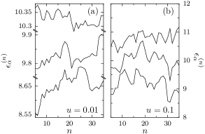
Figure 4: The addition of electrons to a quantum dot is analogous to Brownian motion. Shown are three HF single–particle levels $\epsilon_{\alpha}^{(n)}$ versus the number $n$ of electrons for $u=0.1$ (right) and $u=0.01$ (left). Notice the finer scale on the left.

Discussion. The solid lines in the top (bottom) panels of Fig. 3 display the two universal GP curves for $o(\delta x)=\overline{|\langle\psi(x+\delta x)|\psi(x)\rangle|^{2}}$ and for $\sigma(\alpha,\delta x)$. These are computed numerically from an $\eta=1$ GP whose parameter $x$ is scaled according to the prescription given in the previous paragraph and identified with $\delta n_{\mathrm{eff}}$. The wave–function correlator can be well fit by $o(\delta n_{\mathrm{eff}})\approx[1+\delta n_{\mathrm{eff}}/\alpha]^{-1}$ with $\alpha=0.23$ rmp00 . The steps in the data for $\alpha=14\ (18)$ at $\delta n=4\ (8)$ can be understood in the framework of the generalized Koopmans approximation (8). In the HF approximation of the $n$–electron dot, the level $\alpha=(n+1)$ is empty. In the approximation (8) this level is not coupled by the perturbation $w^{(n)}$ to any other HF eigenstate $\gamma$ (we recall that $w_{\gamma,n+1}^{(n)}=w_{n+1,\gamma}^{(n)}=0$) and is, therefore, also an eigenstate of $h^{(n+1)}$. In particular, $\epsilon_{\alpha=n+1}^{(n+1)}\approx\epsilon_{\alpha=n+1}^{(n)}$ and $\psi_{\alpha=n+1}^{(n)}\approx\psi_{\alpha=n+1}^{(n+1)}$. This is why the measures for both spectral and wave–function scrambling remain approximately unchanged between $n=\alpha-1$ and $n=\alpha$.

When plotted versus $n$, the single–particle HF levels should exhibit Brownian–motion–like behavior since the addition of electrons is an $\eta=1$ GP even for very small $u$. This is verified in Fig. 4 where we show three HF levels versus $n$ for a particular realization of the induced ensemble. When $u$ is reduced from $u=0.1$ (right) to $u=0.01$ (left), the behavior remains non–analytic although on a much finer scale.

In conclusion, we have shown that, in a chaotic or diffusive dot with interactions, the scrambling of HF levels due to the addition of electrons is described by a Brownian–motion type process. The change of the number $n$ of electrons is analogous to a discrete equally–spaced time series. We have used a non–universal scaling of $n\rightarrow n_{\mathrm{eff}}$ to show that the measures of scrambling of both HF levels and HF wave functions versus $n_{\mathrm{eff}}$ follow closely the corresponding universal correlators of an $\eta=1$ Gaussian random process. The only exception occurs when an empty level becomes filled, causing a delay in the scrambling process by one electron.

This work was supported in part by the U.S. DOE grant No. DE-FG-0291-ER-40608. We thank Y. Gefen and Ph. Jacquod for useful discussions. Y.A. acknowledges support by a von Humboldt Senior Scientist Award and the hospitality of the Max-Planck-Institut für Kernphysik at Heidelberg where part of this work was completed.

References

- (1) T. Guhr, A. Müller-Groeling, and H. A. Weidenmüller, Phys. Rep. 299, 190 (1998).
- (2) Y. Alhassid, Rev. Mod. Phys. 72, 895 (2000).
- (3) S.R. Patel et al., Phys. Rev. Lett. 81, 5900 (1998).
- (4) Y. Alhassid and Y. Gefen, cond-mat/0101461.
- (5) Ya. M. Blanter, A.D. Mirlin, and B.A. Muzykantskii, Phys. Rev. Lett. 78, 2449 (1997).
- (6) T. Koopmans, Physica (Amsterdam) 1, 104 (1934).
- (7) Y. Alhassid and H. Attias, Phys. Rev. Lett. 74, 4635 (1995).
- (8) Y. Alhassid, H.A. Weidenmüller, and A. Wobst, Phys. Rev. B 72, 045318 (2005).
- (9) B.D. Simons and B.L. Altshuler, Phys. Rev. Lett. 70, 4063 (1993); Phys. Rev. B 48, 5422 (1993).
- (10) H. Attias and Y. Alhassid, Phys. Rev. E 52, 4776 (1995).