On elliptical soft colloids in smectic-$C$ films

Abstract

We investigate theoretically the elliptical shapes of soft colloids in freely standing smectic C films, that have been reported recently. The colloids favour parallel alignment of the liquid crystal molecules at their surfaces and, for sufficiently strong anchoring, will generate a pair of defects at the poles of the colloidal particles. The elastic free energy of the liquid crystal matrix will, in turn, affect the shape of the colloids. In this study we will focus on elliptical soft colloids and determine how their equilibrium shapes depend on the elastic constants of the liquid crystal, the anchoring strength, the surface tension and the size of the colloids. A shape diagram is obtained analytically, by minimizing the Frank elastic free energy, in the limit of small eccentricities. The analytical results are verified, and generalized to arbitrary eccentricities, by numerical minimization of an appropriate Landau free energy. The latter is required for an adequate description of the topological defects when the liquid crystal correlation length is comparable to the size of the colloidal particles.

I Introduction

Owing to their intriguing and complex behaviour, colloidal dispersions in liquid crystals have been the subject of numerous studies in recent years Stark.2001 . The behaviour of these inverted emulsions depends upon (i) the elastic constants of the liquid crystal, (ii) the size and shape of the colloidal particles, (iii) the surface tension and (iv) the boundary conditions at the surface of the container. These contributions lead to highly anisotropic long-ranged colloidal interactions Poulin.Weitz.1998 ; Tasinkevych.etal.2002 that result in a variety of self-organised colloidal structures, such as linear chains Poulin.etal.1997 ; Loudet.etal.2000 ; Cluzeau.etal.2001 ; Cluzeau1.etal.2002 ; Voltz.Stannarius.2004 , periodic lattices Voltz.Stannarius.2004 ; Nazarenko.etal.2001 ; Cluzeau2.etal.2002 , anisotropic clusters Poulin.etal.1999 , and cellular structures Meeker.etal.2000 stabilized, in general, by the presence of topological defects.

The competition of elastic and surface energies may also determine the shape of nematic droplets Chandrasekhar.1965 ; Huang.Tuthill.1994 . Indeed, for sufficiently large parallel anchoring, nematic droplets were found to exhibit sharp ends Virga.1994 . These shapes are known as tactoids and the tactoidal shape is more pronounced for smaller droplets. As the size of the droplet increases, the contribution of the isotropic surface tension also increases and, as a result, the shape of the droplets becomes spheroidal Prinsen.Schoot.2003 . Recent studies on the shape of isotropic soft colloids in a nematic liquid crystal illustrate this behaviour and reveal a way of controlling the shape of the droplets using surfactants Lishchuk.Care.2004 .

Freely standing smectic films (Sm FSF’s) are two-dimensional systems obtained by spreading a smectic liquid crystal through a hole drilled into a substrate. These films are useful systems to study surface interactions, effects of reduced dimensionality on liquid crystal phase transitions Winkle.Clark.1988 , and interactions between soft colloids Cluzeau.etal.2001 ; Cluzeau1.etal.2002 ; Voltz.Stannarius.2004 ; Patricio.etal.2002 . Soft colloids or inclusions are created by (i) rapid reduction of the film area, (ii) blowing across the film to pull material from the meniscus region or (iii) heating the system near the smectic-to-isotropic or smectic-to-nematic phase transition Pettey.etal.1998 .

The thickness of Sm FSF’s ranges from a few thousand down to two smectic layers. Recent studies on Sm-$C^{*}$ FSFs at the Sm-$C^{*}$-cholesteric ($N^{*}$) phase transition, revealed the existence of an intermediate thickness where $N^{*}$ soft colloids are nucleated Cluzeau.etal.2003 . For thin films (${\cal N}<24$; ${\cal N}$ is the number of layers) the phase transition is driven by layer-by-layer thinning, while for thick films (${\cal N}>400$) the $N^{*}$ order is stabilised and appears through the nucleation of $N^{*}$ fingers.

Experimental studies on the ordering of soft colloids in Sm-$C^{*}$ FSF report that the molecules in the liquid crystal matrix are aligned perpendicular to the colloidal surfaces, nucleating one hyperbolic topological defect close to the colloidal surfaces Cluzeau.etal.2001 . By contrast, experiments on Sm-$C$ FSF report that the liquid crystal molecules are aligned parallel to the colloidal surfaces Cluzeau1.etal.2002 ; Voltz.Stannarius.2004 ; Cluzeau2.etal.2002 . Under these conditions, a pair of defects may be nucleated at the poles of the colloidal particles which, in turn, affect the colloidal shape as reported by Cluzeau et al Cluzeau1.etal.2002 . Large colloids are found to be almost circular, while smaller ones are elliptical, with the long axis oriented along the Sm-$C$ director, ${\bf c}$.

Here we carry out a theoretical investigation of the shape of soft colloids. We restrict our study to the elliptical shapes observed in the experiment referred to above Cluzeau1.etal.2002 and will not consider tactoids. This article is organized as follows. In section II we describe the Frank free energy for Sm-$C$ FSF’s. In Section III, we calculate analytically the configuration of the ${\bf c}$-director for elliptical soft colloids, in the limit of small eccentricities. These results provide a complete (albeit approximate) description of the dependence of the equilibrium shape (optimal eccentricity) on material parameters, that will be used to guide the subsequent numerical study. In Section IV we use a Landau free energy to investigate numerically the same problem and compare the results obtained using both approaches. Finally, in Section V we summarize our conclusions.

II Free energy

The free energy of a Sm FSF takes into account the deformations of the in-layer molecular alignment, or orientational order, represented by a two dimensional vector field ${\bf c}=(\cos\theta,\sin\theta)$. It is given by

$${\cal F}= \frac{1}{2} \int_{\Omega}d{\it S}\left[{\cal K}_{s}(\mbox{\boldmath$\nabla$}\cdot{\bf c})^{2}+{\cal K}_{b}(\mbox{\boldmath$\nabla$}\times{\bf c})^{2}\right]$$ (1)

$$+ \int_{\partial\Omega}d{\it l}\left(\gamma+\frac{\cal W}{2}\sin{{}^{2}(\theta^{s}-\theta)}\right),$$

where ${\cal K}_{s}$ and ${\cal K}_{b}$ are the splay and bend elastic constants, and $\gamma$ and ${\cal W}$ are the isotropic and anisotropic line tensions, respectively. $\theta^{s}$ is the preferred orientation at the boundary $\partial\Omega$. In general, ${\cal K}_{s}$ and ${\cal K}_{b}$ are different but, for simplicity, we will use the one-elastic constant approximation, ${\cal K}_{s}={\cal K}_{b}={\cal K}$. The bulk elastic free energy density is then given by ${\cal K}(\mbox{\boldmath$\nabla$}\theta)^{2}/2$.

Minimization of Eq.(1) with respect to $\theta(x,y)$ yields

$$\mbox{\boldmath{$\nabla$}}^{2}\theta = 0\qquad\mbox{in $\Omega$, }$$ (2)

$$\mbox{\boldmath{$\nu$}}\cdot\mbox{\boldmath{$\nabla$}}\theta-\frac{{\cal W}}{2{\cal K}}\sin{2(\theta^{s}-\theta)} = 0\qquad\mbox{in $\partial\Omega$, }$$ (3)

where $\nu$ is the unit vector normal to the boundary $\partial\Omega$.

III Elliptic deformations

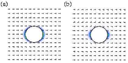
Figure 1: (Color online) Soft colloids in a smectic-$C$ layer with correlation length $\xi=0.1{\cal R}$. The vectors represent the ${\bf c}$-director, while the colored regions correspond to strong variations of the order parameter and signal the surface defects. (a) $\omega={\cal WR}/{\cal K}=1.0$, $\sigma=\gamma{\cal R}/{\cal K}=10$ and optimal eccentricity $e^{*}=0.270$. (b) $\omega=10$, $\sigma=100$ and $e^{*}=0.127$.

Let us consider a soft colloid in a smectic layer (Fig. (1)). The shape of the colloid is not fixed but depends, in particular, on the line tension. If the isotropic line tension is large, the colloid is circular, or slightly distorted. For simplicity, we start by considering elliptical deformations with small eccentricities.

The problem of finding the equilibrium shape, or the optimal eccentricity, is simplified by using elliptic coordinates

$$\left\{\begin{array}[]{ll}x&={\cal R}_{e}\cosh{u}\cos{\phi},\\ y&={\cal R}_{e}\sinh{u}\sin{\phi}.\end{array}\right.$$ (4)

where ${\cal R}_{e}=e{\cal R}(1-e^{2})^{-1/4}$, the eccentricity of the colloid is $e=1/\cosh{u^{s}}$ and $u^{s}$ is the minimal value of $u$, at the boundary of the colloid. ${\cal R}=\sqrt{A/\pi}$, where $A$ is the area of the soft colloid.

In what follows we assume that the colloidal boundary favours a parallel orientation of the in-plane liquid crystal director. This will depend on the eccentricity of the colloid and is given by

$${\theta}^{s}=-\arctan{\left[\sqrt{1-e^{2}}\frac{\sin{2\phi}}{1-\cos{2\phi}}\right]}.$$ (5)

The solution of the Laplace equation(2) is straightforward and has the general form

$$\theta(u,\phi)=\sum_{m=0}^{\infty}\exp{\{-mu\}}\left({\cal U}_{m}\sin{m\phi}+{\cal V}_{m}\cos{m\phi}\right),$$ (6)

for uniform liquid crystal alignment at infinity. Note that $\theta(u,\phi)$ satisfies the following symmetries: $(i)$ $\theta(u,-\phi)=-\theta(u,\phi)$ and $(ii)$ $\theta(u,\pi-\phi)=-\theta(u,\phi)$, implying that ${\cal V}_{m}=0$ and restricting the nonzero coefficients to those with even indices, respectively. Redefining the coefficients ${\cal U}_{2m}\rightarrow{\cal U}_{2m}\exp\{2mu^{s}\}$, we write

$$\theta(u,\phi)=\sum_{m=1}^{\infty}{{\cal U}}_{2m}\exp\{-2m(u-u^{s})\}\sin{2m\phi}.$$ (7)

The analytical solution for elliptical soft colloids, for $e\ll 1$, is obtained using perturbation theory. We expand the coefficients ${\cal U}_{2m}={\cal U}_{2m}^{(0)}+e^{2}{\cal U}_{2m}^{(2)}+e^{4}{\cal U}_{2m}^{(4)}+...$, of the solution $\theta=\theta_{0}+e^{2}\theta_{2}+e^{4}\theta_{4}+...$, and generalize the method used for circular colloids in Burylov.Raikher . Assuming that ${\cal U}_{2m}^{(0)}=-p_{0}^{m}/m$, for circular soft colloids, $\theta_{0}$, is given by

$$\theta_{0}=-\arctan{\left[\frac{p_{0}\exp{\{-2(u-u^{s})\}}\sin{2\phi}}{1-p_{0}\exp{\{-2(u-u^{s})\}}\cos{2\phi}}\right]}.$$ (8)

where $p_{0}$ is obtained by minimizing the free energy Eq.(1). This yields a second order algebraic equation

$$p_{0}^{2}+(4/\omega)p_{0}-1=0,$$ (9)

with a positive root $p_{0}=(2/\omega)\left[\sqrt{1+(\omega/2)^{2}}-1\right]$, where $\omega={\cal W}{\cal R}/{\cal K}$ is a dimensionless ratio of the anchoring and elastic strengths.

Suppose we can write the free energy density as $f[\theta]=f_{0}[\theta]+e^{2}f_{2}[\theta]+e^{4}f_{4}[\theta]+...$ A functional Taylor expansion of the free energy about the solution for a circular colloid, $\theta_{0}$, yields

$${\cal F}[\theta]=\int{d^{2}{\bf x}(f_{0}[\theta_{0}]+e^{2}f_{2}[\theta_{0}]+e^{4}f_{4}[\theta_{0}])}+$$

$$\int{d^{2}{\bf x}\Delta\theta({\bf x})\left(\left.\frac{\delta f_{0}}{\delta\theta({\bf x})}\right|_{\theta_{0}}+e^{2}\left.\frac{\delta f_{2}}{\delta\theta({\bf x})}\right|_{\theta_{0}}\right)}+$$

$$\frac{1}{2}\int{d^{2}{\bf x}^{\prime}\int{d^{2}{\bf x}\Delta\theta({\bf x})\left.\frac{\delta^{2}f_{0}}{\delta\theta({\bf x})\delta\theta({\bf x}^{\prime})}\right|_{\theta_{0}}\Delta\theta({\bf x}^{\prime})}}+...,$$ (10)

where $\Delta\theta=\theta-\theta_{0}=e^{2}\theta_{2}+e^{4}\theta_{4}+...$, and the expansion is valid to the fourth order in the eccentricity. This is simplified using the equilibrium condition for the circular case, $\left.\delta f_{0}/\delta\theta\right|_{\theta_{0}}=0$, which implies that $\theta_{2}$ and $\theta_{4}$ are not present in the terms of order $e^{2}$ and $e^{4}$, respectively, yielding for the free energy

$${\cal F}[\theta]={\cal F}_{0}[\theta_{0}]+e^{2}{\cal F}_{2}[\theta_{0}]+e^{4}{\cal F}_{4}[\theta_{0},\theta_{2}]+...$$ (11)

The transition from circular to elliptical shape is controlled by the sign of ${\cal F}_{2}$, which depends only on $\theta_{0}$. If this term is positive, the soft colloid is circular; otherwise it is elliptical. To determine the optimal eccentricity, we begin by minimizing the free energy (Eq.(11)) with respect to $\theta_{2}$. The solution satisfies the linear equation $\delta{\cal F}_{4}/\delta\theta_{2}=0$, and may be written as

$$\theta_{2}({\bf x})=-\int{d^{2}{\bf x^{\prime}}\left[\left.\frac{\delta^{2}f_{0}}{\delta\theta({\bf x})\delta\theta({\bf x^{\prime}})}\right|_{\theta_{0}}\right]^{-1}}\left.\frac{\delta f_{2}}{\delta\theta({\bf x^{\prime}})}\right|_{\theta_{0}}$$ (12)

The general solution $\theta$ is a linear combination of the solutions of the Laplace equation, in terms of which the linear equation becomes a matrix equation for the set of coefficients ${\cal U}_{2m}^{(2)}$, and Eq. (12) an (infinite) matrix inversion. The optimal eccentricity is then, $e^{*}=\sqrt{-{\cal F}_{2}[\theta_{0}]/2{\cal F}_{4}[\theta_{0},\theta_{2}]}$.

In order to determine ${\cal F}_{0}$, ${\cal F}_{2}$ and ${\cal F}_{4}$ in Eq. (11), we proceed by noting that the bulk elastic free energy may be integrated by parts, yielding

$${\cal F}_{\cal K}/{\cal K}= - \frac{1}{2}\int_{0}^{2\pi}d\phi\theta\left.\frac{\partial\theta}{\partial u}\right|_{\partial\Omega}$$

$$\simeq - {\cal E}_{0}[p_{0}]-e^{4}\int_{0}^{2\pi}d\phi\frac{\theta_{2}}{2}\left.\frac{\partial\theta_{2}}{\partial u}\right|_{\partial\Omega},$$ (13)

where $-{\cal KE}_{0}[p_{0}]=-\pi{\cal K}\log{(1-p_{0}^{2})}$ is the elastic free energy of a circular soft colloid. Terms of order $e^{2}$ and $e^{4}$, that depend on $\theta_{2}$ and $\theta_{4}$ respectively, were neglected since they do not contribute to the total free energy.

The term corresponding to the isotropic line tension $\gamma$ is independent of $\theta$. Its expansion in the eccentricity yields

$${\cal F}_{\gamma}/{\cal K}=\gamma/{\cal K}\int_{\partial\Omega}dl\simeq 2\pi\sigma\left(1+\frac{3}{64}e^{4}\right).$$ (14)

where we used $dl/d\phi={\cal R}_{e}\sqrt{1-e^{2}\cos^{2}\phi}/e$. $\sigma=\gamma{\cal R}/{\cal K}$ is the ratio of the isotropic line tension and the elastic strength.

The expansion of the contribution of the anisotropic line tension or anchoring strength, ${\cal W}$, is obtained by expanding the preferred orientation (Eq.(5)), $\theta^{s}=\theta_{0}^{s}+e^{2}\theta_{2}^{s}+...$ After some tedious algebraic and trigonometric manipulations, we obtain

$${\cal F}_{\cal W}/{\cal K} = \frac{\cal W/K}{2}\int_{\partial\Omega}d{\it l}\sin{{}^{2}\left(\theta^{s}-\theta\right)}$$ (15)

$$\simeq \frac{\omega}{2}\left[{\cal S}_{0}[p_{0}]+e^{2}{\cal S}_{2}[p_{0}]+e^{4}\bigg{\{}{\cal S}_{4}[p_{0}]\right.$$

$$+ \int_{0}^{2\pi}d\phi\theta_{2}\big{(}\theta_{2}-2\theta_{2}^{s}\big{)}\cos{2\big{(}\theta_{0}^{s}-\theta_{0}\big{)}}$$

$$+ \left.\int_{0}^{2\pi}d\phi\frac{\theta_{2}}{4}\cos{2\phi}\sin{2\big{(}\theta_{0}^{s}-\theta_{0}\big{)}}\bigg{\}}\right].\qquad$$

where ${\cal K}\omega{\cal S}_{0}[p_{0}]/2=\pi{\cal K}\omega(1-p_{0})/2$ is the anchoring energy for a circular soft colloid, ${\cal S}_{2}[p_{0}]=-3\pi(1-p_{0}^{2})/8$ and ${\cal S}_{4}[p_{0}]=\pi(-18+5p_{0}+24p_{0}^{2}-3p_{0}^{3})/128$.

By adding Eqs.(13), (14) and (15) we obtain the free energy, ${\cal F}[\theta]\simeq{\cal F}_{0}[p_{0}]+e^{2}{\cal F}_{2}[p_{0}]+e^{4}{\cal F}_{4}[p_{0},\theta_{2}]$, where

$${\cal F}_{0}[p_{0}]/{\cal K} = -{\cal E}_{0}[p0]+2\pi\sigma+\omega{\cal S}_{0}[p_{0}]/2,$$ (16)

$${\cal F}_{2}[p_{0}]/{\cal K} = \omega{\cal S}_{2}[p_{0}]/2$$ (17)

and

$${\cal F}_{4}[p_{0},\theta_{2}]/{\cal K} = \frac{\omega}{2}{\cal S}_{4}[p_{0}]+\frac{3}{32}\pi\sigma-\frac{1}{2}\int_{0}^{2\pi}d\phi\theta_{2}\left.\frac{\partial\theta_{2}}{\partial u}\right|_{\partial\Omega}$$ (18)

$$+ \frac{\omega}{2}\int_{0}^{2\pi}d\phi\theta_{2}(\theta_{2}-2\theta_{2}^{s})\cos{2(\theta_{0}^{s}-\theta_{0})}$$

$$+ \frac{\omega}{8}\int_{0}^{2\pi}d\phi\theta_{2}\cos{2\phi}\sin{2(\theta_{0}^{s}-\theta_{0})}.$$

Inspection of ${\cal F}_{2}[p_{0}]$ reveals that the shape transition is controlled by the dimensionless quantity, $\omega$. It is clear, from the definition of $p_{0}$, that ${\cal F}_{2}$ is negative for any finite value of $\omega$ and thus the equilibrium shape is elliptical, except when $\omega$ vanishes (weak anchoring).

In order to calculate $\theta_{2}$, we approximate the general solution by a finite number of terms in (7), corresponding to a small number of coefficients ${\cal U}_{2m}^{(2)}$. Explicit calculations reveal that the first two coefficients, ${\cal U}_{2}^{(2)}$ and ${\cal U}_{4}^{(2)}$, are sufficient to yield $\theta_{2}$ and the eccentricity $e^{*}$ with an accuracy better than $1\%$ and $0.6\%$, respectively.

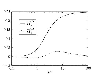
Figure 2: ${\cal U}_{2}^{(2)}$ and ${\cal U}_{4}^{(2)}$ as functions of the reduced anchoring strength $\omega={\cal WR/K}$. Higher order coefficients lead to small corrections (less than $0.6\%$) to the optimal eccentricity $e^{*}$.

Figure (2) illustrates the dependence of ${\cal U}_{2}^{(2)}$ and ${\cal U}_{4}^{(2)}$ on the reduced anchoring strength $\omega$. For weak anchoring, as $\omega$ vanishes, we find

$$\left\{\begin{array}[]{ll}{\cal U}_{2}^{(2)}&=\frac{13}{256}\omega^{2}\\ \\ {\cal U}_{4}^{(2)}&=-\frac{\omega}{64}\end{array}\right.\qquad(\omega\ll 1).$$ (19)

while for strong anchoring,

$$\left\{\begin{array}[]{ll}{\cal U}_{2}^{(2)}&=\frac{1}{4}\left(1-\frac{1}{\omega}\right)-\frac{1}{2\omega^{2}}\\ \\ {\cal U}_{4}^{(2)}&=\frac{1}{2\omega}-\left(\frac{2}{\omega}\right)^{2}\end{array}\right.\qquad(\omega\gg 1).$$ (20)

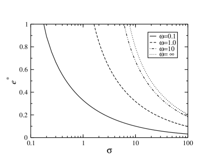
Figure 3: Optimal eccentricity $e^{*}$ as a function of $\sigma=\gamma{\cal R/K}$, at fixed values of $\omega={\cal WR/K}=0.1$, $1.0$, $10$, $\infty$.

In Fig. (3) we plot the optimal eccentricity $e^{*}$ as a function of $\sigma$, at fixed values of $\omega=0.1$, $1.0$, $10$, $\infty$. As expected, the stability of the elliptical shape decreases as $\sigma$ increases. We note, however, that the rate at which the eccentricity $e^{*}$ decreases as $\sigma$ increases depends on $\omega$. In fact, as $\omega$ increases a larger isotropic tension, $\sigma$, is required to reduce the eccentricity. In the limit of strong anchoring, the liquid crystal molecules are parallel to the surface of the soft colloid, but at the same time, are parallel to each other, to minimize the elastic free energy. These conditions imply a strong eccentricity, or a pronounced elliptical shape, of the soft colloid. The isotropic line tension, on the other hand, favours circular soft colloids, minimizing the perimeter and reducing the eccentricity.

For weak anchoring, the optimal eccentricity has the asymptotic behaviour

$$e^{*}\simeq(\omega/\sigma)^{1/2}+3/8(\omega/\sigma)^{3/2}\qquad(\omega\ll 1).$$ (21)

This expansion clearly reveals a bifurcation at $\omega=0$. At zero anchoring, the liquid crystal is not aligned by the colloidal boundary, and the shape of the soft colloid is circular. For positive values of $\omega$, the soft colloid becomes elliptical. For strong anchoring, the optimal eccentricity ,$e^{*}$, has the asymptotic behaviour

$$e^{*}\simeq\frac{2}{\sqrt{\sigma-11/3}}-\frac{\sqrt{3}(19+12\sigma)}{2(3\sigma-11)^{3/2}}\frac{1}{\omega}\qquad(\omega\gg 1).$$ (22)

When $\omega\to\infty$ the colloidal shape is strongly affected by the elastic deformation of the liquid crystal matrix and the eccentricity is determined by the competition between the isotropic line tension and the elastic free energy. When $\sigma$ is large, the eccentricity is small, and the soft colloid is almost circular. As $\sigma$ decreases, the soft colloid becomes more elliptical and, eventually, this perturbation theory breaks down. We note, however, that the absence of solutions of (22) for $\sigma<11/3$ may indicate the stability of other colloidal shapes, such as the tactoid, an elongated shape with two singularities or cusps at its extremities.

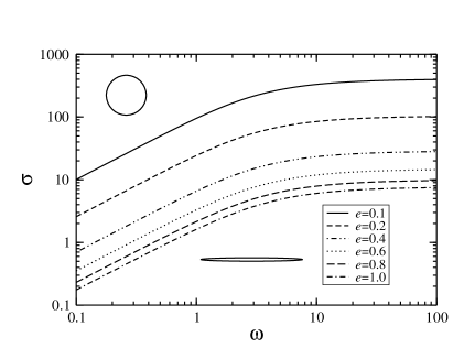
Figure 4: Shape diagram: lines of constant eccentricity in the $\omega$-$\sigma$ plane. The circle and the ellipse schematically shown occur for $e=0$ and $e=0.9$, respectively.

Figure (4) illustrates the shape “diagram” of the soft colloid depicting lines of constant eccentricity in the $\omega$-$\sigma$ plane. These curves exhibit two regimes. For $\omega<1$, the slope of the constant eccentricity lines indicates that $\sigma$ is proportional to $\omega$. For larger values of $\omega$, however, the lines are nearly flat, indicating a dependence on $\sigma$ only. The lower line on the diagram corresponds to a “critical” value of $\sigma_{c}$ where the eccentricity of the colloid is $e^{*}=1$ and the elliptical shape becomes unstable.

The shape diagram reveals that colloids with approximately circular shapes ($e\to 0$) occur when $\sigma$ is 2-3 orders of magnitude larger than $\omega$, in the weak anchoring regime. In the strong anchoring regime, nearly circular colloids occur at large values of $\sigma$ with a dependence on $\omega$ that is less marked. This means that the shape of the colloids depends not only on the ratio of the isotropic to anisotropic line tensions $\sigma/\omega$, but also on the director configuration, as expected.

IV Numerical solutions

The Frank elastic free energy used in the previous section (Eq. (1)) describes the general features of soft colloids in liquid crystals. However, it does not describe adequately the topological defects that may occur in the strong anchoring regime. The structure of these defects is relevant for colloids with sizes comparable to the liquid crystal correlation length. Furthermore, the analytical solutions described above are based on a perturbation theory that is valid for small eccentricities only.

For completeness, we consider a Landau-like free energy, where the orientational order parameter of the Sm-$C$ phase, $\psi=|\psi|\exp{(i\theta)}$, includes both the tilt angle $|\psi|$ and the azimuthal orientation $\theta$. The Landau free energy may be understood as a Taylor expansion in terms of the invariants of $\psi$ and of its deformations or spatial derivatives $\partial_{i}\psi$. For an isotropic Sm-$C$ film (with no preferred orientation within the layers), there is a single quadratic and a single quartic invariant of $\psi$. In what concerns the derivatives of $\psi$, however, several quadratic invariants exist but they are reduced to a single term proportional to $|\nabla\psi|^{2}=|\partial_{x}\psi|^{2}+|\partial_{y}\psi|^{2}$, in the one-elastic constant approximation.

We use this notation to rewrite the surface free energy, Eq.(1), denoting by $\psi^{s}$ the preferred order parameter at the boundary of the colloid. The surface free energy written in terms of an order parameter such as $\psi$ has to account for ($i$) the coupling between the orientation of the smectic molecules and the surface and ($ii$) the coupling between the tilt angle $|\psi|$ and the one imposed by the surface $|\psi^{s}|$, resulting in a form that is slightly different form that of Eq.(1). The total free energy is

$${\cal F}=\int_{\Omega}dS\left[-\frac{{\cal A}}{2}|\psi|^{2}+\frac{{\cal B}}{4}|\psi|^{4}+\frac{{\cal L}}{2}|\nabla\psi|^{2}\right]$$

$$+\int_{\partial\Omega}dl\left[\gamma+\frac{{\cal W}}{2}\bigg{(}1-Re\Big{\{}\frac{\psi^{s}\psi^{*}}{|\psi^{s}|^{2}}\Big{\}}^{2}\bigg{)}\right].$$ (23)

where $Re\{\}$ denotes the real part and $\psi^{*}$ is the complex conjugate of $\psi$. Using $\psi_{bulk}=\sqrt{{\cal A/B}}$, for the order parameter of the uniform Sm-$C$, and making the transformations $\tilde{\psi}=\psi/(\sqrt{2}|\psi_{bulk}|)$, $\tilde{\bf x}={\bf x}/{\cal R}$, we obtain the reduced free energy $\tilde{\cal F}={\cal F}/({\cal AR}^{2}|\psi_{bulk}|^{2})$

$$\tilde{\cal F}=\int_{\Omega}d\tilde{S}\left[|\tilde{\psi}|^{2}(|\tilde{\psi}|^{2}-1)+\varepsilon|\nabla\tilde{\psi}|^{2}\right]$$

$$+\int_{\partial\Omega}d\tilde{l}\left[\sigma+\frac{\omega}{2}\bigg{(}1-Re\Big{\{}\frac{\tilde{\psi}^{s}\tilde{\psi}^{*}}{|\tilde{\psi}^{s}|^{2}}\Big{\}}^{2}\bigg{)}\right]\varepsilon,$$ (24)

where $\varepsilon=(\xi/R)^{2}$ and $\xi=\sqrt{{\cal L/A}}=\sqrt{{\cal K/A}}/|\psi_{bulk}|$ is the correlation length of the Sm-$C$, the typical length of a defect. The Frank free energy (Eq. (1)), is recovered when $\varepsilon\to 0$. For simplicity, we have considered $|\psi^{s}|=|\psi_{bulk}|$.

The size of the colloids may be 10 to 100 times the size of the defects, i.e., $\varepsilon\ll 1$. The major difficulty in the numerical solution stems exactly from these different length scales. We use finite elements with adaptive meshing, as described in Ref.Patricio.etal.2002 , to minimize Eq.(24). A first triangulation respecting the predefined boundaries is constructed. The order parameter $\psi$ is given at the vertices of the mesh and linearly interpolated within each triangle. The free energy is then minimized using standard methods. The variation of the solution at each iteration is used to generate a new mesh. In typical calculations convergence is obtained after two mesh adaptations, corresponding to final meshes with $10^{4}$ points, spanning a region of $30{\cal R}\times 30{\cal R}$, and minimal mesh sizes of $10^{-5}{\cal R}$, close to the defects. The free energy is obtained with a relative accuracy of $10^{-3}\%$.

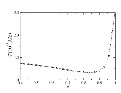
Figure 5: Reduced free energy $\tilde{\cal F}$ as a function of the eccentricity for $\varepsilon=10^{-4}$, $\omega=10$ and $\sigma=6$.

The optimal eccentricity is obtained as follows. We start by fixing the set of material parameters $\{\varepsilon$, $\omega$, $\sigma\}$. For a given value of the eccentricity $e$ the free energy of Eq.(24) is minimized. The eccentricity is incremented by $\delta e$ and the minimization is repeated. The free energy profile, as a function of $e$, exhibits a well defined minimum (in most cases), allowing the calculation of the optimal eccentricity $e^{*}$(Fig. (5)). For the smallest eccentricities $e^{*}$, however, the variation of the free energy near the minimum ${\cal F}(e^{*})$ is of the order of the relative numerical accuracy. This renders the method less accurate in the limit of circular colloids (see Fig. (7)). After determining $e^{*}$, the parameter $\sigma$ is incremented and the free energy profile is calculated.

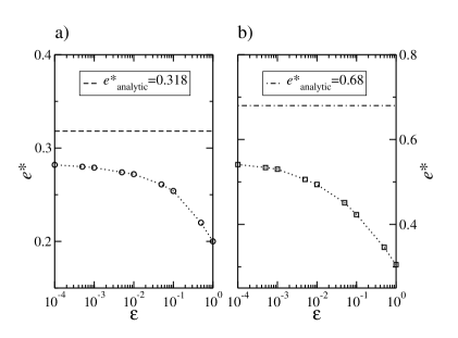
Figure 6: Optimal eccentricities as a function of $\varepsilon$ for a) $\omega=1$ and b) $\omega=10$, and $\sigma=10$

In the previous section we calculated the optimal eccentricity, $e^{*}$, analytically. Since the results are based on perturbation theory, the numerical results are not expected to match the analytical ones in the limit $\varepsilon\to 0$, for any value of $e^{*}$. Figure (6) illustrates how the optimal eccentricity depends on $\varepsilon$ for a) $\omega=1$ and b) $\omega=10$, and $\sigma=10$. Both curves approach a constant value of $e^{*}$, as $\varepsilon\rightarrow 0$ and the numerical results approach the analytical values, when $\varepsilon\rightarrow 0$, for small eccentricities.

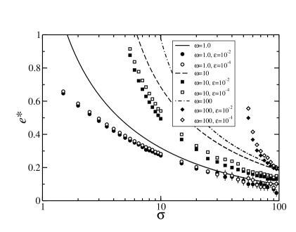
Figure 7: Optimal eccentricity $e^{*}$ as a function of $\sigma$ at constant $\omega=1$, $10$, $100$ and $\varepsilon=10^{-2}$, $10^{-4}$. Lines and symbols represent the analytical and numerical results, respectively.

In Fig. (7) we plot the numerical results together with the analytical curves for the optimal eccentricity as a function of $\sigma$, at constant $\omega=1$, $10$, $100$ and $\varepsilon=10^{-2}$, $10^{-4}$. The numerical results confirm that the optimal eccentricity is a strictly decreasing function of the line tension $\sigma$. Moreover, the decrease in the slope of $e^{*}$ versus $\sigma$ is more pronounced in the presence of surface defects ($\omega>10$). This slope does not change significantly with $\varepsilon$ (at constant $\omega$).

The numerical results for $\omega=100$ cross the corresponding analytical curve, which in view of the results for lower $\omega$, may seem surprising. This crossover was observed for anchoring strengths, in the range $10<\omega<100$, and is due to the fact that the critical value $\sigma_{c}$, where the elliptical shape becomes unstable, ($e^{*}\to 1$), does not behave as predicted by the analytical theory. In fact, while the analytical approach predicts that $\sigma_{c}/\omega$ varies considerably, the numerical results suggest a nearly constant value, $\sigma_{c}/\omega=0.505\pm 0.005$. It is likely, however, that this limit will not be observed in experiments since for most materials $\sigma/\omega\gg 1$ vanderSchoot .

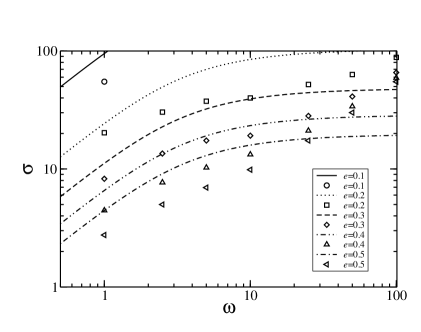
Figure 8: Shape diagram. Lines and symbols denote equilibrium shapes at constant eccentricity, in the $\omega-\sigma$ plane. The lines were obtained analytically while the symbols are the result of a numerical minimization, for systems with $\varepsilon=10^{-2}$.

In Fig. (8) we plot the numerical and the analytical shape diagrams for several values of the eccentricity ($e=0.1$,$0.2$, $0.3$, $0.4$, $0.5$). The numerical shape diagram was obtained for $\varepsilon=10^{-2}$. Results for $\varepsilon=10^{-4}$ yield similar curves, that are shifted by a small positive value of $\sigma$. The results of the numerical calculations reveal the existence of two distinct regimes. For weak anchoring, $\omega<10$, circular colloids may occur if $\sigma$ is $2$-$3$ orders of magnitude larger than $\omega$, in line with the analytical results. For strong anchoring, $\omega>10$, the presence of the defects leads to a behavior that differs from the analytical predictions. In fact, the latter suggests that $\sigma$ is nearly independent of $\omega$, while the numerical results indicate that $\sigma$ increases as $\omega$ increases. In the limit $e=1$, the results of the numerical calculations suggest a linear behavior, $\sigma_{c}\approx 0.505\omega$.

V Conclusions

We have studied the shape of soft colloids in Sm-$C$ FSF’s. We assume that the colloids may adopt one of two shapes ($i$) elliptical with eccentricity $e$ and ($ii$) circular ($e=0$) and using the Frank elastic free energy obtained an approximate solution of the ${\bf c}$-director field valid for small eccentricities. This provides insight on how the eccentricity depends on the material parameters, such as the dimensionless quantities $\omega$ and $\sigma$. The analysis also shows that soft colloids adopt non-circular shapes for any finite anchoring strength, $\omega$. We have found a critical value of $\sigma_{c}$ where the eccentricity is $e^{*}=1$, indicating that the elliptical shape is no longer stable.

The analytical results reveal that the size of the colloid ${\cal R}$ plays a very important role. For weak anchoring conditions, ${\cal WR<K}$, colloids with approximately circular shapes may occur if $\gamma$ is 2-3 orders of magnitude larger than ${\cal W}$. For strong anchoring, circular shapes occur when ${\cal R>K}/\gamma$. In all cases, elliptical shapes are favoured for sufficiently small colloids.

Finally, we compared the analytical results with the results of a numerical minimization of a Landau-like free energy. We have proposed an expression for the surface free energy that takes into account the coupling between the orientational order parameter of the Sm-C phase and the order favored at the boundary of the colloid. The numerical results validate and extend the results of the analytical calculations. The main difference concerns the curves of constant eccentricity depicted in the shape diagram of Fig.(8), in the strong anchoring regime. While the analytical approach predicts curves that are almost constant for large $\omega$, the numerical results indicate that $\sigma$ continues to increase as $\omega$ increases and in the limit $e=1$, $\sigma_{c}$, is found to vary linearly with $\omega$.

- (1) H. Stark, Phys. Rep. 351, 387 (2001).
- (2) P. Poulin and D.A. Weitz, Phy. Rev. E 57, 626 (1998).
- (3) M. Tasinkevych, N.M. Silvestre, P.Patrício, and M.M. Telo da Gama, Eur. Phys. J. E 9, 341 (2002).
- (4) P. Poulin, H. Stark, T. C. Lubensky, and D. A. Weitz, Science 275, 1770 (1997).
- (5) J.-C. Loudet, P. Barois, and P. Poulin, Nature (London) 407, 611 (2000).
- (6) P. Cluzeau, P. Poulin, G. Joly, and H. T. Nguyen, Phys. Rev. E 63 31702 (2001).
- (7) P. Cluzeau, G. Joly, H. T. Nguyen, and V. K. Dolganov, Pis’ma Zh. Eksp. Teor. Fiz. 75, 573 (2002) [JETP Lett. 75, 482 (2002)].
- (8) C. Völtz and R. Stannarius, Phys. Rev. E 70, 61702 (2004).
- (9) V. G. Nazarenko, A. B. Nych, and B. I. Lev, Phys. Rev. Lett. 87, 75504 (2001).
- (10) P. Cluzeau, G. Joly, H. T. Nguyen, and V. K. Dolganov, Pis’ma Zh. Eksp. Teor. Fiz. 76, 411 (2002) [JETP Lett. 76, 351 (2002)].
- (11) P. Poulin, N. Frances, and O. Mondain-Monval, Phys. Rev. E 59, 4384 (1999).
- (12) S. P. Meeker, W. C. K. Poon, J. Crain, and E. M. Terentjev, Phys. Rev. E 61, R6083 (2000).
- (13) S. Chandrasekhar, in Liquid Crystals, Proceedings of the international Conference on Liquid Crystals held at Kant State University, 1965, edited by G. H. Brown, G. J. Dienes, and M. M. Labes (Gordon and Beach, New York, 1967).
- (14) W. Huang and G. F. Tuthill, Phys. Rev. E 49, 570 (1994).
- (15) E. G. Virga, Variational Theories for Liquid Crystals (Chapman & Hall, London, 1994).
- (16) P. Prinsen and P. van der Schoot, Phys. Rev. E 68, 021701 (2003).
- (17) S. V. Lishchuk and C. M. Care, Phys. Rev. E 70, 011702 (2004).
- (18) D. H. van Winkle and N. A. Clark, Phys. Rev. A 38, 1573 (1988).
- (19) P. Patrício, M. Tasinkevych, and M. M. Telo da Gama, Eur. Phys. J. E 7, 117 (2002).
- (20) D. Pettey, T. C. Lubensky, and D. R. Link, Liq. Cryst. 25, 579 (1998).
- (21) P. Cluzeau, V. Bonnand, G. Joly, V. Dolganov, and H. T: Nguyen, Eur. Phys. J. E 10, 231 (2003).
- (22) P.G. de Gennes and J. Prost, The Physics of Liquid Crystals, 2nd ed. (Claderon Press, Oxford, 1993).
- (23) S. V. Burylov and Y. L. Raikher, Phys. Lett. A 149, 279 (1990); Phys. Rev. Lett E 50, 358 (1994).
- (24) P. van der Schoot, private communication.