Tomonaga-Luttinger liquid correlations and Fabry-Perot interference in conductance and finite-frequency shot noise in a single-walled carbon nanotube

Abstract

We present a detailed theoretical investigation of transport through a single-walled carbon nanotube (SWNT) in good contact to metal leads where weak backscattering at the interfaces between SWNT and source and drain reservoirs gives rise to electronic Fabry-Perot (FP) oscillations in conductance and shot noise. We include the electron-electron interaction and the finite length of the SWNT within the inhomogeneous Tomonaga-Luttinger liquid (TLL) model and treat the non-equilibrium effects due to an applied bias voltage within the Keldysh approach. In low-frequency transport properties, the TLL effect is apparent mainly via power-law characteristics as a function of bias voltage or temperature at energy scales above the finite level spacing of the SWNT. The FP-frequency is dominated by the non-interacting spin mode velocity due to two degenerate subbands rather than the interacting charge velocity. At higher frequencies, the excess noise is shown to be capable of resolving the splintering of the transported electrons arising from the mismatch of the TLL-parameter at the interface between metal reservoirs and SWNT. This dynamics leads to a periodic shot noise suppression as a function of frequency and with a period that is determined solely by the charge velocity. At large bias voltages, these oscillations are dominant over the ordinary FP-oscillations caused by two weak backscatterers. This makes shot noise an invaluable tool to distinguish the two mode velocities in the SWNT.

I Introduction

The study of one-dimensional (1D) electronic systems has attracted much interest due to its unique properties Giamarchi . In 1D, electron-electron (e-e) interaction cannot be neglected anymore but changes the physical properties drastically unlike in higher dimensional metals which are described successfully by the Fermi liquid theory. More specifically, the notion of quasiparticle excitations completely breaks down in 1D, and the low-energy excitations are collective charge and spin modes travelling at different speeds, a phenomenon known as spin-charge separation.

The low-energy properties of 1D metals have been investigated successfully within the framework of the Tomonaga-Luttinger liquid (TLL) theory Luttinger ; Tomonaga . Recently, a renewed interest in 1D systems has emerged due to the possibility to fabricate ideal 1D conductors like carbon nanotubes or semiconductor quantum wires. Indeed, characteristic predictions of the TLL-model like power-law renormalized conductance Bockrath ; West ; Yaho or spin-charge separation Yacoby have been confirmed in the tunneling regime where the 1D system is well separated from the higher-dimensional reservoirs. Only recently, transport experiments through single-walled carbon nanotubes (SWNTs) with an average conductance close to the theoretical maximum of $G_{0}=4e^{2}/h$, $h$ is the Planck constant and $e$ is the electron charge, have been achieved HongkunPark ; Kong ; Kim . On the theoretical side, Peça et al. have calculated the zero temperature conductance for the model of a SWNT in good contact to two metal reservoirs and found that the Fabry-Perot (FP) type of interference due to phase coherent motion within the SWNT is modified by electron-electron interaction PBW . To our knowledge, current noise has not yet been calculated in this regime of weak backscattering including the FP-interference between two barriers, see Fig. 1, as well as two spinfull bands which seems crucial to understand existing shot noise experiments in SWNT Kim where some weak backscattering at the SWNT-metal reservoir interface cannot be avoided.

Shot noise is sensitive to temporal correlations of the current and thus provides additional information about dynamical processes inside the conductor not accessible in conductance BuBla . In particular, noise is sensitive to the elementary excitations of the system. In the edge states of the fractional quantum Hall effect regime, a chiral TLL is realized, where right- and left-going particles are located at different edges of the sample. The fractional charge $ge$, with $g$ the TLL-parameter, has been measured in low-frequency shot noise fractional in agreement with theory KaneFisher94 . Shot noise measurements in SWNT are very recent Roche ; Onac ; Kim and no quantitative analysis of shot noise measurements in the TLL-regime have been reported so far. In a SWNT right- and left-moving electrons coexist in the same channel, and consequently electrons can scatter at the interface between the TLL-system and the non-interacting reservoirs. Therefore, the physics is expected to be quite different from its chiral counterpart. One possibility to model the finite size effect and the influence of the reservoirs is to use the inhomogeneous TLL-model where the interaction parameter changes from $g=1$ in the reservoirs to $g<1$ in the interacting region SafiSchulz ; MaslovStone ; Ponomarenko . Within this model it has been found that the fractional charge $ge$ of the TLL cannot be simply extracted from the ratio between shot noise and backscattered current. It is rather the stable charge $e$ of the reservoir carriers to which shot noise is sensitive at low frequencies. This has been concluded for a single-channel TLL with spin subjected to a random backscattering potential Nagaosa and for a single channel spinless TLL with a single impurity within the wire Trauzettel ; Trauzettel1 ; Dolcini . We reach here the same conclusion in the specific FP-setup of Fig. 1. Despite the lack of a direct measurement of the fractional charge through low-frequency noise properties, the low-frequency shot noise is sensitive to interaction since the backscattering off the barriers is energy dependent leading to power-law dependent noise $S$ and Fano factor $F=S/eI$, where $I$ denotes the average current.

Recently, it became possible to measure also high-frequency noise Deblock ; Schoelkopf . This opens up a way to explore interaction related effects in an extended parameter range. As shown in Refs. 22,23,26, the high-frequency noise becomes sensible to the momentum-conserving reflections of charge excitations due to the mismatch of $g$ at the interface between the SWNT and metal reservoirs which allows to extract further information about $g$ not contained in low-frequency transport properties. These multiple reflections are even present without any physical scatterer SafiSchulz , but are only resolved in transport for frequencies on the order of the interacting level spacing, i.e. $\hbar\omega\gtrsim\hbar v_{\text{{f}}}/2Lg$ where $v_{\text{{f}}}$ is the Fermi velocity and $L$ is the length of the interacting region. However, the situation is different once an impurity is included in the system. Electron waves can be scattered at the impurity site and interfere with the transmitted part which is partially backscattered at the interface due to the inhomogeneity of $g$ which leads also to oscillations with frequency $v_{\text{{f}}}/2Lg$ as a function of bias voltage. This point was noted in several works Smitha1 ; PBW ; Dolcini2 ; Dolcini . In the experimentally relevant case of a SWNT with two impurities, this interaction induced interference is masked by the usual FP-oscillations due to two scatterers naturally formed at the interface between the SWNT and metal reservoirs. Since the SWNT has three non-interacting modes due to spin and subband degeneracy and only one interacting mode of the total charge carrying the information about $g$, any oscillation in the bias voltage dependence of conductance or noise is dominated by the non-interacting spin mode frequency $v_{\text{{f}}}/L$. However, as pointed out in Ref. 11, applying a gate voltage can decrease the amplitude of the ordinary FP-interference. In that case, small oscillations with frequency $v_{\text{{f}}}/2Lg$ remain. The TLL-parameter $g$ is presumably only weakly dependent on gate voltage gatevoltage . However, in general, applying a gate voltage can influence $g$ in a TLL due to screening by the gate electrode West ; Dolcini . We find now that noise as a function of frequency $\omega$ and bias voltage $V$ is capable of clearly discriminating the two oscillation periods of collective modes present in the SWNT without changing the gate voltage. At high bias voltages ($eV\gg\hbar\omega,\hbar v_{\text{{f}}}/L$), we find that the frequency dependent excess noise shows oscillations dominated by the charge-mode frequency $v_{\text{{f}}}/2Lg$, whereas the bias voltage dependence exhibits the FP-oscillations dominated by the non-interacting spin-mode frequency $v_{\text{{f}}}/L$ whose amplitude is modulated by $\omega$. This clearly distinguishes the charge plasmon resonance induced by the finite length $L$ of the interacting region (SWNT) from the more conventional FP-interference due to two barriers. The finite frequency noise therefore could be used to extract both frequency scales which allows us to extract $g$ without the knowledge of any system parameters like the position of an impurity Trauzettel1 ; Dolcini or the fitting to a power-law Bockrath ; Yaho . This is highly anticipated since power-laws can also originate from environmental effects (dynamical Coulomb blockade) in the same functional form SafiSaleur .

The organization of the paper is as follows: in Section II we introduce the TLL-model of a SWNT with spatially inhomogeneous TLL-parameter taking into account the effects of the non-interacting source and drain electrodes. We then discuss the inclusion of two weak backscattering potentials situated at the interfaces between metal electrodes and SWNT. In Section III we introduce the general framework of a Keldysh functional integral approach to treat the non-equilibrium effects due to an applied bias voltage. In Section IV we present the dc conductance to leading order in the backscattering thereby extending the result of Ref. 11 to finite temperatures saficomment . We also give some asymptotic analytical results showing the relevant power-laws and provide numerical results for the generic case. Section V is devoted to the current noise where we discuss the low-frequency noise, Fano factor and the general frequency dependence. The details of the calculations are presented in the appendices. Sections IV and V close with a discussion of the physical interpretation of the results. We set $\hbar=1$ in intermediate steps but restore $\hbar$ in final results.

II Model for SWNT coupled to metal reservoirs

We consider electrons in a SWNT subjected to a repulsive Coulomb interaction potential parametrized by $\lambda>0$ with Hamiltonian density CBF ; Egger

$${\cal H}_{\text{{swnt}}}= -iv_{\text{{f}}}\sum\limits_{i=1}^{2}\sum\limits_{s=\uparrow,\downarrow}\left[\psi_{Ris}^{\dagger}\partial_{x}\psi_{Ris}-\psi_{Lis}^{\dagger}\partial_{x}\psi_{Lis}\right]$$

$$+ \lambda\,\rho_{\rm tot}^{2}(x),$$ (1)

where $\rho_{\rm tot}(x)=\sum_{i=1}^{2}\sum_{s=\uparrow,\downarrow}(\psi_{Ris}^{\dagger}\psi_{Ris}+\psi_{Lis}^{\dagger}\psi_{Lis})$ is the total charge density and $i=1,2$ denotes the two bands that cross the Fermi level. The slow-varying parts of the field-operators for left(L) and right(R) moving electrons can be expressed in terms of bosonic fields as

$$\psi_{R/Lis}=\frac{1}{\sqrt{2\pi\Lambda}}\,e^{i(\phi_{is}\pm\theta_{is})},$$ (2)

which satisfy the commutation relation $[\phi_{is}(x),\theta_{js^{\prime}}(x^{\prime})]=i(\pi/2)\delta_{ij}\delta_{ss^{\prime}}{\rm sgn}(x-x^{\prime})$. This relation implies that $\Pi_{is}(x)=-(1/\pi)\partial_{x}\phi_{is}(x)$ is the conjugate momentum to $\theta_{is}(x)$. In Eq. (2) we have introduced a short-distance cut-off $\Lambda$ which is on the order of the lattice spacing Kleinfactor . To proceed, it is useful to define new fields for total charge(spin) and charge(spin) imbalance between the two bands. We define charge($c$) and spin($\sigma$) bosonic fields via $\theta_{ic}=(\theta_{i\uparrow}+\theta_{i\downarrow})/\sqrt{2}$ and $\theta_{i\sigma}=(\theta_{i\uparrow}-\theta_{i\downarrow})/\sqrt{2}$ and further the symmetric(+) and antisymmetric(–) combinations $\theta_{\pm\mu}=(\theta_{1\mu}\pm\theta_{2\mu})/\sqrt{2}$, $\mu=c,\sigma$ and similar for $\phi$-fields. We obtain four labels CBF : $a=\{1=+\rho,2=+\sigma,3=-\rho,4=-\sigma\}$. In this new basis the Hamiltonian $H_{\text{{swnt}}}=\int dx{\cal H}_{\text{{swnt}}}$ for the SWNT incorporating the reservoirs becomes

$$H_{\text{{swnt}}}= \frac{v_{\text{{f}}}}{2\pi}\int dx\,\left[(\partial_{x}\phi_{1})^{2}+\frac{1}{g^{2}(x)}(\partial_{x}\theta_{1})^{2}\right]$$

$$+ \frac{v_{\text{{f}}}}{2\pi}\sum\limits_{a=2}^{4}\,\int dx\,\left[(\partial_{x}\phi_{a})^{2}+(\partial_{x}\theta_{a})^{2}\right].$$ (3)

The velocity of the collective charge excitations in the SWNT is $v_{c}=v_{\text{{f}}}/g$ which is renormalized due to repulsive e-e interaction in the nanotube. Since the interaction potential strength $\lambda$ couples only to the total charge density, only the charge sector $a=1$ is modified by the TLL-parameter $g=[v_{\text{{f}}}/(v_{\text{{f}}}+(8\lambda/\pi))]^{1/2}$. We assume $g(x)=g<1$ in the SWNT and $g(x)=1$ in the reservoirs. The inhomogeneity of $g$ reflects the finite size of the nanotube. The abrupt change of $g$ at the interfaces between metal reservoirs and SWNT is considered to be a good approximation to a smooth transition of $g$ as long as the real length over which $g$ changes is much smaller than the typical wavelengths of the excitations in the TLL, but larger than the Fermi wavelength or lattice spacing Dolcini . The relation of the bosonic fields in Eq. (II) to physical quantities can be examined by looking at products of fermion operators. Using the relation for normal ordered densities $n_{R/L}(x)=:\,\psi_{R/Lis}^{\dagger}(x)\psi_{R/Lis}(x)\,:=\pm\,\partial_{x}(\phi_{is}(x)\pm\theta_{is}(x))/2\pi$, we obtain, e.g. for the total charge density, $\rho_{\rm tot}(x)=(2/\pi)\partial_{x}\theta_{1}(x)$. Of particular interest is the operator for the charge current. From the continuity equation we obtain ${\hat{I}}(x,t)=-e(2/\pi)\dot{\theta}_{1}(x,t)$.

Figure 1: The Fabry-Perot double barrier device: The backscattering with bare amplitude strengths $u_{1}$ and $u_{2}$ of electrons primarily takes part at the SWNT-metal reservoir interfaces where the TLL parameter $g$ changes from $g$=1 in the leads to $g<1$ in the nanotube.

The backscattering off impurities is assumed to be weak and mainly happening at the two metal contact-SWNT interfaces which separate the nanotube from the reservoirs. The form of the backscattering Hamiltonian is given as

$$H_{\rm bs}= \sum\limits_{m=1}^{2}\sum_{i,j=1}^{2}\,\sum_{s=\uparrow,\downarrow}\,\tilde{u}_{m}^{ij}\,e^{i(-1)^{m+1}\Delta_{ij}}$$

$$\times \psi^{\dagger}_{Lis}(x_{m})\psi_{Rjs}(x_{m})+{\rm h.c.}$$

$$= \sum\limits_{m,i,j=1}^{2}\sum\limits_{s=\pm 1}\,u_{m}^{ij}\,\exp\bigr{\{}i[\theta_{1m}+s\theta_{2m}$$

$$+ (-1)^{i+1}\delta_{ij}(\theta_{3m}+s\theta_{4m})$$

$$+ (-1)^{i+1}(1-\delta_{ij})(\phi_{3m}+s\phi_{4m})$$

$$+ (-1)^{m+1}\Delta_{ij}]\bigl{\}}+{\rm h.c.}$$ (4)

In Eq. (II) we have used $\theta_{am}\equiv\theta_{a}(x_{m})$ and similarly for $\phi_{am}$ with $x_{1,2}=\mp L/2$ denoting the positions of the two barriers. We have further defined $u^{ij}_{m}=\tilde{u}_{m}^{ij}/2\pi\Lambda$ which are real valued and have the dimension of energy. The backscattering phase for the scattering of a right-moving electron with band-index $j$ to a left-moving electron with band-index $i$ is denoted by $(-1)^{m+1}\Delta_{ij}$. Its dependence on the contact label $m=1,2$ reflects the mirror symmetry of the two SWNT-metal reservoir interfaces with respect to $x=0$. We further assume that these phases are energy independent.

Next, we discuss the inclusion of a gate voltage $V_{\rm g}$ which gives rise to a Hamiltonian density proportional to the total charge density $H^{\prime}\propto\rho_{\rm tot}\,V_{\rm g}=(2/\pi)(\partial_{x}\theta_{1})V_{\rm g}$. This linear term in the Hamiltonian can be eliminated by performing the linear shift PBW $\theta_{1}\rightarrow\theta_{1}-V_{\rm g}x$ which leaves the quadratic Hamiltonian Eq. (II) unchanged (up to an irrelevant constant) but changes $H_{\rm bs}$ where $\theta_{1}$ is replaced by $\theta_{1}-V_{\rm g}x$. Note that applying a gate voltage induces a shift of the Fermi level in the SWNT and metal contacts.

III The transport theory

In this section we derive the general framework for calculating the current and current noise in non-equilibrium within the Keldysh functional approach. We start with the system Hamiltonian $H=H_{\text{{swnt}}}+H_{\rm bs}$ and treat $H_{\rm bs}$ as the perturbation. The average of an observable ${\cal O}$ is $\langle\hat{{\cal O}}(t)\rangle={\rm Tr}[{\hat{\rho}}\hat{{\cal O}}(t)]$ where $\hat{{\cal O}}(t)=e^{iH(t-t_{0})}\hat{{\cal O}}e^{-iH(t-t_{0})}$, ${\hat{\rho}}$ is the density matrix at time $t_{0}$ before $H_{\rm bs}$ is switched on and Tr means trace.

Figure 2: The Keldysh contour: Operators are ordered along the contour with operators evaluated at later times acting on the left of operators evaluated at earlier times. Times on the (+) branch are always earlier than times on the (–) branch.

The non-equilibrium effect caused by the bias voltage $V$ can be included in the density matrix. We assume that before the backscattering Hamiltonian $H_{\rm bs}$ is turned on (at $t_{0}\rightarrow-\infty$) the system has a well defined non-equilibrium state determined by separate chemical potentials for left and right-movers kept fixed by the chemical potentials of the right and left electron reservoirs, respectively. The initial density matrix therefore takes on the form PBW

$${\hat{\rho}}_{V}=\frac{1}{Z_{V}}e^{-\beta H_{V}},$$ (5)

with $H_{V}=H_{\text{{swnt}}}-\mu_{R}N_{R}-\mu_{L}N_{L}$ and $\beta=1/k_{\rm B}T$ with $T$ the temperature, $k_{\rm B}$ the Boltzmann constant and $Z_{V}={\rm Tr}[\exp(-\beta H_{V})]$ the partition function. The equilibrium chemical potential is defined as zero (a non-zero chemical potential can be taken into account by the gate voltage) and $N_{R/L}=\int\,dx\,n_{R/L}(x)$. The bias voltage is then related to the chemical potentials of left and right-movers via $\mu_{R/L}=\pm eV/2$. As outlined in Ref. 11, it is convenient to apply a unitary transformation $U_{V}$ such that $U_{V}^{\dagger}H_{V}U_{V}=H_{\text{{swnt}}}+{\rm const}$.. This transforms the bias voltage from the density matrix (${\hat{\rho}}_{V}\rightarrow{\hat{\rho}}_{0}$) into the backscattering Hamiltonian $H_{\rm bs}$ which receives a time dependent phase factor in the interaction picture governed by the shift $\theta_{1}\rightarrow\theta_{1}-eVt$. In addition, the unitary transformation transforms the observable according to $\hat{{\cal O}}\rightarrow U_{V}^{\dagger}{\hat{\cal O}}U_{V}$. In the case of the current operator this leads to the shift PBW $\hat{I}\rightarrow I_{0}+\hat{I}$. The average current can then be written as $\langle\hat{I}(x,t)\rangle=I_{0}+\langle\hat{I}_{V}(x,t)\rangle_{0}$. Here, $I_{0}=4e^{2}V/h$ is the ideal current without backscattering and $\hat{I}_{V}(x,t)$ gives rise to the backscattered current

$$I_{B}(x,t)\equiv\langle\hat{I}_{V}(x,t)\rangle_{0}$$

$$=\langle{\hat{T}}_{K}\hat{I}_{K}(x,t)\,e^{-i\sum\limits_{r}r\int dt^{\prime}H^{r}_{\rm bs}(t^{\prime})\bigr{|}_{\theta_{1}^{r}\rightarrow\theta_{1}^{r}-eVt^{\prime}}}\rangle_{0}.$$ (6)

Here, we have introduced the Keldysh current operator $\hat{I}_{K}(x,t)=(1/2)\sum_{r}\hat{I}^{r}(x,t)$, the time ordering operator ${\hat{T}}_{K}$ along the Keldysh contour depicted in Fig. 2 and $r=\pm$ which refers to fields defined on the $\pm$-branch of that contour. In Eq. (III) the time dependence of all operators is due to $H_{\text{{swnt}}}$ only and $\langle...\rangle_{0}={\rm Tr}[{\hat{\rho}}_{0}...]$. A similar procedure can be performed for the noise spectral density $S(x,\omega)=\int dte^{i\omega(t-t^{\prime})}\,S(x;t,t^{\prime})$, where the symmetrized current-current correlator is $S(x;t,t^{\prime})=(1/2)\langle\{\delta{\hat{I}}(x,t),\delta{\hat{I}}(x,t^{\prime})\}\rangle$ where $\{...\}$ denotes the anticommutator, $\delta{\hat{I}}(x,t)={\hat{I}}(x,t)-\langle{\hat{I}}\rangle$ and $\langle...\rangle={\rm Tr}[{\hat{\rho}}_{V}...]$ with the initial density matrix ${\hat{\rho}}_{V}$ discussed before. Using again formally $\hat{I}(t)=I_{0}+\hat{I}_{V}(t)$ we obtain $S(x,\omega)=(1/2)\int dte^{i\omega(t-t^{\prime})}\langle\{{\hat{I}}_{V}(x,t),{\hat{I}}_{V}(x,t^{\prime})\}\rangle_{0}-2\pi\delta(\omega)I_{B}^{2}$. To lowest order in the backscattering, the $\delta$-function contribution at zero frequency can be neglected and we can therefore write the current-current correlator as

$$S(x;t,t^{\prime})=$$

$$\langle{\hat{T}}_{K}{\hat{I}}_{K}(x,t){\hat{I}}_{K}(x,t^{\prime})\,e^{-i\sum\limits_{r}r\int dt^{\prime\prime}H_{\rm bs}^{r}(t^{\prime\prime})\bigr{|}_{\theta_{1}^{r}\rightarrow\theta_{1}^{r}-eVt^{\prime\prime}}}\rangle_{0}.$$

The time ordered correlation functions can be conveniently calculated by means of a functional integral approach discussed next.

III.1 The generating functional

The statistical averages in Eqs. (III) and (III) are conveniently evaluated in terms of the following generating functional $Z^{\eta}$

$$Z^{\eta}=\prod_{a}\int\,{\cal D}[\theta_{a}^{\pm}(t^{\prime})\phi_{a}^{\pm}(t^{\prime})]$$

$$\times\exp\left[iS_{0}-i\int dt^{\prime}[H_{{\rm bs}}^{+}(t^{\prime})-H_{{\rm bs}}^{-}(t^{\prime})]\bigr{|}_{\theta_{1}^{\pm}\rightarrow\theta_{1}^{\pm}-eVt^{\prime}}\right.$$

$$\left.-i\int dt^{\prime}\int dx^{\prime}\eta(x^{\prime},t^{\prime})\,\dot{\theta}_{1}(x^{\prime},t^{\prime})\right].$$ (8)

We have performed the rotation to new fields $\theta_{a}^{\pm}=\theta_{a}\pm i{\tilde{\theta}_{a}}/2$ which allows the simple representation ${\hat{I}}_{K}(x,t)=-e(2/\pi)\dot{\theta_{1}}(x,t)$. In Eq. (III.1) we have introduced a source field $\eta(x,t)$ which does not have a direct physical meaning but is rather a convenient way to produce correlation functions via of functional derivatives. The action $S_{0}$ describes the dynamics induced by $H_{SWNT}$ only and is a quadratic form of the phase fields $\theta_{a}(x,t),{\tilde{\theta}}_{a}(x,t)$ and $\phi_{a}(x,t),{\tilde{\phi}}_{a}(x,t)$. The explicit form of $S_{0}$ is presented in Appendix A. Here, we only give the relevant correlation functions

$$C^{\theta\theta}_{a}(x,x^{\prime};t)\equiv \langle{\hat{T}}_{K}\theta_{a}(x,t)\theta_{a}(x^{\prime},0)\rangle_{0}$$

$$= \frac{1}{2}\langle\{{\theta}_{a}(x,t),{\theta}_{a}(x^{\prime},0)\}\rangle_{0},$$ (9)

and the retarded functions

$$R^{\theta\theta}_{a}(x,x^{\prime};t)\equiv \langle{\hat{T}}_{K}\theta_{a}(x,t){\tilde{\theta}}_{a}(x^{\prime},0)\rangle_{0}$$

$$= -i\Theta(t)\,\langle[{\theta}_{a}(x,t),{\theta}_{a}(x^{\prime},0)]\rangle_{0},$$ (10)

and similar for $\phi_{a}$-correlations. Other combinations like $\langle{\tilde{\theta}}_{a}(x,t){\tilde{\theta}}_{a}(x^{\prime},0)\rangle_{0}=\langle{\tilde{\phi}}_{a}(x,t){\tilde{\phi}}_{a}(x^{\prime},0)\rangle_{0}=0$.

III.2 Shifted action

It is advantageous to transform away the linear $\eta$-term in the generating functional $Z^{\eta}$ by shifting the $\theta_{1}$-fields such that in the new variables the linear term in $\theta_{1}$ gets cancelled, whereas $S_{0}$ remains unchanged. Since we have to perform such a transformation on the whole action, including the backscattering contribution, the $\eta$-source field will appear in the backscattering Hamiltonian instead. This transformation we find to be

$$\theta_{1}(x,t)\rightarrow\theta_{1}(x,t)$$

$$+\frac{1}{2\pi}\int dx^{\prime}\int d\omega\,\omega\,e^{-i\omega t}\,\eta(x^{\prime},\omega)\,C_{1}^{\theta\theta}(x,x^{\prime};\omega),$$

$${\tilde{\theta}}_{1}(x,t)\rightarrow{\tilde{\theta}}_{1}(x,t)$$

$$+\frac{1}{2\pi}\int dx^{\prime}\int d\omega\,\omega\,e^{-i\omega t}\,\eta(x^{\prime},\omega)\,R_{1}^{\theta\theta}(x^{\prime},x;-\omega).$$

Since the action $S_{0}$ couples $\phi_{1}$ and $\theta_{1}$ (see Appendix A), $\phi_{1}$ gets also transformed. However, its transformation is not needed here since $\phi_{1}$-terms are absent in $H_{\rm bs}$ [see Eq. (II)] which states that the total charge is conserved in the backscattering process. In the new variables the generating functional becomes

$$Z^{\eta}=e^{-\frac{1}{4\pi}\int d\omega\omega^{2}\int dx^{\prime}\int dx^{\prime\prime}\eta(x^{\prime},\omega)^{*}C_{1}^{\theta\theta}(x^{\prime},x^{\prime\prime};\omega)\eta(x^{\prime\prime},\omega)}$$

$$\times\langle e^{-i\,\int\,dt^{\prime}(\overrightarrow{H}_{bs}^{+}-\overrightarrow{H}_{bs}^{-})}\rangle_{0},$$ (12)

where $\eta(x,\omega)^{*}=\eta(x,-\omega)$ and we used the abbreviation $\langle...\rangle_{0}=\prod_{a}\int{\cal D}[\theta_{a}^{\pm}\phi_{a}^{\pm}]...\exp[iS_{0}]$. The arrow $\overrightarrow{}$ in Eq. (III.2) depicts the shift of $\theta_{1}^{\pm}$ via Eq. (III.2) and the effect of the applied voltages, explicitly $\theta_{1m}^{\pm}(t)\rightarrow\theta_{1m}^{\pm}(t)+(1/2\pi)\int d\omega\int dx^{\prime}\omega e^{-i\omega t}\eta(x^{\prime},\omega)[C_{1}^{\theta\theta}(x_{m},x^{\prime};\omega)\pm\frac{i}{2}R_{1}^{\theta\theta}(x^{\prime},x_{m};-\omega)]-eVt-V_{\rm g}x_{m}$. The generating functional Eq. (III.2) is the starting point for calculating any order of current-current correlation functions for a general measurement position $x$.

IV dc current

In this section we derive and analyze the dc current $\langle\hat{I}\rangle\equiv I=I_{0}+I_{B}$ and the conductance $G=dI/dV$ at finite temperatures. We will first present the general result for arbitrary bias voltage, gate voltage and temperature to leading order in the backscattering of the two barriers followed by analytical approximations and a discussion of the results. The backscattered current is given in terms of the generating functional Eq. (III.2) by

$$I_{B}(x,t)=-i\frac{2e}{\pi}\frac{\delta}{\delta\eta(x,t)}\,Z^{\eta}\biggr{|}_{\eta=0}.$$ (13)

The actual derivation of the result is straightforward but lengthy. Some of the methods and intermediate results are presented in Appendix B. The final result for the current can be written as $I=I_{0}+I_{B}^{\rm in}+I_{B}^{\rm co}$, explicitly:

$$I=I_{0}[1+U^{{\rm in}}\frac{1}{v}\int d\tau\,e^{\textbf{C}_{11}(\tau)}\sin[\textbf{R}_{11}(\tau)/2]\sin(v\tau)$$

$$+U^{{\rm co}}\frac{1}{v}\int d\tau\,e^{\textbf{C}_{12}(\tau)}\sin[\textbf{R}_{12}(\tau)/2]\sin(v\tau)],$$ (14)

with effective backscattering strengths $U^{\rm in}=\sum_{m=1,2}U_{m}^{\rm in}$, where

$$U_{m}^{\rm in}=(4\pi t_{F}^{2}/\hbar^{2})e^{-\textbf{C}_{11}(0)}\,\sum\limits_{ij}(u_{m}^{ij})^{2},$$

and

$$U^{\rm co}=(8\pi t_{F}^{2}/\hbar^{2})e^{-\textbf{C}_{11}(0)}\,\sum\limits_{ij}u_{1}^{ij}u_{2}^{ij}\cos(V_{\rm g}L+2\Delta_{ij}).$$

We have introduced the dimensionless time $\tau=t/t_{\text{{f}}}$ with $t_{\text{{f}}}=L/v_{\text{{f}}}$ the non-interacting traversal time of the SWNT as well as the dimensionless voltage $v=eVt_{\text{{f}}}/\hbar$. Note that the dc current is independent of the measurement point $x$ and time $t$. Each backscattering event involves a combination of the total charge mode ($\theta_{1}\theta_{1}$-correlations) and the three non-interacting modes ($\theta_{a}\theta_{a}$- or $\phi_{a}\phi_{a}$-correlations, $a=2,3,4$). Therefore, $\textbf{C}_{mm^{\prime}}(t)=C^{{\rm I}}_{mm^{\prime}}(t)+3\,C^{{\rm F}}_{mm^{\prime}}(t)$ and a similar definition holds for $\textbf{R}_{mm^{\prime}}(t)$ $(C\rightarrow R)$. The superscripts ${\rm I}$ and ${\rm F}$ refer to interacting ($g<1$) and free (non-interacting, i.e. $g=1$), respectively. Eq. (IV) is consistent with the conductance formula derived in Ref. 11 up to the scattering phases $\Delta_{ij}$ which have been neglected previously. Physically, the term in Eq. (IV) proportional to $U^{\rm in}$ describes the incoherent addition of two barriers whereas the term proportional to $U^{\rm co}$ describes the quantum mechanical interference between backscattering events of different barriers (1 or 2). Note that the interference term can be modulated by the gate voltage $V_{\rm g}$. In addition, different scattering phases $\Delta_{ij}$ for intraband ($i=j$) and interband ($i\neq j$) processes lead to a reduction of the FP-amplitude (see also Ref. 8). A general analytical form of the conductance seems difficult to derive and we have to rely on numerical integration of Eq. (IV). The main physics can nevertheless be understood in terms of the correlation- and retarded functions to be discussed next.

IV.1 Retarded and correlation functions

Here, we present the results for the retarded functions and correlation functions which are carefully derived in Appendix C. In general, the retarded functions can be written as $R_{mm^{\prime}}^{{\rm I(F)}}(\tau)=\theta(\tau)[r_{mm^{\prime}}^{\rm I(F)}(\tau)-r_{m^{\prime}m}^{\rm I(F)}(-\tau)]$, where $r_{mm^{\prime}}^{\rm I(F)}(\tau)$ are the Fourier transforms of the retarded Green’s functions in frequency space using a high-energy cut-off function $\exp(-|\omega|/\omega_{0})$. For the interacting (I) correlations at the same barriers we obtain $r_{11}^{\rm{I}}(\tau)=r_{22}^{\rm{I}}(\tau)$ with

$$r_{11}^{{\rm I}}(\tau)= -\frac{\pi}{2}(1-\gamma)$$

$$\times \left\{\Theta_{\alpha}(\tau)+\frac{1+\gamma}{\gamma}\sum\limits_{k=1}^{\infty}\gamma^{2k}\Theta_{\alpha}(\tau-2kg)\right\}.$$

Here, the interaction parameter $g$ is introduced via $\gamma=(1-g)/(1+g)$ which can be interpreted as the reflection coefficient for an incoming charge flux traversing the reservoir-nanotube interface SafiSchulz . For the non-local correlations we obtain $r_{12}^{{\rm I}}(\tau)=r_{21}^{{\rm I}}(\tau)$ with

$$r_{12}^{{\rm I}}(\tau)=-\frac{\pi}{2}(1-\gamma^{2})\sum\limits_{k=0}^{\infty}\,\gamma^{2k}\Theta_{\alpha}[\tau-(2k+1)g].$$ (16)

The smeared step function is defined as $\Theta_{\alpha}(\tau)=(1/\pi)\arctan\left(\frac{\tau}{\alpha}\right)+1/2$ where $\alpha=(t_{\text{{f}}}\omega_{0})^{-1}$. The high energy cut-off of the theory is $\epsilon_{0}=\hbar\omega_{0}\sim 1{\rm eV}$ which is the bandwidth of the SWNT. In all plots we will fix $\alpha=0.001$ and $v_{\text{{f}}}=8\times 10^{5}$ m/s which corresponds to a nanotube length of $L\sim$ 527 nm relevant for existing experiments on two-terminal ballistic transport HongkunPark ; Kong ; Kim . The non-interacting retarded functions $R_{mm^{\prime}}^{{\rm F}}(\tau)$ are obtained from the interacting ones by setting $g=1$. The correlation function we decompose into a zero temperature part plus the finite temperature correction as

$$C_{mm^{\prime}}^{{\rm I(F)}}(\tau)=C_{mm^{\prime}}^{\rm{I(F)0}}(\tau)+C_{mm^{\prime}}^{\rm{I(F)T}}(\tau).$$ (17)

The interacting correlation functions at zero temperature are given as $C_{11}^{\rm{I0}}(\tau)=C_{22}^{\rm{I0}}(\tau)$ with

$$C_{11}^{\rm{I0}}(\tau)=-\frac{1-\gamma}{4}\biggl{\{}\ln(\alpha^{2}+\tau^{2})\\ +\frac{1+\gamma}{2\gamma}\sum\limits_{k=1}^{\infty}\gamma^{2k}\sum\limits_{r=\pm}\,\ln\left[\alpha^{2}+(\tau+r2kg)^{2}\right]\biggr{\}}.$$ (18)

For the cross-terms we obtain $C_{12}^{\rm{I0}}(\tau)=C_{21}^{\rm{I0}}(\tau)$ with

$$C_{12}^{\rm{I0}}(\tau)=-\frac{1-\gamma^{2}}{8}\\ \times\sum\limits_{k=0}^{\infty}\gamma^{2k}\sum\limits_{r=\pm}\,\ln\left[\alpha^{2}+(\tau+r(2k+1)g)^{2}\right].\\$$ (19)

In Eqs. (18) and (19) we have dropped a $\tau$-independent and $mm^{\prime}$-independent constant which does not contribute to the relevant combination ${\bf C}_{mm^{\prime}}(\tau)-{\bf C}_{11}(0)$. In the finite temperature part $C_{mm^{\prime}}^{\rm{IT}}(\tau)$ the high energy cut-off $\epsilon_{0}$ can be sent to infinity ($\alpha\rightarrow 0$) as the cut-off is now played by the finite temperature (the result for finite $\alpha$ is presented in Appendix C). We obtain

$$C_{11}^{\rm{IT}}(\tau)=\frac{1-\gamma}{2}\ln\left[\frac{\pi\Xi\tau}{\sinh(\pi\Xi\tau)}\right]\\ +\frac{1-\gamma^{2}}{4\gamma}\sum\limits_{k=1}^{\infty}\gamma^{2k}\sum\limits_{r=\pm}\,\ln\left[\frac{\pi\Xi(\tau+r2kg)}{\sinh[\pi\Xi(\tau+r2kg)]}\right],\\$$ (20)

and the same for $C_{22}^{\rm{IT}}(\tau)$. For the interference term we find

$$C_{12}^{\rm{IT}}(\tau)=\frac{1-\gamma^{2}}{4}\\ \times\sum\limits_{k=0}^{\infty}\,\gamma^{2k}\sum\limits_{r=\pm}\,\ln\left[\frac{\pi\Xi(\tau+r(2k+1)g)}{\sinh[\pi\Xi(\tau+r(2k+1)g)]}\right],\\$$ (21)

and the same for $C_{21}^{\rm{IT}}(\tau)$. In both correlation functions the dimensionless temperature is $\Xi=k_{\rm B}Tt_{\text{{f}}}/\hbar$. The non-interacting functions $C_{mm^{\prime}}^{{\rm F}}$ are obtained by setting $g=1$ in $C_{mm^{\prime}}^{\rm I}$. We note that all correlation- and retarded functions agree with the zero temperature results given in Ref. 11 in the limit $\alpha\rightarrow 0$. However, we note that a finite cut-off is crucial when doing the time integral in Eq. (IV) for the case of $g=1$.

  

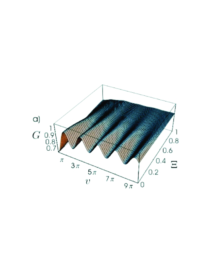
Figure 3: (color online). Conductance plots: in Fig. a) we show the conductance as a function of bias voltage $v$ and temperature $\Xi$ both in units of the non-interacting level spacing $\hbar/t_{\text{{f}}}$ for the strongly correlated case $g=0.23$. The backscattering coefficients are taken at zero temperature as $U^{\rm in}=0.12$, $U^{\rm co}=0.1$. In Fig. b) we compare the conductance at zero temperature for different interaction strengths: $g=0.23$(red), $g=1$(dashed). Fig. c) is devoted to the study of the gate voltage dependence for $g=0.23$: we have chosen $U^{\rm in}=0.12$, $U^{\rm co}=0.1$(red), $U^{\rm in}=0.12$, $U^{\rm co}=-0.1$(dashed), $U^{\rm in}=0.12$, $U^{\rm co}=0$(points).

IV.2 Analytical results

In this subsection we provide an analytical approximation of $I_{B}^{\rm in}$ in the regime where the bias voltage and/or temperature are large compared to the interacting level spacing $\hbar/t_{c}$ where $t_{c}=t_{\text{{f}}}g$ is the charge traversal time along the SWNT. In the non-interacting case $g=1$, we can calculate $I_{B}$ analytically without approximations, including the interference term $I_{B}^{\rm co}$.

Since the correlation time for the backscattering processes is given by $\hbar/eV$ or $\hbar/k_{\rm B}T$ the multiple reflection terms in the retarded and correlation functions [Eqs. (15)-(21)] are not resolved as the traversal time $t_{c}$ is too large. We then take only the $k=0$ contribution in the retarded function [Eq. (IV.1)] and set $\tau$ to zero in the $k\geq 1$ terms in the correlation functions [Eqs. (18) and (20)]. Note that the time $t$ has to be considered as still larger than the cut-off time $\hbar/\epsilon_{0}$.

Figure 4: Comparison of backscattered current $I_{B}$ in units of $G_{0}\hbar/t_{\text{{f}}}e$ at zero temperature (black) with the approximate formula Eq. (24) (dashed) showing the power-law $I_{B}\propto V^{1-\gamma/2}$. In both cases we use $U^{\rm in}=U^{\rm co}=0.1$ and $g=0.23$.

Explicitly, we consider the regime ${\rm max}(eV,k_{\rm B}T)\gg\hbar/t_{c}$ where the incoherent portion $I_{B}^{\rm in}$ of the backscattered current becomes proportional to the integral

$$I_{B}^{\rm in}\propto\sum\limits_{r=\pm}r\int d\tau\frac{\sin(v\tau)}{\sinh[\pi\Xi(r\tau+i\alpha)]^{2\nu}}.$$ (22)

This integral can be expressed in terms of standard functions with the result (in the limit $\alpha\rightarrow 0$)

$$I_{B}^{\rm in}=-\frac{4e}{h}\sum\limits_{ij}\bigl{[}(u_{1}^{ij})^{2}+(u_{2}^{ij})^{2}\bigr{]}k_{\rm B}T\sinh\left(\frac{eV}{2k_{\rm B}T}\right)\\ \times\frac{(2\pi/\epsilon_{0})^{2}}{\Gamma(2-\gamma/2)}\left(\frac{2\pi k_{\rm B}T}{\epsilon_{0}}\right)^{-\gamma/2}\left|\Gamma\left(1-\frac{\gamma}{4}+i\frac{eV}{2\pi k_{\rm B}T}\right)\right|^{2}.$$ (23)

Note that for $g=1$ the temperature dependence drops out and the current is only depending on the bias voltage. This is only true if the transmission is energy independent which is the case for the incoherent contribution $I_{B}^{\rm in}$.

Figure 5: Backscattered current $I_{B}$ in units of $G_{0}\hbar/t_{\text{{f}}}e$ at $v\sim 0.137$ as a function of dimensionless temperature $\Xi$. The continuous line is obtained from numerical integration of Eq. (IV), whereas the dashed line is the approximated incoherent contribution of $I_{B}$ given in Eq. (23). As expected, they agree for temperatures larger than the non-interacting level spacing, i.e $\Xi>1$. For both curves we use $U^{\rm in}=U^{\rm co}=0.1$ and $g=0.23$.

In the high bias regime $eV\gg k_{\rm B}T$ we obtain the power-law scaling on bias voltage

$$I_{B}^{{\rm in}}=-\frac{2e^{2}}{h}V\sum\limits_{ij}\bigl{[}(u_{1}^{ij})^{2}+(u_{2}^{ij})^{2}\bigr{]}\\ \times\frac{(2\pi/\epsilon_{0})^{2}}{\Gamma(2-\gamma/2)}\left(\frac{eV}{\epsilon_{0}}\right)^{-\gamma/2}e^{-eV/\epsilon_{0}}.$$ (24)

The interference contribution proportional to $U^{\rm co}$ describes the FP-interference with two frequencies coming from the total charge mode with velocity $v_{c}$ and three non-interacting modes with velocities $v_{\text{{f}}}$. In general, such integrals are not straightforward to calculate analytically even in the high energy regime unless we set $g=1$.

When $g=1$, we can calculate the backscattered current analytically for all temperatures and bias voltages. The FP-interference contribution $I_{B}^{\rm co}$ then becomes proportional to the integral

$$I_{B}^{{\rm co},g=1}\propto\pi\Xi\int d\tau\frac{e^{i\Omega\tau}-e^{-i\Omega\tau}}{\prod\limits_{r=\pm}\sinh(\tau+r\pi\Xi+i\alpha)},$$ (25)

where $\Omega=v/\pi\Xi$ and $\alpha\rightarrow 0^{+}$. This integral has simple poles (for $\Xi\neq 0$) for $\tau=-r\pi\Xi+in\pi-i\alpha$ where $n=0,\pm 1,\pm 2...$. If $\Omega>0$ we can close the contour in the upper half of the complex plane associated with $e^{i\Omega\tau}$ thereby picking up poles for $n\geq 1$, and in the lower half-plane associated with the term $e^{-i\Omega\tau}$ and picking up poles for $n\leq 0$. All poles except the one for $n=0$ cancel when combining the two contributions. Adding the $g=1$ contribution from Eq. (23) (or Eq. (24) in the limit $\epsilon_{0}\rightarrow\infty$) the result is

$$I_{B}^{g=1}=-\frac{2e^{2}}{h}\left(\frac{2\pi}{\epsilon_{0}}\right)^{2}\biggl{\{}\sum\limits_{ij}\bigl{[}(u_{1}^{ij})^{2}+(u_{2}^{ij})^{2}\bigr{]}V\\ +\sum\limits_{ij}2u_{1}^{ij}u_{2}^{ij}\cos(V_{\rm g}L+2\Delta_{ij})\\ \times\frac{(2\pi k_{\rm B}T/e)}{\sinh(2\pi k_{\rm B}Tt_{\text{{f}}}/\hbar)}\sin\left(\frac{eVt_{\text{{f}}}}{\hbar}\right)\biggr{\}}.$$ (26)

We note that temperature suppresses the FP-interference exponentially if $k_{\rm B}Tt_{\text{{f}}}/\hbar\gg 1$, i.e. if the temperature is much larger than the level spacing.

IV.3 Physical interpretation of dc current results

In Section B we derived the backscattered current and conductance as a function of bias voltage, gate voltage and temperature.

First, we discuss the incoherent contribution of $I_{B}$ which is dominant at large bias voltages. As the energy scale at which the system is probed exceeds the interacting charge mode level spacing $\hbar v_{c}/L$, the TLL-correlations become apparent and our asymptotic formula Eq. (23) applies approximately (see Figs. 4 and 5). At large bias voltages (and small temperatures) we observe the characteristic power-law in Eq. (24). At this energy scale, the $U^{\rm in}$-term (incoherent part) does not resolve the multiple reflections of the charge mode originating from the inhomogeneity of $g$ at the boundaries between SWNT and reservoirs because the traversal time $t_{c}$ becomes larger than the coherence time of electron wave packets given by $\hbar/eV$ or $\hbar/k_{\rm B}T$. In this case, only the $k=0$ term in retarded- and correlation functions contributes significantly. The strength of charge mode ($a=1$) correlations relative to the non-interacting modes $a=2,3,4$ is then given as $1-\gamma$ where $\gamma=(1-g)/(1+g)$. This is apparent from the formula for the retarded function Eq. (IV.1) or in the correlation functions Eqs. (18) and (20). This relative factor $1-\gamma$ is the effective TLL-parameter $g_{{\rm eff}}$ at the boundary connecting a Fermi liquid system (metal reservoir) with an infinite TLL-system Sandler . We therefore conclude that at high voltages (or at high temperatures), a charge $g_{\rm{eff}}e$ gets locally backscattered. Similar, the interference term proportional to $U^{\rm co}$ involves the combination $(1-\gamma)(1+\gamma)=1-\gamma^{2}$ which is the product of two backscattering events at spatially separated places [see Eqs. (16), (19) and (21)]. The $(1+\gamma)$-factor appears because the two backscattered charges can only interfere after the backscattered charge at the second barrier traverses the SWNT and has to be transmitted to the left contact with an additional factor $1+\gamma$ on the way. In general, the power-law behavior of transport can be understood as an energy-dependent renormalization of the bare backscattering amplitudes $u_{m}^{ij}$ due to electron-electron interactions. It is a well known fact that a weak backscatterer grows strong as one approaches low energies, eventually going into the tunneling regime. This is signalled by a divergent power-law at small energies KaneFisher92 . In our calculation we take into account the finite-size effect of the interacting region and therefore will not encounter this divergence as the power-law is only valid above the charge mode level spacing. For sufficiently small bare backscattering amplitudes, the perturbative approach presented in this work is therefore valid at all energy scales. Indeed, at energies below the interacting level spacing, the coherence time of electron wave packets becomes much larger than the traversal time and eventually all multiple reflections contribute. Formally this limit corresponds to $L\rightarrow 0$ or $\tau\rightarrow\infty$ in the time integrals of Eq. (IV) where we can sum up all $k$-terms and getting back the non-interacting functions. Therefore, the backscattered current is linear as $V\rightarrow 0$.

The interference contribution proportional to $U^{\rm co}$ shows not only a reduction of the amplitude when sweeping the bias voltage to higher values but is in principle capable of showing FP-oscillations containing two frequencies, namely $v_{c}/L$ coming from the charge mode $a=1$, and $v_{\text{{f}}}/L$ defining the frequency of the non-interacting modes $a=2,3,4$. However, the visibility of the interacting mode is in general much less pronounced than the non-interacting modes as can be seen in Figs. 3b) and 3c). The reason is two-fold: First, all backscattering processes involve three non-interacting modes and only one interacting mode. Therefore, the contribution of the total charge mode $a=1$ is less pronounced. Second, the interacting mode contribution is further reduced by the smallness of $g_{{\rm eff}}$ which enters as a prefactor in the retarded as well as correlation functions at high energies (i.e. small times $t$). At small energies (i.e. large times $t$), all multiple reflections contribute, and therefore the weight of charge mode oscillations increases, but then the charge mode behaves effectively as a non-interacting mode where the separation of velocities is absent.

A finite temperature, besides triggering the TLL-effect [see Eq. (23)], has an additional impact on suppressing the FP-oscillation amplitude which is also the case for the non-interacting system [see Eq. (26)]. This is caused by the temperature induced smearing of the reservoirs Fermi functions. But note that this suppression becomes exponential at large temperatures whereas the TLL-effect is power-law.

In contrast to the bias voltage or temperature, the gate voltage does not enter as a power-law and leads essentially to a periodic modulation of $U^{\rm co}$, see Eq. (IV). In Ref. 11 it was proposed that changing the gate voltage $V_{\rm g}$ allows to tune the strength of ordinary FP-oscillations ($U^{\rm co}$-term) relative to the incoherent contribution ($U^{\rm in}$-term) which is less sensitive (through a weak gate voltage dependence of $g$). The oscillations contained in the incoherent contribution is an interference effect due to a single impurity: the backscattered charge at the impurity can interfere with the momentum-conserving reflections due to the finite size of the interacting region. Although such a dependence on the gate voltage is expected, we note that the oscillations in the incoherent $U^{\rm in}$-term survive only at small voltages $eV\lesssim\hbar v_{\text{{f}}}/Lg$. This requires that the backscattering must be very small in order for the perturbative treatment to be valid. In contrast, the ordinary oscillations ($U^{\rm co}$-term) due to two barriers are more stable towards higher voltages. We will see that the distinction between the ordinary FP-oscillations and the oscillations due to the finite-size effect of the interacting region is much more apparent in the frequency-dependent shot noise.

V Current noise

The current noise $S(x,\omega)$ can be written in terms of the generating functional Eq. (III.2) as

$$S(x,\omega)=-\frac{8}{\pi}e^{2}\int d\omega^{\prime}\frac{\delta^{2}}{\delta\eta(x,\omega)^{*}\delta\eta(x,\omega^{\prime})}Z^{\eta}\biggr{|}_{\eta=0}.$$ (27)

It is obvious from the general form of the shifted generating functional Eq. (III.2) that we can write the noise as

$$S(x,\omega)=S^{0}(x,\omega)+S_{I}(x,\omega),$$ (28)

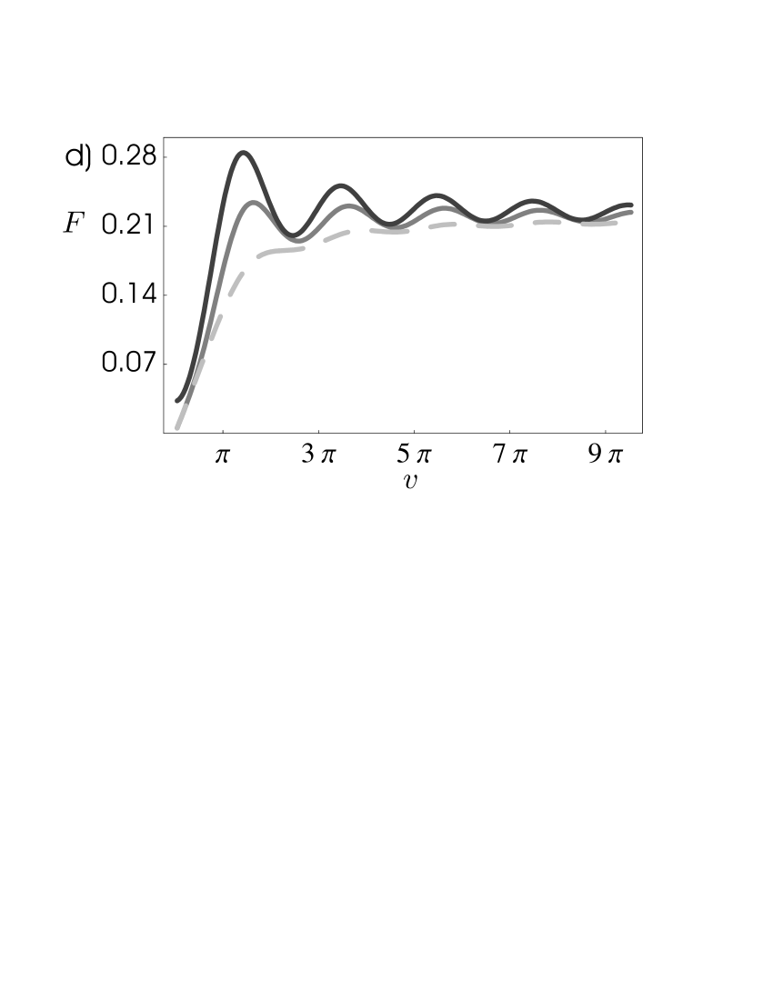
Figure 6: The Fano factor $F$ defined in Eq. (36) for different temperatures and backscattering coefficients. In a) and b) we show the strongly correlated case with $g=0.23$ whereas in c) and d) we present the non-interacting case $g=1$. In a) and c) we use $U^{\rm in}=0.12$ and $U^{\rm co}=0.1$, in b) and d) we use $U^{\rm in}=0.12$ and $U^{\rm co}=-0.1$ at the lowest temperature. The temperatures in units of the non-interacting level spacing $\hbar v_{\text{{f}}}/L$ are: $\Xi=0$(black), $\Xi=0.3$(light gray) and $\Xi=0.7$(dashed).

where $S^{0}(x,\omega)$ is the noise in the absence of backscattering, and the impurity noise $S_{I}(x,\omega)$ is the contribution due to electron backscattering at the SWNT-metal reservoir interfaces. We first give the general result of current noise. This is followed by a discussion of the low-frequency noise and the Fano factor $F=S/eI$ relevant for existing experiments Kim . We then provide an analytical formula for the high-frequency impurity noise for general interaction strength $g$ in terms of the incoherent contribution (only $U^{\rm in}$-contributions) which is the dominant source of noise at high energies. The general numerical evaluation including the FP-interference is presented in Figs. 6-9. In the non-interacting limit $g=1$, we can calculate the noise analytically.

The result for the current noise in the absence of backscattering is

$$S^{0}(x,\omega)=G_{0}\omega\coth\left(\frac{\beta\omega}{2}\right){\rm Re}\,\sigma_{0}(x,x;\omega),$$ (29)

where ${\rm Re}$ means real-part, and we have introduced the dimensionless conductivity conductivity of the clean system without the backscattering $\sigma_{0}(x,y;\omega)=(2i\omega/\pi)R_{1}^{\theta\theta}(x,y;\omega)$. In the following, we will discuss the frequency dependence of the impurity noise $S_{I}$ and refer for simplicity of the discussion to the situation where $\sum_{ij}u_{1}^{ij}u_{2}^{ij}\sin(V_{\rm g}L+2\Delta_{ij})=0$ which can always be reached by tuning the gate voltage. We present the general result in Appendix B. Then, $U^{\rm co}\propto\sum_{ij}u_{1}^{ij}u_{2}^{ij}\cos(V_{\rm g}L+2\Delta_{ij})$ will be maximal for this particular gate voltage. We split the impurity noise in an incoherent part plus a coherent part, $S_{I}(x,\omega)=S_{I}^{\rm in}(x,\omega)+S_{I}^{\rm co}(x,\omega)$. In units of $G_{0}\hbar/t_{\text{{f}}}$ we obtain

$$S_{I}^{\rm in}(x,\omega)= -\frac{et_{\text{{f}}}}{2\hbar G_{0}}\,\sum\limits_{r=\pm}\coth\left(\frac{v+r{\tilde{\omega}}}{2\Xi}\right)\,\sum\limits_{m}\,|\sigma_{0}(x,x_{m};\omega)|^{2}I_{Bm}^{{\rm in}}(v+r{\tilde{\omega}})$$

$$-2\sum\limits_{m}U_{m}^{{\rm in}}\,\coth\left(\frac{{\tilde{\omega}}}{2\Xi}\right){\rm Re}\,\sigma_{0}(x,x_{m};\omega)\,{\rm Im}\left[\sigma_{0}(x,x_{m};\omega)\,\int d\tau\,e^{{\bf C}_{11}(\tau)}\sin[{\bf R}_{11}(\tau)/2]\left(1-e^{i{\tilde{\omega}}\tau}\right)\cos(v\tau)\right],$$

$$S_{I}^{\rm co}(x,\omega)= -\frac{et_{\text{{f}}}}{2\hbar G_{0}}\,{\rm Re}\left\{\sigma_{0}(x,x_{1};\omega)^{*}\sigma_{0}(x,x_{2};\omega)\right\}\sum\limits_{r=\pm}\coth\left(\frac{v+r{\tilde{\omega}}}{2\Xi}\right)\,I_{B}^{{\rm co}}(v+r{\tilde{\omega}})$$

$$-U^{\rm{co}}\,\coth\left(\frac{{\tilde{\omega}}}{2\Xi}\right)\sum\limits_{mm^{\prime}}\,{\rm Re}\,\sigma_{0}(x,x_{m};\omega)$$

$$\times{\rm Im}\left\{\sigma_{0}(x,x_{m^{\prime}};\omega)\int d\tau\,e^{{\bf C}_{12}(\tau)}\sin[{\bf R}_{12}(\tau)/2]\left(\delta_{mm^{\prime}}-(1-\delta_{mm^{\prime}})e^{i{\tilde{\omega}}\tau}\right)\cos(v\tau)\right\}.$$ (30)

In Eq. (V) we need the charge conductivity $\sigma_{0}(x,x_{m};\omega)$ connecting the impurity positions $x_{m}=\pm L/2$ with the point of measurement which we choose to be in the right lead, i.e. $x\geq L/2$ (the result for $x$ in the left lead is easily obtained from Eq. (31) by $x_{1}\leftrightarrow x_{2}$ and $x\rightarrow-x$). In this case we get for the retarded function

$$R_{1}^{\theta\theta}(x,x_{m};\omega)=-\frac{i\pi}{2\omega}(1-\gamma)\frac{e^{i\omega(\frac{x}{L}-\frac{1}{2})t_{\text{{f}}}}}{1-\gamma^{2}e^{i2\omega t_{c}}}\\ \times\left(e^{i\omega(\frac{1}{2}-\frac{x_{m}}{L})t_{c}}+\gamma e^{i\omega(\frac{3}{2}+\frac{x_{m}}{L})t_{c}}\right).$$ (31)

Note that $R_{1}^{\theta\theta}(x,x_{m};\omega)^{*}=R_{1}^{\theta\theta}(x,x_{m};-\omega)$. In Eq. (V) we have introduced the dimensionless frequency ${\tilde{\omega}}=\omega t_{\text{{f}}}$ and the decomposition $I_{B}^{\rm in}=\sum_{m=1,2}I_{Bm}^{\rm in}$.

V.1 Low-frequency noise

In this subsection we investigate the small frequency limit $\omega\rightarrow 0$ of noise.

V.1.1 Noise in the absence of backscattering

We first consider Eq. (29) in the limit of small $\omega$ where $S^{0}(x,\omega)\propto\coth(\beta\omega/2)\omega$. When $k_{\rm B}T\gg\hbar\omega$, we recover the Johnson-Nyquist noise

$$S^{0}(x,\omega)|_{\omega\rightarrow 0}=2k_{\rm B}T\,G_{0},$$ (32)

where we used that for small $\omega$ it holds that $\coth(\beta\omega/2)=2/\beta\omega$. We also restored the units of $\hbar$, i.e. $G_{0}=4e^{2}/h$. In the limit of $k_{\rm B}T\ll\hbar\omega$ we obtain the quantum noise in the absence of the scatterers

$$S^{0}(x,\omega)=\hbar|\omega|G_{0}.$$ (33)

The full frequency dependence of $\sigma_{0}(x,x;\omega)$ contains interference effects of the multiple plasmon reflection inside the nanotube as well as interference terms depending on the measuring point $x$. Instead of elaborating the noise of the clean system further we concentrate on the impurity or shot noise, to be discussed next noteDolcini .

V.1.2 Shot noise

At zero frequency $\omega$, the impurity noise $S_{I}$ adds to the total noise to give

$$S=-e\,\coth\left(\frac{eV}{2k_{\rm B}T}\right)\,I_{B}+2k_{\rm B}TG_{B}+2k_{\rm B}TG,$$ (34)

where $G=G_{0}+G_{B}$ with $G_{B}=dI_{B}/dV$. At zero temperature, the shot noise becomes $S=-e\coth(eV/2k_{\rm B}T)I_{B}$ with $\coth(eV/2k_{\rm B}T)={\rm sgn}(eV)$ at $T=0$. We then finally obtain for the zero temperature noise at zero frequency

$$S=e|I_{B}|.$$ (35)

Note that it is the electron charge $e$ rather than the fractional charge $ge$ in front of $I_{B}$ in contrast to the infinite SWNT with an impurity Smithanoise .

V.1.3 Fano factor

Here we discuss the experimentally relevant Fano factor $F=S/eI$ which is the ratio of the noise to the full shot noise $eI$. The Fano factor is only well defined for the shot noise part of Eq. (34) which is $S-2k_{\rm B}T\,G$. This Fano factor can be written in dimensionless quantities as

$$F=\frac{-\coth\left(\frac{eV}{2k_{\rm B}T}\right)\frac{I_{B}}{I_{0}}+\frac{2k_{\rm B}T}{eV}\frac{G_{B}}{G_{0}}}{\left(1+\frac{I_{B}}{I_{0}}\right)},$$ (36)

where we used that the total current $I=I_{0}+I_{B}$. Note to be consistent with the lowest order expansion in the backscattering, we would have to expand the denominator in Eq. (36) and keep only $I_{0}$. However, this distinction is only essential if the next order would contribute significantly.

  

  

V.2 Analytical results of high-frequency noise

Although an analytical solution of the time integrals in Eq. (V) is not possible we can estimate the general trend for the impurity noise at high energies. We assume that the temperature is close to zero, i.e. $|eV|,|eV\pm\hbar\omega|\gg\hbar/t_{c},k_{\rm B}T$, and obtain for the incoherent part

$$S_{I}^{\rm in}=\sum\limits_{m=1,2}U_{m}^{\rm in}\,|\sigma_{0}(x,x_{m};\omega)|^{2}\,\frac{\pi}{4}\sum\limits_{r=\pm}\coth\left(\frac{|v+r{\tilde{\omega}}|}{2\Xi}\right)\frac{|v+r{\tilde{\omega}}|^{1-\gamma/2}}{\Gamma(2-\gamma/2)}\\ \\ -2\sum\limits_{m}U_{m}^{\rm in}\coth\left(\frac{{\tilde{\omega}}}{2\Xi}\right){\rm Re}\,\sigma_{0}(x,x_{m};\omega)\frac{(\pi/4)}{\Gamma(2-\gamma/2)}\biggl{\{}{\rm Re}\,\sigma_{0}(x,x_{m};\omega)\left({\rm sgn}({\tilde{\omega}}-v)|{\tilde{\omega}}-v|^{1-\gamma/2}+{\rm sgn}({\tilde{\omega}}+v)|{\tilde{\omega}}+v|^{1-\gamma/2}\right)\\ -{\rm Im}\,\sigma_{0}(x,x_{m};\omega)\cot[\pi(2-\gamma)/4](|v+{\tilde{\omega}}|^{1-\gamma/2}+|v-{\tilde{\omega}}|^{1-\gamma/2}-2|v|^{1-\gamma/2})\biggr{\}}.\\$$ (37)

V.2.1 Analytical result for $g=1$

It is worth to examine the non-interacting limit $g=1$ in the above expression where the asymptotic approximation Eq. (37) is exact (note that the temperature dependence of the correlation functions does not contribute when $g=1$, see Eq. (23)). We show now that we essentially get the Landauer-Büttiker result in this case, namely

$$S_{I}^{{\rm in},g=1}=\frac{e^{2}}{2h}\sum\limits_{n}R_{n}\sum\limits_{r=\pm}\coth\left(\frac{eV+r\hbar\omega}{2k_{\rm B}T}\right)(eV+r\hbar\omega)\\ -\frac{2e^{2}}{h}\hbar\omega\coth\left(\frac{\hbar\omega}{2k_{\rm B}T}\right)\left\{\sum\limits_{n}R_{n}^{(1)}\cos^{2}[\omega(L+\Delta x)/v_{\text{{f}}}]\right.\\ \left.+\sum\limits_{n}R_{n}^{(2)}\cos^{2}[\omega\Delta x/v_{\text{{f}}}]\right\},$$ (38)

where $\Delta x=x-L/2\geq 0$. In Eq. (38) we have written the noise in dimensionfull units, and we also introduced reflection coefficients $R_{n}=R_{n}^{(1)}+R_{n}^{(2)}$ for barrier (1) and (2), respectively. They are related to $U^{\rm in}$ by $\frac{e^{2}}{h}\sum_{n}R_{n}=(\pi/2)U^{\rm in}G_{0}$. This choice is motivated by the fact that $I_{B}=-(1/2)I_{0}\pi U^{\rm in}$ in the non-interacting limit (only incoherent contribution considered). To make contact with the Landauer-Büttiker formalism BuBla we write the total current as $I=(e^{2}/h)\sum_{n}T_{n}V$ with $T_{n}=1-R_{n}$ being the transmission coefficient for mode $n$. In our regime of small reflections ($R_{n}\ll 1$) we have $I=I_{0}+I_{B}$ and therefore $I_{B}^{{\rm in},g=1}=-(e^{2}/h)\sum_{n}R_{n}V$. The result Eq. (38) agrees exactly with Eq. (12) in Ref. 40 in the limit of zero temperature and weak backscattering. Eq. (38) coincides with the Landauer-Büttiker formalism only up to the oscillatory terms which depend on the measurement position $x$ and become important if $2\omega(L+\Delta x)/v_{\text{{f}}}\gtrsim 1$. This oscillatory behavior for large frequencies, or equivalently, for measurement points far away from the impurities results from the beat note of finite frequency noise for energies which differ by $\pm\hbar\omega$. The phase difference acquired from the measurement point to the impurities and back will result in the observed interference oscillations.

For $g=1$, we can calculate the interference contribution proportional to $U^{\rm co}$ in closed form. Using $(\pi/2)U^{\rm co}G_{0}=2(e^{2}/h)\sum_{n}\sqrt{R_{n}^{1}R_{n}^{2}}$ and dimensionfull units we obtain

$$S_{I}^{{\rm co},g=1}=-\frac{e^{2}}{h}\frac{2\pi k_{\rm B}T}{\sinh(2\pi k_{\rm B}Tt_{\text{{f}}}/\hbar)}\coth\left(\frac{\hbar\omega}{2k_{\rm B}T}\right)\sum\limits_{n}\sqrt{R_{n}^{1}R_{n}^{2}}\sum\limits_{m\neq m^{\prime}}\sum\limits_{r=\pm}{\rm Re}\,\sigma_{0}(x,x_{m};\omega)\\ \times\left\{{\rm Im}\,\sigma_{0}(x,x_{m^{\prime}};\omega)\cos\left[\frac{(\hbar\omega+reV)t_{\text{{f}}}}{\hbar}\right]+{\rm Re}\,\sigma_{0}(x,x_{m^{\prime}};\omega)\sin\left[\frac{(\hbar\omega+reV)t_{\text{{f}}}}{\hbar}\right]-{\rm Im}\,\sigma_{0}(x,x_{m};\omega)\cos\left(\frac{eVt_{\text{{f}}}}{\hbar}\right)\right\}\\ \\ +\frac{e^{2}}{h}\sum\limits_{n}\sqrt{R_{n}^{1}R_{n}^{2}}\,{\rm Re}\left\{\sigma_{0}(x,x_{1};\omega)^{*}\sigma_{0}(x,x_{2};\omega)\right\}\sum\limits_{r=\pm}\coth\left(\frac{eV+r\hbar\omega}{2k_{\rm B}T}\right)\frac{2\pi k_{\rm B}T}{\sinh(2\pi k_{\rm B}Tt_{\text{{f}}}/\hbar)}\sin\left[\frac{(eV+r\hbar\omega)t_{\text{{f}}}}{\hbar}\right].\\$$ (39)

V.3 Physical interpretation of shot noise results

We first discuss the results for the low-frequency noise. The general result for the low-frequency noise is presented in Eq. (34). This result, valid for finite temperatures, is formally identical to that of an infinite TLL KaneFisher94 except for the important difference that a renormalization of the backscattered charge is absent. This fact is not at all trivial and has first been predicted by Ponomarenko and Nagaosa Nagaosa in the case of a random backscattering potential. Our result shows that this is also true for the SWNT with double barriers. One could argue that the high bias/temperature transport regime is sensitive to interaction (see subsection IV B) and thus a charge $g_{{\rm eff}}e$ in front of the backscattered current appears, rather than the charge $e$. However, this conclusion is wrong. Even if a fractional charge is locally backscattered by the barriers, this charge cannot directly enter the leads, but will further get partially backscattered at the interfaces due to the inhomogeneity of the TLL parameter $g$. Summing over all backscattered partial charges results in the electron charge $e$. The zero-frequency noise is only sensitive to this integral effect as it sums up correlations over all times. Therefore, at low frequencies, the transport process is that of electrons with charge $e$ which are backscattered by a scattering region connecting two Fermi liquid leads. It is interesting that this conclusion is independent of the bias voltage; the regime of low or high bias voltage is only distinguished by the power-laws of transmission. The most pronounced effect of interactions in low-frequency noise or Fano factor is its power-law dependence on bias voltage and temperature.

 

Figure 7: (color online). Excess noise $S_{e}=S(V,\omega)-S(0,\omega)$ in units of $G_{0}\hbar/t_{\text{{f}}}$ at temperature $\Xi=0.3$ for interaction strength $g=0.23$ using numerical integration of Eq. (V). The backscattering coefficients are $U_{1}^{\rm in}=U_{2}^{\rm in}=0.06$ and $U^{\rm co}=0.1$. We have chosen the measurement point to be at one of the barriers. Figure a) shows the excess noise as a function of bias voltage $eV$ and frequency $\hbar\omega$ (both in units of the non-interacting level spacing $\hbar v_{\text{{f}}}/L$). In Plot b) we present the low frequency noise $\omega=0$ as a function of bias voltage. Clear FP-oscillations dominated by the non-intearcting frequency $v_{\text{{f}}}/L$ are seen as well as the power-law scaling with power $1-\gamma/2$. In Plot c) we show the frequency-dependence of excess noise at large bias voltage $v\sim 34$. Dominant charge mode oscillations with frequency $\hbar v_{\text{{f}}}/2Lg$ are observed.

 

Figure 8: (color online). Same parameters as in Fig. 7 but for a non-interacting system with $g=1$. In graph b) approximately the same periodicity of FP-oscillations is found as in the interacting case but the frequency dependence at large bias voltage presented in graph c) is clearly different. Only much smaller ordinary FP-oscillations with frequency $v_{\text{{f}}}/L$ are seen. Superimposed are the additional oscillations depending on the measurement point. For the chosen point of measurement $|x|=L/2$ this oscillation frequency is $v_{\text{{f}}}/2L$.

The finite frequency impurity noise Eq. (V) contains FP-oscillations coming from all collective modes as well as a periodic noise suppression as a function of frequency with the oscillation period determined by the charge mode velocity $v_{c}$. At large bias voltage, this frequency dependence is dominated by the first term on the right-hand-side of Eq. (37). The periodic modulation originates from $|\sigma_{0}(x,x_{m};\omega)|^{2}$ where $x$ is the point of measurement. Interestingly, this term does not depend on $x$ in contrast to the terms $\propto\coth({\tilde{\omega}}/2\Xi)$ in Eq. (37), which, however, are smaller when $eV\gg\hbar\omega$.

Figure 9: The excess noise $S_{e}$ in the same regime as in Figs. 7c) and 8c) but for different measurement points in the leads $|x|>L/2$. In graph a) we present the strongly interacting case $g=0.23$ and in graph b) the non-interacting case $g=1$. We show curves for three different measurement points: $d=0.14$(dark), $d=0.3$(light gray) and $d=0.6$(dashed) where $d$ is the distance from $x$ to the nearest barrier in units of SWNT-length $L$.

Therefore, at high bias voltage and/or low frequencies, the noise clearly shows the oscillations with frequency $v_{c}/2L$. This is indeed observed in Fig. 7. These oscillations are a consequence of the charge fragmentation at the SWNT-metal reservoir interfaces due to the inhomogeneity of $g$. These oscillations have to be distinguished from the oscillations due to standard FP-interferences which contain the frequencies of all modes. At larger frequency $\omega$, the terms $\propto\coth({\tilde{\omega}}/2\Xi)$ in Eq. (37) become important as well. They contain shot noise parts as well as thermal noise parts. This is clear when noting that at zero frequency these terms are the impurity dependent parts of $2k_{\rm B}TG_{B}+2k_{\rm B}TG$ in Eq. (34). With growing frequencies $\omega$, these terms become sensitive to the measurement point $x$. This is clearly seen in the solution for $g=1$ presented in Eqs. (39) and (40). These oscillating factors are a consequence of interference of electron waves which differ in energy by $\hbar\omega$. On the way from the measuring point to the impurities and back these waves will pick up different phases which then results in the oscillation factors, see also Refs. 39 and 23. In principle, these oscillations will influence the noise at every frequency, provided the measurement is taken far away from the scattering region. In reality, however, the metal contacts are not ballistic and therefore these results are only valid for a measurement point $x$ near the barriers (within the inelastic mean-free path of the contacts)Dolcini .

We further comment on Figs 7 and 8 which show the excess noise $S_{e}(V,\omega)=S(V,\omega)-S(0,\omega)$ at low temperature chosen to be $\Xi=0.3$, relevant for experiments. This definition subtracts the noise in the absence of the barriers. In the non-interacting case (Fig. 8) the most striking features are the clear diagonal structure in the 3D-plot 8a) which states that the excess noise is essentially zero when $\hbar\omega>eV$, see Eq. (38). The small oscillations in the excess noise originate from the interference term Eq. (39) and contain the FP-oscillations in both, bias voltage and frequency as well as oscillations as a function of frequency depending on the measurement point [see dependence on $d$ in Fig. 9b)]. The multiple reflections at the boundary between nanotube and contacts are driven by the e-e interactions and therefore these oscillations are absent when $g=1$. Fig. 7 shows the excess noise for a strongly correlated system with $g=0.23$. The low-frequency noise as a function of bias voltage [Fig. 7b)] shows a power-law behavior with exponent $1-\gamma/2$ as well as some minor qualitative differences of the FP-interference oscillations compared to the non-interacting case. But the oscillation period is dominated by the non-interacting frequency. The bias window $\Delta V$ between two maxima is very well approximated by $\Delta V=h/t_{\text{{f}}}e$, i.e. the voltage difference expected for a non-interacting system. The frequency dependent noise at high bias voltage is clearly different from the non-interacting case. Striking are the oscillations of noise with period $\Delta\omega=\pi/t_{c}$ due to the charge flux fragmentation at the SWNT-metal reservoir interfaces. They are much more pronounced than the ordinary FP-oscillations due to two barriers if $eV\gg\hbar v_{\text{{f}}}/L$ since $I_{B}^{\rm in}$ grows monotonically with bias voltage whereas the strength of $I_{B}^{\rm co}$ (showing the FP-oscillations) is bounded roughly by the level spacing $\hbar v_{\text{{f}}}/L$. At low frequencies, these oscillations are clearly resolved. At larger frequencies, oscillations depending on the measurement point are superimposed [see Fig. 9a)]. However, the charge mode oscillation period $\pi/t_{c}$ is still very pronounced. Note, the excess noise is not zero anymore at large frequencies as this is the case in the absence of interaction. This is mainly due to the last term in the asymptotic formula Eq. (37) which depends on the bias voltage. Therefore, the excess noise receives a non-zero contribution from this term. Note that its prefactor $\cot[\pi(2-\gamma)/4]$ vanishes for $g=1$, and, as a consequence, this contribution is absent when $g=1$. The excess noise can even get negative in agreement with Ref. 23. Even if $S_{e}$ is not strictly zero for $\hbar\omega>eV$, there is still a pronounced diagonal structure showing a cusp singularity when $eV=\hbar\omega$.

To observe the high-frequency oscillations we must at least be able to see the first minimum, which translates into $\Delta\omega\sim\pi/2t_{\text{{f}}}g$. To have still ballistic transport we should be well below the mean free path of a carbon nanotube which, at low temperatures can exceed several micrometers. Using $L\sim 10\mu{\rm m}$ this translates into an estimate for the frequency of $\omega/2\pi\lesssim$ 100 GHz which is in the range of existing technology Schoelkopf ; Deblock . A relevant extension of this setup over previously discussed systems Dolcini is achieved through the inclusion of two impurities as well as through the consideration of four modes relevant for a carbon nanotube. In this system, ordinary FP-oscillations as well as oscillations in noise due to the finite length of the interacting region coexist. This allows us to extract the TLL parameter $g$ by comparing the oscillations in bias voltage and as a function of frequency, i.e. building the ratio $\Delta V/\Delta\omega\sim(2\hbar/e)g$ allows to estimate $g$ without referring to power-law fitting and without knowing of any other system parameter like the length $L$ or the precise position of an impurity in the wire Dolcini . We should also mention, that this ratio $\Delta V/\Delta\omega$ contains valuable information about spin-charge separation or in general, information about different velocities of elementary excitations in a carbon nanotube.

VI Conclusions

We have calculated and discussed in detail conductance and finite frequency shot noise in a single-walled carbon nanotube (SWNT) in good contact to electron reservoirs using a non-equilibrium Keldysh functional integral approach. Special focus was put on the interference of backscattering events off two weak impurities naturally formed at the interface between the SWNT and metal contacts. These so called Fabry-Perot (FP) interferences exhibit oscillations in conductance and shot noise as a function of bias voltage and noise frequency which are dominated by the non-interacting traversal time $t_{\text{{f}}}=L/v_{\text{{f}}}$ rather than the interacting velocity $t_{c}=t_{\text{{f}}}g$, with $L$ the SWNT-length and $g$ the Tomonaga-Luttinger liquid parameter, due to two degenerate subbands in the SWNT. However, the finite frequency noise is in addition capable to resolve the splintering (momentum-conserving reflections of fractional charge) of the transported electrons due to the finite length of the interacting SWNT. This dynamics leads to oscillations in the frequency dependent excess noise, which, at large bias voltages, are dominated by a single frequency $(2t_{c})^{-1}$, despite the existence of the ordinary FP-interference oscillations. Therefore, shot noise measurements as a function of bias voltage and frequency seem a decisive tool to distinguish the two mode velocities in the SWNT.

VII Acknowledgments

P. Recher would like to thank L. Balents, M.P.A. Fisher, H. Grabert and N. Nagaosa for helpful comments and discussions. This work is supported by JST/SORST, NTT, University of Tokyo and ARO-MURI grant DAAD19-99-1-0215.

Appendix A Construction of the Keldysh action $S_{0}$

The Keldysh-action $S_{0}$ introduced in Eq. (III.1) is constructed in terms of equilibrium correlation functions between the Keldysh fields. We need the following correlation function (e.g. for the $\theta\phi$-correlation)

$$C^{\theta\phi}_{a}(x,x^{\prime};t) = \langle{\hat{T}}_{K}\theta_{a}(x,t)\phi_{a}(x^{\prime},0)\rangle_{0}$$ (40)

$$= \frac{1}{2}\langle\{{\theta}_{a}(x,t),{\phi}_{a}(x^{\prime},0)\}\rangle_{0},$$

and the retarded functions

$$R^{\theta\phi}_{a}(x,x^{\prime};t) = \langle{\hat{T}}_{K}\theta_{a}(x,t){\tilde{\phi}}_{a}(x^{\prime},0)\rangle_{0}$$ (41)

$$= -i\Theta(t)\,\langle[{\theta}_{a}(x,t),{\phi}_{a}(x^{\prime},0)]\rangle_{0}.$$

The expectation values are taken at equilibrium $V=0$ and in the absence of backscattering $(H_{\rm bs}=0)$. Other combinations like $\langle{\hat{T}}_{K}{\tilde{\theta}}_{a}(x,t){\tilde{\phi}}_{a}(x^{\prime},0)\rangle=\langle{\hat{T}}_{K}{\tilde{\phi}}_{a}(x,t){\tilde{\theta}}_{a}(x^{\prime},0)\rangle=0$. Since the expectation values are determined by the dynamics of $H_{\text{{SWNT}}}$ only, different sectors $a=1...4$ do not mix, i.e. $\langle{\theta}_{a}(x,t){\phi}_{a^{\prime}}(x^{\prime},0)\rangle_{0}=0$ for $a\neq a^{\prime}$. The action $S_{0}$ then can be written as

$$S_{0}=\frac{i}{2}\sum\limits_{a=1}^{4}\int dx\int dx^{\prime}\,\int d\omega\,\left[\theta_{\bf a}^{\rm T}(x,-\omega),\phi_{\bf a}^{\rm T}(x,-\omega)\right]\,G_{\bf a}^{-1}(x,x^{\prime};\omega)\left[\begin{array}[]{c}\theta_{\bf a}(x^{\prime},\omega)\\ \phi_{\bf a}(x^{\prime},\omega)\end{array}\right].$$ (42)

In Eq. (42) the vector ${\bf\theta_{a}}(x,\omega)$ is defined as $\theta_{\bf a}(x,\omega)=[\theta_{a}(x,\omega),{\tilde{\theta}_{a}}(x,\omega)]^{\rm T}$, and similar for $\phi_{\bf a}(x,\omega)$, where, here, T means the matrix transpose. The matrix of the Green’s function operator $G_{\bf a}(x,x^{\prime};\omega)=\langle x|{\bf G_{a}}(\omega)|x^{\prime}\rangle$ is constructed out of the equilibrium correlators and has the representation

$$G_{\bf a}(x,x^{\prime};\omega)=2\pi\,\left(\begin{array}[]{c}C_{a}^{\theta\theta}(x,x^{\prime};\omega)\\ R_{a}^{\theta\theta}(x^{\prime},x;-\omega)\\ C_{a}^{\phi\theta}(x,x^{\prime};\omega)\\ R_{a}^{\theta\phi}(x^{\prime},x;-\omega)\end{array}\begin{array}[]{c}R_{a}^{\theta\theta}(x,x^{\prime};\omega)\\ 0\\ R_{a}^{\phi\theta}(x,x^{\prime};\omega)\\ 0\end{array}\begin{array}[]{c}C_{a}^{\theta\phi}(x,x^{\prime};\omega)\\ R_{a}^{\phi\theta}(x^{\prime},x;-\omega)\\ C_{a}^{\phi\phi}(x,x^{\prime};\omega)\\ R_{a}^{\phi\phi}(x^{\prime},x;-\omega)\end{array}\begin{array}[]{c}R_{a}^{\theta\phi}(x,x^{\prime};\omega)\\ 0\\ R_{a}^{\phi\phi}(x,x^{\prime};\omega)\\ 0\end{array}\right).$$ (43)

It obeys the symmetry $G_{\bf a}(x,x^{\prime};\omega)=G_{\bf a}^{\rm T}(x^{\prime},x;-\omega)$ which follows from the property $C_{a}^{\theta\phi}(x,x^{\prime};\omega)=C_{a}^{\phi\theta}(x^{\prime},x;-\omega)$, (and similar for $\theta\theta$ and $\phi\phi$-correlations) which is evident from the defining Eq. (40).

Appendix B Details of noise calculation

In this appendix, we provide some details of the noise calculations. Starting from Eq. (27) we perform the functional derivatives and obtain to leading order in $H_{\rm bs}$

$$S(x,\omega)=\frac{4}{\pi^{2}}e^{2}\omega^{2}C_{1}^{\theta\theta}(x,x;\omega)-\frac{8}{\pi^{2}}e^{2}\,\sum\limits_{\bf n}\sum\limits_{mm^{\prime}}\,\int dt\,u_{m}^{\bf n}u_{m^{\prime}}^{\bf n}\cos(eVt+\varphi_{mm^{\prime}}^{{\bf n}})\\ \times\sum\limits_{rr^{\prime}=\pm}rr^{\prime}\,f_{m}^{r}(x,\omega)\left[f_{m}^{r}(x,-\omega)-e^{-i\omega t}f_{m^{\prime}}^{r^{\prime}}(x,-\omega)\right]\,\left\langle e^{i[A_{m{\bf n}}^{r}(t)-A_{m^{\prime}{\bf n}}^{r^{\prime}}(0)]}\right\rangle_{0},$$ (44)

where $f_{m}^{\pm}(x,\omega)=\omega\,[C_{1}^{\theta\theta}(x_{m},x;\omega)\pm\frac{i}{2}R_{1}^{\theta\theta}(x,x_{m};-\omega)]$ and the phase operators are $A_{mijs}^{\pm}(t)={\theta}_{1m}^{\pm}+s\theta_{2m}^{\pm}+(-1)^{i+1}\delta_{ij}(\theta_{3m}^{\pm}+s\theta_{4m}^{\pm})+(-1)^{i+1}(1-\delta_{ij})(\phi_{3m}^{\pm}+s\phi_{4m}^{\pm})$ and $\varphi_{mm^{\prime}}^{{\bf n}}=(V_{\rm g}L+2\Delta_{{\bf n}})(m-m^{\prime})$. Further, we introduced the index ${\bf n}=ijs$ and the abbreviation $\langle...\rangle_{0}=\prod_{a}\int{\cal D}[\theta_{a}^{\pm}\phi_{a}^{\pm}]...\exp[iS_{0}]$. We assume now that the current is measured in the right lead (the result for $x$ in the left lead is easily obtained by $x_{1}\leftrightarrow x_{2}$ and $x\rightarrow-x$), i.e. $x\geq L/2$. The general expression for the retarded function in that case reads (see Appendix C)

$$R_{1}^{\theta\theta}(x,x_{m};\omega)=-\frac{i\pi}{2{\omega}}(1-\gamma)\frac{e^{i\omega(\frac{x}{L}-\frac{1}{2})t_{\text{{f}}}}}{1-\gamma^{2}e^{i2\omega t_{c}}}\\ \times\left(e^{i\omega(\frac{1}{2}-\frac{x_{m}}{L})t_{c}}+\gamma e^{i\omega(\frac{3}{2}+\frac{x_{m}}{L})t_{c}}\right).$$ (45)

Note that $R_{1}^{\theta\theta}(x,x_{m};\omega)^{*}=R_{1}^{\theta\theta}(x,x_{m};-\omega)$. The correlation functions are related to the retarded functions via the fluctuation dissipation theorem $C_{1}^{\theta\theta}(x,x_{m};\omega)=C_{1}^{\theta\theta}(x_{m},x;\omega)=-\coth(\beta\omega/2)\,{\rm Im}R_{1}^{\theta\theta}(x,x_{m};\omega)$, where ${\rm Im}$ denotes imaginary part. The expectation value in Eq. (44) is of the general form ($\varepsilon,\varepsilon^{\prime}=+,-$)

$$\left\langle e^{i\varepsilon A_{m{\bf n}}^{r}(t^{\prime})}e^{-i\varepsilon^{\prime}A_{m^{\prime}{\bf n}}^{r^{\prime}}(t^{\prime\prime})}\right\rangle_{0}=e^{-\frac{1}{2}\langle[A_{m{\bf n}}^{r}(t^{\prime})-\varepsilon\varepsilon^{\prime}A_{m^{\prime}{\bf n}}^{r^{\prime}}(t^{\prime\prime})]^{2}\rangle_{0}},$$ (46)

where we used that the action $S_{0}$ is quadratic in the bosonic fields $\theta_{a}^{\pm}$ and $\phi_{a}^{\pm}$ which allows to perform the average in the exponent. The correlator in the exponent of the right-hand-side (RHS) of Eq. (46) always (i.e. for general ${\bf n}$) contains a sum of three non-interacting modes $a=2,3,4$ due to spin and subband degeneracy plus one interacting mode of the total charge $a=1$:

$$\left\langle\left(A_{m{\bf n}}^{r}(t^{\prime})\pm A_{m^{\prime}{\bf n}}^{r^{\prime}}(t^{\prime\prime})\right)^{2}\right\rangle_{0}=\\ \left\langle\sum\limits_{a=1}^{2}\left(\theta_{am}^{r}(t^{\prime})\pm\theta_{am^{\prime}}^{r^{\prime}}(t^{\prime\prime})\right)^{2}+\delta_{ij}\sum\limits_{a=3}^{4}\left(\theta_{am}^{r}(t^{\prime})\pm\theta_{am^{\prime}}^{r^{\prime}}(t^{\prime\prime})\right)^{2}\right.\\ \left.+(1-\delta_{ij})\sum\limits_{a=3}^{4}\left(\phi_{am}^{r}(t^{\prime})\pm\phi_{am^{\prime}}^{r^{\prime}}(t^{\prime\prime})\right)^{2}\right\rangle_{0}.$$ (47)

Note that the correlator above depends on the different processes of interband $i\neq j$ or intraband $i=j$ scatterings which, however, leads to the same correlation functions and only the scattering phases hidden in $U^{\rm co}$ distinguish the different processes. Also note that the correlation functions do not depend on the spin direction $s$. We find [e.g or the $\theta$-fields (similar for $\phi$-fields)]

$$\left\langle\left(\theta_{am}^{r}(t)\pm\theta_{am^{\prime}}^{r^{\prime}}(0)\right)^{2}\right\rangle_{0}=\\ \pm 2C_{a|mm^{\prime}}^{\theta\theta}(t)+2C_{a|mm}^{\theta\theta}(0)\\ \pm\frac{i}{2}(r^{\prime}-r)\left[R_{a|mm^{\prime}}^{\theta\theta}(t)-R_{a|m^{\prime}m}^{\theta\theta}(-t)\right]\\ \pm\frac{i}{2}(r+r^{\prime})\left[R_{a|mm^{\prime}}^{\theta\theta}(t)+R_{a|m^{\prime}m}^{\theta\theta}(-t)\right],$$ (48)

where we have simplified the notation for clarity of the presentation: $C_{a|mm^{\prime}}^{\theta\theta}(t)\equiv C_{a}^{\theta\theta}(x_{m},x_{m^{\prime}};t)$ and $R_{a|mm^{\prime}}^{\theta\theta}(t)\equiv R_{a}^{\theta\theta}(x_{m},x_{m^{\prime}};t)$. We note that only the – sign in Eq. (48) contributes as $\exp[-(1/2)\langle(\theta_{am}^{r}(t)+\theta_{am^{\prime}}^{r^{\prime}}(0))^{2}\rangle]\propto\exp(-\infty)$ due to the first line of the RHS in Eq. (48). This is a direct consequence of particle conservation particleconservation since the + sign option comes from terms like $\langle\psi_{L}^{\dagger}\psi_{R}\psi_{L}^{\dagger}\psi_{R}\rangle_{0}$. The general form of the noise described by Eq. (44) can be split into a sum of a clean limit with no backscattering corrections $S^{0}(x,\omega)$ and the backscattered correction $S_{I}(x,\omega)$ which we refer to as the impurity noise. The clean limit can be written in a more standard form Dolcini using the relation between retarded and correlation function

$$S^{0}(x,\omega)=G_{0}\omega\coth\left(\frac{\beta\omega}{2}\right){\rm Re}\,\sigma_{0}(x,x;\omega),$$ (49)

where ${\rm Re}$ means real-part and we have introduced the dimensionless conductivity conductivity of the clean system without the backscattering $\sigma_{0}(x,y;\omega)=(2i\omega/\pi)R_{1}^{\theta\theta}(x,y;\omega)$. The impurity contribution to the noise $S_{I}(x,\omega)$ can be calculated using Eq. (44) and Eqs. (47) and (48). We obtain after some calculation the general result valid for all temperatures, frequencies, gate voltages and to leading order in the backscattering Hamiltonian $H_{\rm bs}$ (in units of $G_{0}\hbar/t_{\text{{f}}}$)

$$S_{I}(x,\omega)=-2\coth\left(\frac{{\tilde{\omega}}}{2\Xi}\right)\sum\limits_{m}U_{m}^{\rm in}\,{\rm Re}\,\sigma_{0}(x,x_{m};\omega)\\ \times{\rm Im}\left[\sigma_{0}(x,x_{m};\omega)\,\int d\tau\,e^{{\bf C}_{11}(\tau)}\sin[{\bf R}_{11}(\tau)/2]\left(1-e^{i{\tilde{\omega}}\tau}\right)\cos(v\tau)\right]\\ -\frac{1}{2}\sum\limits_{m}U_{m}^{\rm in}\,|\sigma_{0}(x,x_{m};\omega)|^{2}\,\sum\limits_{r=\pm}\coth\left(\frac{v+r{\tilde{\omega}}}{2\Xi}\right)\,\int d\tau\,e^{{\bf C}_{11}(\tau)}\sin[{\bf R}_{11}(\tau)/2]\sin[(v+r{\tilde{\omega}})\tau]\\$$ (50)

$$-\coth\left(\frac{{\tilde{\omega}}}{2\Xi}\right)\sum\limits_{mm^{\prime}}\,{\rm Re}\,\sigma_{0}(x,x_{m};\omega)\\ \times{\rm Im}\left\{\sigma_{0}(x,x_{m^{\prime}};\omega)\,\int d\tau\,e^{{\bf C}_{12}(\tau)}\,\sin[{\bf R}_{12}(\tau)/2]\left(\delta_{mm^{\prime}}-(1-\delta_{mm^{\prime}})e^{i{\tilde{\omega}}\tau}\right)\bigl{[}U^{\rm co}\,\cos(v\tau)-V^{\rm co}(1-2\delta_{1m^{\prime}})\sin(v\tau)\bigr{]}\right\}\\ +\frac{1}{2}\,{\rm Re}\left\{\sigma_{0}(x,x_{1};\omega)^{*}\sigma_{0}(x,x_{2};\omega)\,\int d\tau\,e^{{\bf C}_{12}(\tau)}\cos[{\bf R}_{12}(|\tau|)/2]\,e^{i{\tilde{\omega}}\tau}\bigl{[}U^{\rm co}\cos(v\tau)-V^{\rm co}\sin(v\tau)\bigl{]}\right\}.$$ (51)

In Eq. (50) we have used ${\bf R}_{mm^{\prime}}(\tau)=R_{mm^{\prime}}^{\rm I}(\tau)+3R_{mm^{\prime}}^{\rm F}(\tau)$ and a similar definition holds for ${\bf C}_{mm^{\prime}}(\tau)$. The superscripts ${\rm I}$ and ${\rm F}$ denote interacting and free, respectively. The interacting functions are $\theta_{1}\theta_{1}$-correlations whereas the free functions come from correlations of the non-interacting modes $a=2,3,4$. In the main text we give the slightly more compact result for the case where the coherent (FP)-contribution is maximum, i.e. when $|U^{\rm co}|$ is maximum as a function of gate voltage. In Eq. (50) we have introduced $V^{\rm co}$ which is just $U^{\rm co}$ with $\cos(V_{\rm g}L+2\Delta_{ij})$ replaced by $\sin(V_{\rm g}L+2\Delta_{ij})$. We see that at finite frequency $\omega$, the impurity noise becomes sensitive to the real and imaginary parts of the conductance $\sigma_{0}(x,x_{m};\omega)$ which contains the multiple reflections of the charge mode $a=1$ at the inhomogeneity of $g$ where the SWNT is connected to the non-interacting reservoirs. The complete noise as a function of frequency and bias voltage is therefore a complicated superposition of ordinary FP-oscillations described by the time integrals which are influenced by both, voltage and frequency and exhibit by all four modes whereas the additional frequency response due to $\sigma_{0}(x,x_{m};\omega)$ is only sensitive to the total charge mode $a=1$. For clarity, we give here the explicit form of real and imaginary-parts of the retarded Green’s function connecting the two barriers with the measurement point $x$ (assumed to be in the right lead). For the retarded function with $x_{m}=-L/2$ we obtain from Eq. (45)

$$R_{1}^{\theta\theta}(x,x_{1};\omega)=\frac{\pi}{2\omega}\frac{1-\gamma^{2}}{1-2\gamma^{2}\cos(2\omega t_{c})+\gamma^{4}}\left\{\sin\left[\omega t_{\text{{f}}}(g+d)\right]+\gamma^{2}\sin\left[\omega t_{\text{{f}}}(g-d)\right]\right\}\\ -i\,\frac{\pi}{2\omega}\frac{1-\gamma^{2}}{1-2\gamma^{2}\cos(2\omega t_{c})+\gamma^{4}}\left\{\cos\left[\omega t_{\text{{f}}}(g+d)\right]-\gamma^{2}\cos\left[\omega t_{\text{{f}}}(g-d)\right]\right\}.$$ (52)

For the retarded function with $x_{m}=+L/2$ we obtain

$$R_{1}^{\theta\theta}(x,x_{2};\omega)=\frac{\pi}{2\omega}\frac{1-\gamma}{1-2\gamma^{2}\cos(2\omega t_{c})+\gamma^{4}}\left\{\sin\left(\omega t_{\text{{f}}}d\right)\,[1+\gamma(1-\gamma)\cos(2\omega t_{c})-\gamma^{3}]\right.\left.+\gamma(1+\gamma)\cos\left(\omega t_{\text{{f}}}d\right)\,\sin(2\omega t_{c})\right\}\\ \\ -i\,\frac{\pi}{2\omega}\frac{1-\gamma}{1-2\gamma^{2}\cos(2\omega t_{c})+\gamma^{4}}\left\{\cos\left(\omega t_{\text{{f}}}d\right)[1+\gamma(1-\gamma)\cos(2\omega t_{c})-\gamma^{3}]\right.-\left.\gamma(1+\gamma)\sin\left(\omega t_{\text{{f}}}d\right)\,\sin(2\omega t_{c})\right\}.$$ (53)

In Eqs. (52) and (53) we have introduced the distance from the measurement point $x$ to the nearest metal contact-SWNT interface (here $x_{2}=L/2$) in units of the length $L$ of the nanotube, i.e. $d=(x-x_{2})/L$.

For completeness, we also show a more direct way to obtain the low-frequency noise Eq. (34) starting from Eq. (44) using a low-frequency expansion in $\omega$. For this we consider the term $\sum_{rr^{\prime}}rr^{\prime}f_{m}^{r}(x,\omega)[f_{m}^{r}(x,-\omega)-\exp(-i\omega t)f_{m^{\prime}}^{r^{\prime}}(x,-\omega)]$ in the limit $\omega\rightarrow 0$. To proceed in the evaluation we first make a straightforward expansion of the above expression. We write the function $f_{m}^{r}(x,\omega)$ in terms of real- and imaginary parts of the retarded function $R_{1}^{\theta\theta}(x,x_{m};\omega)$ as

$$f_{m}^{r}(x,\omega)=\omega\left[\left(\frac{r}{2}-\coth\left(\frac{\beta\omega}{2}\right)\right)\,{\rm Im}\,R_{1}^{\theta\theta}(x,x_{m};\omega)\right.\\ \left.\qquad+\frac{i}{2}r{\rm Re}\,R_{1}^{\theta\theta}(x,x_{m};\omega)\right].$$ (54)

We now use the low-frequency behavior of the real- and imaginary part of the retarded functions in Eq. (54) which we express as

$${\rm Re}\,R_{1}^{\theta\theta}(x,x_{m};\omega)=R_{1}^{\theta 0}(x,x_{m})+{\cal O}(\omega^{2})$$ (55)

and

$${\rm Im}\,R_{1}^{\theta\theta}(x,x_{m};\omega)=-\frac{\pi}{2\omega}+R_{1}^{\theta 1}(x,x_{m})\omega,$$ (56)

where $R_{1}^{\theta 0}(x,x_{m})$ and $i\,R_{1}^{\theta 1}(x,x_{m})$ are the zeroth-order and 1st-order expansion coefficient of $R_{1}^{\theta\theta}(x,x_{m};\omega)$, respectively. They depend on $x$, $x_{m}$ and $g$ but we find that these terms will not contribute to the zero-frequency limit of noise. As a consequence, the low-frequency noise is independent on the position of measurement. In this limit, we obtain for the frequency dependent part of Eq. (44)

$$rr^{\prime}\,f_{m}^{r}(x,\omega)\left[f_{m}^{r}(x,-\omega)-\exp(-i\omega t)f_{m^{\prime}}^{r^{\prime}}(x,-\omega)\right]$$

$$= (r-r^{\prime})\left(\frac{\pi}{2}\right)^{2}k_{\rm B}T\left(\frac{1}{\omega}-it\right)-it\,rr^{\prime}\frac{(\pi k_{\rm B}T)^{2}}{\omega}$$

$$- \frac{rr^{\prime}}{2}(\pi k_{\rm B}T)^{2}t^{2}-(1-rr^{\prime})\left(\frac{\pi}{4}\right)^{2}$$

$$+ 2\pi\left(k_{\rm B}T\right)^{2}rr^{\prime}\left(R_{1}^{\theta 1}(x,x_{m})-R_{1}^{\theta 1}(x,x_{m^{\prime}})\right)$$

$$- i\frac{\pi}{2}k_{\rm B}T\left(r^{\prime}R_{1}^{\theta 0}(x,x_{m})-rR_{1}^{\theta 0}(x,x_{m^{\prime}})\right)$$

$$+ {\cal O}(\omega).$$ (57)

By performing the sum over $rr^{\prime}$ as well as the sum over $mm^{\prime}$ we find that the time integral in Eq. (44) yields zero for the terms associated with the $1/\omega$ contributions in Eq. (B). Therefore, the limit $\omega\rightarrow 0$ is well defined. Note also that the voltage term $\cos(eVt+\varphi_{mm^{\prime}}^{{\bf n}})=\cos(eVt)\cos(\varphi_{mm^{\prime}}^{{\bf n}})-\sin(eVt)\sin(\varphi_{mm^{\prime}}^{{\bf n}})$ where, due to the symmetry in the sum over $mm^{\prime}$, only the cosine-terms contribute. Using Eq. (B) in Eq. (44) for the noise we obtain the low-frequency noise presented in Eq. (34).

Appendix C Derivation of retarded and correlation functions

In this appendix, we outline the derivation of the retarded Green’s functions which are calculated in the equilibrium system and without the backscattering ($H_{\rm bs}$=0). We choose to calculate the temperature Green’s function first and then rotate back to real time (Wick rotation) which gives us the retarded function.

We start with deriving the action from the Hamiltonian $H_{\text{{swnt}}}$

$${\cal L}(\Pi_{a},\theta_{a})=\int dx\sum\limits_{a}\,\left[\Pi_{a}(x){\dot{\theta}}_{a}(x)-H_{\text{{swnt}}}(\Pi_{a},\theta_{a})\right].$$ (58)

The action is defined as the time integrated Lagrangian $S=\int dt{\cal L}(t)$. We then change to imaginary time $\tau=it$ and introduce the Euclidean action by the standard identification $-S_{E}=iS(it\rightarrow\tau)$. This immediately gives

$$S_{E}= \frac{1}{2}\sum\limits_{a}\int_{0}^{\beta}d\tau\int dx$$

$$\times \left[i\frac{2}{\pi}\partial_{x}\phi_{a}\partial_{\tau}\theta_{a}+\frac{v_{\text{{f}}}}{\pi}[(\partial_{x}\phi_{a})^{2}+\frac{1}{g_{a}^{2}}(\partial_{x}\theta_{a})^{2}]\right].$$

To calculate time-ordered correlation functions $\langle{\hat{T}}{\hat{A}}({\bf x}){\hat{B}}({\bf x}^{\prime})\rangle$ where ${\hat{A}}$ and ${\hat{B}}$ are any function of operators ${\theta}_{a}$ and ${\phi}_{a}$ we can use the functional integral approach

$$\langle{\hat{T}}{\hat{A}}({\bf x}){\hat{B}}({\bf x}^{\prime})\rangle=\frac{1}{Z}\prod_{a}\int{\cal D}[\phi_{a}\theta_{a}]\,A({\bf x})B({\bf x}^{\prime})e^{-S_{E}(\theta_{a},\phi_{a})},$$ (60)

where ${\bf x}=(x,\tau)$ and $Z=\prod_{a}\int{\cal D}[\phi_{a}\theta_{a}]\,e^{-S_{E}(\theta_{a},\phi_{a})}$ is the partition function. Here, since the bosonic fields are hermitesch, the functional integral is over real-valued fields. If the operators ${\hat{A}}$ and ${\hat{B}}$ are only functions of one of the field-type, i.e. only a function of either ${\theta_{a}}$ or ${\phi_{a}}$, we can integrate out the other variable to get an effective action which only depends on one of the variables. To do this we use the result for Gaussian integration over multidimensional real variables $x_{i},\,i=1,...,N$

$$\prod_{i}\int dx_{i}\,e^{-\frac{1}{2}\sum\limits_{ij}\,x_{i}A_{ij}x_{j}+\sum\limits_{i}\lambda_{i}x_{i}}=\frac{(2\pi)^{N/2}}{\sqrt{{\rm detA}}}\,e^{\frac{1}{2}\sum\limits_{ij}\,\lambda_{i}A_{ij}^{-1}\lambda_{j}},$$ (61)

where det means the determinant of the real symmetric and positive definite matrix $A_{ij}$. We first derive the action for the $\theta_{a}-$ fields. Using partial integration in the action $S_{E}$ we can bring the functional integral Eq. (60) to the form of Eq. (61) with identifying $\lambda_{i}\equiv(i/\pi)\partial_{x}\partial_{\tau}\theta_{a}$ and the matrix elements $A_{ij}\equiv-(v_{\text{{f}}}/\pi)\partial_{x}^{2}\delta(x-x^{\prime})\delta(\tau-\tau^{\prime})$. Note that the determinant will cancel with the similar integration procedures in the partition function. Therefore, for calculating correlation functions the explicit calculation of the determinant in Eq. (61) is not needed. We then obtain the effective action for the $\theta_{a}-$ fields

$$S^{\theta}_{E}=\frac{1}{2\pi}\sum_{a}\int_{0}^{\beta}d\tau\int dx\left[\frac{v_{a}}{g_{a}}(\partial_{x}\theta_{a})^{2}+\frac{1}{g_{a}v_{a}}(\partial_{\tau}\theta_{a})^{2}\right].$$ (62)

Similarly, for the effective action of $\phi_{a}-$fields we obtain

$$S^{\phi}_{E}=\frac{1}{2\pi}\sum_{a}\int_{0}^{\beta}d\tau\int dx\left[v_{a}g_{a}(\partial_{x}\phi_{a})^{2}+\frac{g_{a}}{v_{a}}(\partial_{\tau}\phi_{a})^{2}\right].$$ (63)

We can now use the effective actions to calculate the correlation functions $\langle{\hat{T}}\theta_{a}({\bf x})\theta_{a}({\bf x}^{\prime})\rangle$ and $\langle{\hat{T}}\phi_{a}({\bf x})\phi_{a}({\bf x}^{\prime})\rangle$, respectively.
The relation between functional integrals and time-ordered correlation functions Eq. (60) (e.g. for $\theta_{a}$-fields)

$$\langle{\hat{T}}{\theta}_{a}({\bf x}){\theta}_{a}({\bf x}^{\prime})\rangle=\frac{1}{Z^{\theta_{a}}}\int{\cal D}\theta_{a}\,\theta_{a}({\bf x})\theta_{a}({\bf x}^{\prime})e^{-S_{E}(\theta_{a})}$$ (64)

can also be written as

$$\langle{\hat{T}}{\theta}_{a}({\bf x}){\theta}_{a}({\bf x}^{\prime})\rangle=\left.\frac{\delta^{2}}{\delta\lambda(\bf x)\delta\lambda(\bf x^{\prime})}\,Z^{\lambda}_{\theta_{a}}\right|_{\lambda=0},$$ (65)

where

$$Z_{\theta_{a}}^{\lambda}=\frac{1}{Z^{\theta_{a}}}\int{\cal D}\theta_{a}\,e^{-S_{E}^{\theta_{a}}+\int d{\bf x}\,\lambda({\bf x})\,\theta_{a}({\bf x})}$$ (66)

is the generating functional for the $\theta_{a}$-field. Writing the action $S_{E}^{\theta_{a}}$ as a bilinear form $S_{E}^{\theta_{a}}=(1/2)\int d{\bf x}\int d{\bf x^{\prime}}\theta_{a}({\bf x})[{\hat{G}}_{a}^{\theta\theta}]^{-1}({\bf x},{\bf x^{\prime}})\theta_{a}({\bf x}^{\prime})$ and using the result for Gaussian integration Eq. (61) we conclude that $\langle{\hat{T}}{\theta}_{a}({\bf x}){\theta}_{a}({\bf x}^{\prime})\rangle={\hat{G}}_{a}^{\theta\theta}({\bf x},{\bf x^{\prime}})$ accompanied with the operator statement

$$\left[{\hat{G}}_{a}^{\theta\theta}\right]^{-1}{\hat{G}}_{a}^{\theta\theta}={\hat{1}}.$$ (67)

Using that the inverse Green’s function operator ${\hat{G}}^{-1}$ is local in (imaginary)time and space, i.e. $\langle{\bf x}|{\hat{G}}^{-1}|{\bf x}^{\prime}\rangle={\hat{D}}({\bf x})\delta({\bf x}-{\bf x}^{\prime})$, leads us to the differential equation for the Green’s function in imaginary time

$${\hat{D}}(x,\tau)G(x,\tau;x^{\prime},\tau^{\prime})=\delta(x-x^{\prime})\delta(\tau-\tau^{\prime}).$$ (68)

Eq. (68) clearly shows that the Green’s function is symmetric in ${\bf x}$ and ${\bf x}^{\prime}$. Explicitly, we obtain the differential-operators ${\hat{D}}^{\theta\theta}_{a}({\bf x})=-\frac{1}{\pi}[\frac{1}{v_{a}g_{a}}\partial_{\tau}^{2}+\partial_{x}\frac{v_{a}}{g_{a}}\partial_{x}]$ and ${\hat{D}}^{\phi\phi}_{a}({\bf x})=-\frac{1}{\pi}[\frac{g_{a}}{v_{a}}\partial_{\tau}^{2}+\partial_{x}v_{a}g_{a}\partial_{x}]$. Due to the inhomogeneity of the charge mode $a=1$, its Green’s functions are not translational invariant. The time translation invariance although still holds, i.e. $G(x,\tau;x^{\prime},\tau^{\prime})=G(x,x^{\prime};\tau-\tau^{\prime})$ and we can transform to frequency space using the Fourier expansion for boson Matsubara Green’s functions

$$G(x,x^{\prime};\tau)=\frac{1}{\beta}\sum\limits_{\omega_{n}}e^{-i\omega_{n}\tau}G(x,x^{\prime};\omega_{n}),$$ (69)

where the sum is over the Matsubara frequencies $\omega_{n}=2\pi n/\beta$ with $n=0,\pm 1,\pm 2$. We then obtain a differential equation for the Fourier component of the Matsubara Green’s function

$$\left(\frac{1}{g_{a}v_{a}}\omega_{n}^{2}-\partial_{x}\frac{v_{a}}{g_{a}}\partial_{x}\right)G_{a}^{\theta\theta}(x,x^{\prime};\omega_{n})=\pi\delta(x-x^{\prime}),$$ (70)

and

$$\left(\frac{g_{a}}{v_{a}}\omega_{n}^{2}-\partial_{x}v_{a}g_{a}\partial_{x}\right)G_{a}^{\phi\phi}(x,x^{\prime};\omega_{n})=\pi\delta(x-x^{\prime}).$$ (71)

The solution to these partial differential equations for the case $|x^{\prime}|<L/2$ can be found by the ansatz MaslovStone (for the $\theta\theta$-contribution)

$$G_{a}^{\theta\theta}(x,x^{\prime};\omega_{n})=$$ (76)

$$\left\{\begin{array}[]{lll}Ae^{|\omega_{n}|x/v_{\text{{f}}}};&x\leq-L/2\\ Be^{|\omega_{n}|x/v_{a}}+Ce^{-|\omega_{n}|x/v_{a}};&-L/2<x\leq x^{\prime}<L/2\\ De^{|\omega_{n}|x/v_{a}}+Ee^{-|\omega_{n}|x/v_{a}};&-L/2<x^{\prime}<x\leq L/2\\ Fe^{-|\omega_{n}|x/v_{\text{{f}}}};&x>L/2\\ \end{array}\right.$$

These solutions satisfy the boundary condition $G_{a}^{\theta\theta}(\pm\infty,x^{\prime};\omega_{n})=0$. The coefficients $A-F$ are functions of $x^{\prime}$ and $\omega_{n}$ and can be found from the following boundary conditions

$$\begin{array}[]{lll}{\bullet}\,G_{a}^{\theta\theta}(x,x^{\prime};\omega_{n})\,\,{\rm is\,\,continuous\,\,everywhere}.\\ {\bullet}\,\frac{v_{a}(x)}{g_{a}(x)}\partial_{x}G_{a}^{\theta\theta}(x,x^{\prime};\omega_{n})\,{\rm\,\,is\,\,continuous\,\,at}\,\,x=L/2,-L/2.\\ {\bullet}\,-\frac{v_{a}(x)}{g_{a}(x)}\partial_{x}G_{a}^{\theta\theta}(x,x^{\prime};\omega_{n})\,\,{\rm has\,\,a\,\,step\,\,of\,\,height}\,\,\pi\,\,{\rm at}\,\,x=x^{\prime}.\end{array}$$

These three conditions lead to the following set of equations which can be used to determine all constants $A-F$:

$$\begin{array}[]{l}A=Be^{|\omega_{n}|L(1-g_{a})/2v_{\text{{f}}}}+Ce^{|\omega_{n}|L(1+g_{a})/2v_{\text{{f}}}}\\ F=De^{|\omega_{n}|L(1+g_{a})/2v_{\text{{f}}}}+Ee^{|\omega_{n}|L(1-g_{a})/2v_{\text{{f}}}}\\ C+Be^{2|\omega_{n}|x^{\prime}/v_{a}}=E+De^{2|\omega_{n}|x^{\prime}/v_{a}}\\ g_{a}A=Be^{|\omega_{n}|L(1-g_{a})/2v_{\text{{f}}}}-Ce^{|\omega_{n}|L(1+g_{a})/2v_{\text{{f}}}}\\ g_{a}F=Ee^{|\omega_{n}|L(1-g_{a})/2v_{\text{{f}}}}-De^{|\omega_{n}|L(1+g_{a})/2v_{\text{{f}}}}\\ B-D+(E-C)e^{-2|\omega_{n}|x^{\prime}/v_{a}}=\frac{g_{a}\pi}{|\omega_{n}|}e^{-|\omega_{n}|x^{\prime}/v_{a}}\\ \end{array}$$

The retarded Green’s function $R^{\theta\theta}_{a}(x,t;x^{\prime},t^{\prime})=-i\Theta(t-t^{\prime})\langle[\theta_{a}(x,t),\theta_{a}(x^{\prime},t^{\prime})]\rangle$ is obtained from the Matsubara Green’s function via the analytic continuation

$$R^{\theta\theta}_{a}(x,x^{\prime};\omega)=-\,G_{a}^{\theta\theta}(x,x^{\prime};\omega_{n})\bigr{|}_{i\omega_{n}\rightarrow\omega+i\delta},$$ (78)

with $\delta=0^{+}$. The analytic continuation is performed from the positiv imaginary axis where the function is $G_{a}^{\theta\theta}(x,x^{\prime};\omega_{n})$ with $\omega_{n}>0$ to just above the real axis where it equals $R^{\theta\theta}_{a}(x,x^{\prime};\omega)$. This amounts to the replacement $|\omega_{n}|\rightarrow-i\omega+\delta$ in $G_{a}^{\theta\theta}(x,x^{\prime};\omega_{n})$ to obtain the retarded function $R^{\theta\theta}_{a}(x,x^{\prime};\omega)$. The function for the $\phi_{a}$-fields can be obtained from the solution for the $\theta_{a}$-fields by the substitution $g_{a}\rightarrow 1/g_{a}$ which is evident from the differential equations Eqs. (70) and (71). For the retarded functions $R^{\theta\theta}_{a|12}(\omega)$ and $R^{\theta\theta}_{a|11}(\omega)$ we need the solutions in Eq. (76) with $-L/2\leq x\leq L/2$. Since the Green’s function is continuous everywhere we get also the correct solution at the boundary where $x^{\prime}=\pm L/2$. We obtain for general $|x,x^{\prime}|\leq L/2$ and for the interacting mode $a=1$

$$R^{\theta\theta}_{1}(x,x^{\prime};\omega)=\frac{-i\pi g}{2{\bar{\omega}}}\biggl{\{}e^{i{\bar{\omega}}t_{c}|x-x^{\prime}|/L}+\frac{\gamma}{e^{-i2{\bar{\omega}}t_{c}}-\gamma^{2}}\\ \times\sum\limits_{r=\pm}\left[e^{-i{\bar{\omega}}t_{c}[1-r(x+x^{\prime})/L]}+\gamma e^{i{\bar{\omega}}t_{c}r(x-x^{\prime})/L}\right]\biggr{\}},$$ (79)

where ${\bar{\omega}}=\omega+i\delta$, and $t_{c}=Lg/v_{\text{{f}}}$. We further introduced $\gamma=(1-g)/(1+g)$ which can be interpreted as the reflection coefficient for an incoming current flux traversing the reservoir-nanotube interface SafiSchulz (i.e. the inhomogeneity of $g$). We also need the retarded functions in real time which we get by Fourier transforming Eq. (79). Using $(1-\gamma^{2}e^{i2\omega t_{c}})^{-1}=\sum_{k=0}^{\infty}\gamma^{2k}\,e^{i2k\omega t_{c}}$ and a high-energy cut-off function $e^{-|\omega|/\omega_{0}}$ we obtain for $x=x^{\prime}=\pm L/2$

$$r_{1|11}^{\theta\theta}(t)=-\frac{\pi}{2}(1-\gamma)\\ \times\left\{\Theta_{\omega_{0}}(t)+\frac{1+\gamma}{\gamma}\sum\limits_{k=1}^{\infty}\gamma^{2k}\Theta_{\omega_{0}}(t-2kt_{c})\right\},$$ (80)

and for the cross-terms $x=L/2(-L/2)$, $x^{\prime}=-L/2(L/2)$ describing the FP-interference we obtain

$$r_{1|12}^{\theta\theta}(t)=-\frac{\pi}{2}(1-\gamma^{2})\sum\limits_{k=0}^{\infty}\gamma^{2k}\Theta_{\omega_{0}}[t-(2k+1)t_{c}].$$ (81)

The smeared step-function is defined as $\Theta_{\omega_{0}}(t)=(1/\pi)\arctan(\omega_{0}t)+1/2$. If we keep the cut-off finite the correct retarded function is obtained by the combination $R_{1|mm^{\prime}}^{\theta\theta}(t)=\theta(t)[r_{1|mm^{\prime}}^{\theta\theta}(t)-r_{1|m^{\prime}m}^{\theta\theta}(-t)]$. Note that the retarded Green’s functions are temperature independent. The temperature dependence is completely contained in the correlation functions to be derived next. First note that we are dealing with equilibrium properties, and therefore the correlation function is connected to the retarded function via the fluctuation-dissipation theorem

$$C_{a|mm^{\prime}}^{\theta\theta}(\omega)=\frac{i}{2}\coth(\beta\omega/2)[R_{a|mm^{\prime}}^{\theta\theta}(\omega)-R_{a|m^{\prime}m}^{\theta\theta}(-\omega)].$$ (82)

We give here the results for the $\theta\theta$-correlations. The corresponding results for the $\phi\phi$-correlations are obtained by the replacement: $g_{a}\rightarrow 1/g_{a}$. We split the temperature dependence in a $T=0$ part plus the temperature corrections, $C_{a|mm^{\prime}}^{\theta\theta}(t)=C_{a|mm^{\prime}}^{\theta\theta 0}(t)+C_{a|mm^{\prime}}^{\theta\theta{\rm T}}(t)$. Note that we can decompose

$$\coth\left(\frac{\beta\omega}{2}\right)=1+\frac{2e^{-\beta\omega}}{1-e^{-\beta\omega}}.$$ (83)

For positive frequencies $\omega$ we can write $1/(1-e^{-\beta\omega})$ as a geometric series valid for all temperatures. We then obtain $\coth(\beta\omega/2)=1+2\sum_{n=0}^{\infty}e^{-\beta\omega(n+1)}$ which corresponds to the two terms contributing either at zero temperature $\coth(\beta\omega/2)=1$ or to the finite temperature corrections $\coth(\beta\omega/2)=2\sum_{n=0}^{\infty}e^{-\beta\omega(n+1)}$. At zero temperature we then obtain

$$C_{a|12}^{\theta\theta 0}(t)=-\frac{1}{8}(1-\gamma^{2})\\ \times\sum\limits_{k=0}^{\infty}\gamma^{2k}\sum\limits_{r=\pm}\ln\left[\omega_{0}^{-2}+(t+r(2k+1)t_{c})^{2}\right],$$ (84)

and

$$C_{a|11}^{\theta\theta 0}(t)=-\frac{1-\gamma}{4}\biggl{\{}\ln(\omega_{0}^{-2}+t^{2})\\ +\frac{1+\gamma}{2\gamma}\sum\limits_{k=1}^{\infty}\gamma^{2k}\sum\limits_{r=\pm}\ln\left[\omega_{0}^{-2}+(t+r2kt_{c})^{2}\right]\biggr{\}}.$$ (85)

Note in Eqs. (84) and (85) we omitted a time and space-independent constant which does not contribute to the relevant combination $C_{a|mm^{\prime}}^{\theta\theta}(t)-C_{a|mm}^{\theta\theta}(0)$. For the finite temperature correction $C_{a|12}^{\theta\theta{\rm T}}$ we obtain

$$C_{a|12}^{\theta\theta{\rm T}}(t)=\frac{1-\gamma^{2}}{4}\\ \times\sum\limits_{k=0}^{\infty}\gamma^{2k}\sum\limits_{r=\pm}\ln\left|\frac{\Gamma\left(\frac{1}{\omega_{0}\beta}+1+i\frac{t+rt_{c}(2k+1)}{\beta}\right)}{\Gamma\left(1+\frac{1}{\omega_{0}\beta}\right)}\right|^{2}.$$ (86)

In the finite temperature correlation functions it is allowed to perform the limit $\omega_{0}\rightarrow\infty$ as the finite temperature plays the role of the cut-off. This is true as long as $k_{\rm B}T$ is small compared to the high-energy cut-off $\epsilon_{0}$. After doing so, we can use that $|\Gamma(1+ix)|^{2}=\pi x/\sinh(\pi x)$ for $x$ real to obtain the simpler form

$$C_{a|12}^{\theta\theta{\rm T}}(t)=\frac{1-\gamma^{2}}{4}\\ \times\sum\limits_{k=0}^{\infty}\gamma^{2k}\sum\limits_{r=\pm}\ln\left[\frac{\pi(t+r(2k+1)t_{c})}{\beta\sinh[\pi(t+r(2k+1)t_{c})/\beta]}\right].$$ (87)

For the autocorrelation functions $(m=m^{\prime})$ we obtain

$$C_{a|mm}^{\theta\theta{\rm T}}(t)=\frac{1-\gamma}{2}\ln\left[\frac{\pi t}{\beta\sinh(\pi t/\beta)}\right]\\ +\frac{1-\gamma^{2}}{4\gamma}\sum\limits_{k=1}^{\infty}\gamma^{2k}\sum\limits_{r=\pm}\ln\left[\frac{\pi(t+r2kt_{c})}{\beta\sinh[\pi(t+r2kt_{c})/\beta]}\right].$$ (88)

The frequency representation of the retarded function $R_{1}^{\theta\theta}(x,x_{m};\omega)$ given in Eq. (45) where the measurement point $x\geq L/2$ is chosen to be in the right lead and $x_{m}=\pm L/2$ can also be obtained from Eq. (76) in the regime $x>L/2$.

References

• (1) T. Giamarchi, Quantum Physics in One Dimension, Oxford University Press, 2004.
• (2) J. M. Luttinger, J. Math. Phys. 4, 1154 (1963).
• (3) S. Tomonaga, Prog. Theor. Phys. 5, 544 (1950).
• (4) M. Bockrath et al., Nature 397, 598 (1999).
• (5) O.M. Auslaender, A. Yacoby, R. de Picciotto, K.W. Baldwin, L.N. Pfeiffer, and K.W. West, Phys. Rev. Lett. 84, 1764 (2000).
• (6) Z. Yaho, H.W. Ch. Postma, L. Balents, C. Dekker, Nature 402, 273 (1999).
• (7) O.M. Auslaender et al., Science 308, 88 (2005).
• (8) W. Liang, M. Bockrath, D. Bozovic, J.H. Hafner, M. Tinkham, and H. Park, Nature 411, 665 (2001).
• (9) J. Kong et al., Phys. Rev. Lett. 87, 106801 (2001).
• (10) N.Y. Kim, P. Recher, J. Kong, W.D. Oliver, H. Dai, and Y. Yamamoto, in preparation.
• (11) C.S. Peça, L. Balents, and K.J. Wiese, Phys. Rev. B 68, 205423 (2003).
• (12) Y.M. Blanter and M. Büttiker, Phys. Rep. 336, 1 (2000).
• (13) R. de Picciotto et al., Nature 389, 162 (1997); L. Saminadayar, D.C. Glattli, Y. Jin, and B. Etienne, Phys. Rev. Lett. 79, 2526 (1997).
• (14) C. Kane and M.P.A. Fisher, Phys. Rev. Lett. 79, 724 (1994).
• (15) P.-E. Roche et al., Eur. Phys. J B 28, 217 (2002).
• (16) E. Onac, F. Balestro, B. Trauzettel, C.F.J. Lodewijk, and L.P. Kouwenhoven, Phys. Rev. Lett. 96, 026803 (2006).
• (17) I. Safi and H. Schulz, Phys. Rev. B 52, R17040 (1995).
• (18) D.L. Maslov and M. Stone, Phys. Rev. B 52, R5539 (1995).
• (19) V.V. Ponomarenko, Phys. Rev. B 52, R8666 (1995).
• (20) V.V. Ponomarenko and N. Nagaosa, Phys. Rev. B 60, 16865 (1999).
• (21) B. Trauzettel, R. Egger, and H. Grabert, Phys. Rev. Lett. 88, 116401 (2002).
• (22) B. Trauzettel, I. Safi, F. Dolcini, and H. Grabert, Phys. Rev. Lett. 92, 226405 (2004).
• (23) F. Dolcini, B. Trauzettel, I. Safi, and H. Grabert, Phys. Rev. B 71, 165309 (2005).
• (24) R. Deblock, E. Onac, L. Gurevich, and L.P. Kouwenhoven, Science 301, 203 (2003).
• (25) R.J. Schoelkopf, P.J. Burke, A.A. Kozhevnikov, D.E. Prober, and M.J. Rooks, Phys. Rev. Lett. 78, 3370 (1997).
• (26) A.V. Lebedev, A. Cr$\acute{{\rm e}}$pieux, and T. Martin, Phys. Rev. B 71, 075416 (2005).
• (27) S. Vishveshwara, C. Bena, L. Balents and M.P.A. Fisher, Phys. Rev. B 66, 165411 (2002).
• (28) F. Dolcini, H. Grabert, I. Safi, and B. Trauzettel, Phys. Rev. Lett. 91, 266402 (2003).
• (29) W. Que, Phys. Rev. B 66, 193405 (2002).
• (30) I. Safi and H. Saleur, Phys. Rev. Lett. 93, 126602 (2004).
• (31) The finite temperature conductance in a single-channel TLL with a general weak backscattering potential has been discussed in: I. Safi and H. Schulz, Phys. Rev. B 59, 3040 (1999).
• (32) C. Kane, L. Balents, and M.P.A. Fisher, Phys. Rev. Lett. 79, 5086 (1997).
• (33) R. Egger and A. Gogolin, Phys. Rev. Lett. 79, 5082 (1997).
• (34) In order for the Fermion operators Eq. (2) to explicitly anticommute one has to introduce Kleinfactors, which, however, are not crucial in this work.
• (35) N.P. Sandler, C. de C. Chamon, and E. Fradkin, Phys. Rev. B 57, 12324 (1998).
• (36) C.L. Kane and M.P.A. Fisher, Phys. Rev. Lett. 68, 1220 (1992); ibid Phys. Rev. B 46, 15233 (1992).
• (37) The dimensionfull conductivity is $G_{0}\sigma_{0}(x,x^{\prime};\omega)$. The reason to introduce a dimensionless quantity is that we prefer to plot all results in dimensionless quantities.
• (38) Since the noise in the absence of the scatterers is only depending on properties of the total charge mode $a=1$ through $\sigma_{0}(x,x;\omega)$, it is only trivially different from a TLL without spin and subband degeneracy. The full frequency dependence of Eq. (29) is therefore physically equivalent to the result in Ref. 23 where Eq. (29) has been discussed in detail.
• (39) C. Bena, S. Vishveshwara, L. Balents, and M.P.A. Fisher, J. Stat. Phys. 103, 429 (2001).
• (40) B. Trauzettel and H. Grabert, Phys. Rev. B 67, 245101 (2003).
• (41) In other words, since all total chiral particle number operators commute with $H_{\text{{swnt}}}$ they are all constants of motion and the eigenstates can be chosen to be simultaneous eigenstates of all chiral total particle number operators.