Deconfinement and cold atoms in optical lattices

Abstract

Despite the fact that by now one dimensional and three dimensional systems of interacting particles are reasonably well understood, very little is known on how to go from the one dimensional physics to the three dimensional one. This is in particular true in a quasi-one dimensional geometry where the hopping of particles between one dimensional chains or tubes can lead to a dimensional crossover between a Luttinger liquid and more conventional high dimensional states. Such a situation is relevant to many physical systems. Recently cold atoms in optical traps have provided a unique and controllable system in which to investigate this physics. We thus analyze a system made of coupled one dimensional tubes of interacting fermions. We explore the observable consequences, such as the phase diagram for isolated tubes, and the possibility to realize unusual superfluid phases in coupled tubes systems.

1 Introduction

As is well known, interactions have drastic effects on the behavior of bosonic and fermionic systems, and change drastically their properties compared to those of noninteracting particles. Understanding the properties of such strongly correlated systems is a particularly challenging problem. The effects of interaction are also considerably enhanced when the dimension of the system is reduced. Very naturally this quest for strongly correlated systems has thus led to investigations of low dimensional systems, in particular in condensed matter systems. Among these low dimensional systems, one dimensional ones play a special role. In such systems, interaction effects are particularly strong since there is no way for particles to avoid each other. For fermions interactions are known to change drastically the properties compared to the canonical ones of a Fermi liquid. The one dimensional interacting fermionic system is indeed one of the very few solvable case of a non-fermi liquid, known as a Luttinger liquid[1]. For boson systems, here again the interactions lead to properties quite different from the ones of weakly interacting bosons in one dimension, and that are much closer to the ones of fermions: the interacting one dimensional bosonic systems is again a Luttinger liquid.

For fermions the progress in material science and nanotechnology have recently made possible to realize such one dimensional systems. Another class of materials in which such low dimensional systems could be achieved with an unprecedented level of control has been recently provided by cold atoms[2, 3]. Indeed cold atoms not only provide the possibility to realize both bosonic and fermionic low dimensional systems, but the interactions and kinetic energy can be controlled at will using optical lattices and Feshbach resonances[4, 5, 6].

Such systems allow also to tackle another question that is of importance for a large class of materials. Since the effects of interactions vary enormously with the dimension, it is crucial to understand how one goes from the one dimensional behavior to a more conventional three dimensional one. Understanding such dimensional crossovers is crucially important for materials such as the organic superconductors[7], and even more complicated anisotropic materials such as the high Tc superconductors. Cold atomic systems thus provide a unique system for which these questions could be investigated. This can be done by studying the properties of quasi-one dimensional systems made of many one dimensional tubes coupled together. Such systems have been both investigated[8] and realized[3] for the case of bosons, and it is now possible to achieve similar trapping in optical lattices for the fermionic case as well[9]. In these notes we thus focuss on such fermionic systems. We show how the peculiarity of cold atoms leads to interesting properties already at the level of an isolated 1D system. We then examine in details the effect of the coupling between the tubes and shows that such systems can be potential realizations of triplet superconductors. We expand in these notes on Ref. cazalilla_fermions_1d and refer the reader to this paper for technical details and more specialized references.

2 Fermions, one dimension

Let us first consider interacting one dimensional fermions. We use the following extension of the traditional Hubbard model

$$H=-\sum_{\sigma,m}t_{\sigma}\left(c^{{\dagger}}_{\sigma m}c_{\sigma m+1}+{\rm h.c.}\right)+U\sum_{m}n_{\uparrow m}n_{\downarrow m}.$$ (1)

This Hamiltonian describes a 1D Fermi gas on a spin dependent periodic potential. $t_{\sigma}$ is the hopping from site $m$ to site $m+1$ for the spin species $\sigma$ and $U$ the local interaction. In the cold atoms context the spin index refers to two hyperfine states, or two different types of atoms (e.g. ⁶Li and ⁴⁰K). Even though there may be no true spin symmetry, we use the spin language to describe this binary mixture. It is important to point out differences between (1) and the standard Hubbard model. First because the system is in an optical lattice it is possible to control separately the hopping of the up and down particles. As we discuss below this allows for a richer phase diagram than the one of the standard Hubbard model. Second, and most importantly, there is no mechanism in the cold atom context that allows to relax the “spin” orientation, since this corresponds to two different isospin states. As a result the number of spin up and spin down is separately conserved. This is at strong variance with a standard condensed matter situation where one generally impose a unique chemical potential for the spin up and spin down particles. The important difference, as shown in Fig. 1, is that there are, for the case of equal number of spin up and spin down species, only two Fermi points instead of four.

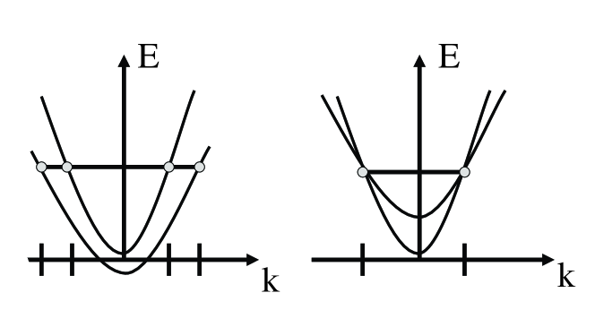
Figure 1: Relation dispersion $E(k)$ for a system with spin dependent hopping. Left: in the traditional case there are spin relaxation phenomena ensuring the equilibrium of the two spin species. There is thus a unique chemical potential for both species. This implies the presence of four fermi points. Right: for cold atoms, there is no such relaxation and the number of spin up and down are separately conserved. For an equal number of spin up and down, there is thus only two Fermi points since the two fermi momenta ${k_{F}}_{\uparrow}={k_{F}}_{\downarrow}$.

For such a system, the various operators corresponding to the different types of order in the tubes are of two types[1]. There are charge density or spin density order described by

$$O_{\rho}(x) = \sum_{\sigma,\sigma^{\prime}}\psi^{\dagger}_{\sigma}(x)\delta_{\sigma,\sigma^{\prime}}\psi^{\vphantom{\dagger}}_{\sigma^{\prime}}(x)$$ (2)

$$O_{\sigma}^{a}(x) = \sum_{\sigma,\sigma^{\prime}}\psi^{\dagger}_{\sigma}(x)\sigma^{a}_{\sigma,\sigma^{\prime}}\psi^{\vphantom{\dagger}}_{\sigma^{\prime}}(x)$$ (3)

where $\sigma^{x}$, $\sigma^{y}$, $\sigma^{z}$ are the Pauli matrices The operator $O_{\rho}$ is simply the total density, whereas $O_{\sigma}^{a}(x)$ measures the spin density (along the direction $a=x,y,z$). We have used the notation in the continuum $c_{m}\to\psi(x)$ as the operator destroying a fermion at point $x$. The density contains a $q\sim 0$ component and a $q\sim 2k_{F}$ one. The operators giving the $2k_{F}$ modulation of the charge or spin density are

$$O_{{\rm CDW}}(x) = \psi^{\dagger}_{R\uparrow}\psi^{\vphantom{\dagger}}_{L\uparrow}(x)+\psi^{\dagger}_{R\downarrow}\psi^{\vphantom{\dagger}}_{L\downarrow}(x)=\frac{e^{-2ik_{F}x}}{\pi\alpha}e^{i\sqrt{2}\phi_{\rho}}\cos(\sqrt{2}\phi_{\sigma})$$ (4)

$$O_{{\rm SDW}}^{x}(x) = \psi^{\dagger}_{R\uparrow}\psi^{\vphantom{\dagger}}_{L\downarrow}(x)+\psi^{\dagger}_{R\downarrow}\psi^{\vphantom{\dagger}}_{L\uparrow}(x)=\frac{e^{-2ik_{F}x}}{\pi\alpha}e^{i\sqrt{2}\phi_{\rho}}\cos(\sqrt{2}\theta_{\sigma})$$ (5)

$$O_{{\rm SDW}}^{y}(x) = -i(\psi^{\dagger}_{R\uparrow}\psi^{\vphantom{\dagger}}_{L\downarrow}(x)-\psi^{\dagger}_{R\downarrow}\psi^{\vphantom{\dagger}}_{L\uparrow}(x))=\frac{-e^{-2ik_{F}x}}{\pi\alpha}e^{i\sqrt{2}\phi_{\rho}}\sin(\sqrt{2}\theta_{\sigma})$$ (6)

$$O_{{\rm SDW}}^{z}(x) = \psi^{\dagger}_{R\uparrow}\psi^{\vphantom{\dagger}}_{L\uparrow}(x)-\psi^{\dagger}_{R\downarrow}\psi^{\vphantom{\dagger}}_{L\downarrow}(x)=\frac{e^{-2ik_{F}x}}{\pi\alpha}e^{i\sqrt{2}\phi_{\rho}}i\sin(\sqrt{2}\phi_{\sigma})$$ (7)

where we have used the notation $\psi^{\dagger}_{R}$ (resp. $\psi^{\dagger}_{L}$) to denote the operator creating a fermion with a momentum close to $+k_{F}$ (resp. $-k_{F}$). These operators have a simple representation in terms of continuous field $\phi_{\rho,\sigma}$ (resp. $\theta_{\rho,\sigma}$) describing the collective excitations of charge and spin densities (resp. current densities). This representation is the so-called bosonization representation and is very useful to identify the types of order in the system. For more details on this representation see e.g. Ref. giamarchi_book_1d. Here we will only use that $\phi$ and $\nabla\theta$ have canonical conjugation commutation relations, so order in one of the field implies exponentially decreasing correlations in the other. Besides the above mentioned types of order, other instability in the system are the superfluid instabilities of the singlet or triplet type

$$O_{\SS}(x) = \sum_{\sigma,\sigma^{\prime}}\sigma\psi^{\dagger}_{R,\sigma}(x)\delta_{\sigma,\sigma^{\prime}}\psi^{\dagger}_{L,-\sigma^{\prime}}(x)$$ (8)

$$O_{{\rm TS}}^{a}(x) = \sum_{\sigma,\sigma^{\prime}}\sigma\psi^{\dagger}_{R,\sigma}(x)\sigma^{a}_{\sigma,\sigma^{\prime}}\psi^{\dagger}_{L,-\sigma^{\prime}}(x)$$ (9)

where SS denotes singlet pairing whereas TS is triplet pairing. These operators describe paring with zero total momentum. Other pairings are of course possible but are usually less relevant. These operators become

$$O_{\SS}(x) = \psi^{\dagger}_{R\uparrow}\psi^{\dagger}_{L\downarrow}(x)+\psi^{\dagger}_{L\uparrow}\psi^{\dagger}_{R\downarrow}(x)=\frac{1}{\pi\alpha}e^{-i\sqrt{2}\theta_{\rho}}\cos(\sqrt{2}\phi_{\sigma})$$ (10)

$$O_{{\rm TS}}^{x}(x) = \psi^{\dagger}_{R\uparrow}\psi^{\dagger}_{L\uparrow}(x)+\psi^{\dagger}_{L\downarrow}\psi^{\dagger}_{R\downarrow}(x)=\frac{1}{\pi\alpha}e^{-i\sqrt{2}\theta_{\rho}}\cos(\sqrt{2}\theta_{\sigma})$$ (11)

$$O_{{\rm TS}}^{y}(x) = -i(\psi^{\dagger}_{R\uparrow}\psi^{\dagger}_{L\uparrow}(x)-\psi^{\dagger}_{L\downarrow}\psi^{\dagger}_{R\downarrow}(x))=\frac{-1}{\pi\alpha}e^{-i\sqrt{2}\theta_{\rho}}\sin(\sqrt{2}\theta_{\sigma})$$ (12)

$$O_{{\rm TS}}^{z}(x) = \psi^{\dagger}_{R\uparrow}\psi^{\dagger}_{L\downarrow}(x)-\psi^{\dagger}_{L\uparrow}\psi^{\dagger}_{R\downarrow}(x)=\frac{e^{2ik_{F}x}}{\pi\alpha}e^{-i\sqrt{2}\theta_{\rho}}\sin(\sqrt{2}\phi_{\sigma})$$ (13)

We will not dwell on the solution[10] of the model here and will only quote the results. Compared to the standard case of the Hubbard model the main effect of the spin dependent hopping is to open a spin gap both for repulsive and attractive interactions (the standard Hubbard model being massless for repulsive interactions). For attractive interactions the spin gap corresponds to the formation of singlets. In the bosonization language this corresponds to the order $\phi_{\sigma}\to 0$. Correlation functions containing $\theta_{\sigma}$ or $\sin(\sqrt{2}\phi_{\sigma})$ thus decay exponentially to zero. The leading instabilities are thus the charge density wave (CDW) order or a singlet superfluid (SS) instability. Physically it means that fermions of opposite spin pair and that these pairs behave roughly as bosons and can then condense to give a superfluid (SS) or crystallize to give a charge density wave (CDW).

For repulsive interactions the hopping difference induce an order in $\phi_{\sigma}\to\pi/\sqrt{8}$. Correlation functions containing $\theta_{\sigma}$ or $\cos(\sqrt{2}\phi_{\sigma})$ decay exponentially to zero while $\sin(\sqrt{2}\phi_{\sigma})$ tends to a constant. The leading instabilities are thus a spin density wave order along the $z$ direction (${\rm SDW}_{z}$) or a triplet superfluid instability along $z$ ($TS_{z}$). Which one of these instabilities dominates is dictated by the decay of the correlations of the charge sector that remains massless. For repulsive interactions, the ${\rm SDW}_{z}$ one dominates, while the ${\rm TS}_{z}$ one decays with a larger power law and is thus subdominant. A summary of the phase diagram is given in Fig. 2.

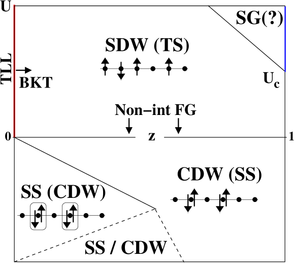
Figure 2: Schematic phase diagram for the model in Eq. (1) with equal number of spin up and down fermions away from half-filling. The interaction strength is $U$ and $z=|t_{\uparrow}-t_{\downarrow}|/(t_{\uparrow}+t_{\downarrow})$. All phases (SDW: spin density wave, CDW: charge density wave, SS singlet superfluid, TS triplet superfluid) exhibit a spin gap $\Delta_{s}$ (however, $\Delta_{s}=0$ for $U=0$ and $z=0$ with $U>0$. A cartoon of the type of order characterizing each phase is also shown. In the area between dashed lines the dominant order (either CDW or SS) depends on the lattice filling. In the SG phase, spin up and down fermions are segregated (demixed).

For repulsive interactions the spin sector is thus still massive but the spin gap does not correspond to the formation of singlets. On the contrary it is due to a breaking of the spin rotation symmetry with formation of an ising-like antiferromagnetic order along the $z$ direction. Note that even if the spin sector is massive, the spin density wave order is not perfect (except at a commensurate filling of exactly one fermion per site) due to the fluctuations in the charge sector. Contrarily to the case of the Hubbard model where the SDW order in the three directions decays in a similar way (due to the spin rotation symmetry) here the SDW_z order decays as a power law because of charge fluctuations while SDW_x,y order decays exponentially fast because of the presence of the gap in the spin sector. We refer the reader to Ref. cazalilla_fermions_1d for more details on the various correlation functions and ways to probe the existence of such a gap by Raman spectroscopy.

3 Coupled Fermionic tubes

Let us now turn to the case of coupled tubes. The coupling between the tubes can be described by the single particle hopping term

$$H_{\perp}=-t_{\perp}\sum_{\langle\alpha,\beta\rangle}\sum_{m,\sigma}c^{\dagger}_{\sigma,m,\alpha}c_{\sigma,m,\beta}$$ (14)

where $\alpha$ and $\beta$ are the tube indexes and $\langle\alpha,\beta\rangle$ denotes nearest neighbor tubes. Because for cold atomic gases the interactions are short range, there is no need to take into account interactions between different tubes. If the single particle hopping (14) is of the same order of magnitude than the ones in (1) then the system is a three dimensional system, while if $t_{\perp}=0$ the tubes are uncoupled. The Hamiltonian (14) is thus able to describe the dimensional crossover between these two situations. For bosons the effects of such a term have been investigated in Ref. ho_deconfinement_coldatoms. For fermions treating such a single particle hopping is an extremely challenging problem. Indeed, contrarily to the case of boson, the average of a single fermion operator does not exist, and thus the term (14) cannot be decoupled simply. Various approximations have thus been used to tackle this term and we refer the reader to Ref. biermann_oned_crossover_review,giamarchi_review_chemrev,giamarchi_book_1d for details and further references.

However for the particular case of the fermionic system investigated in these notes, one is in a much more favorable situation because of the presence of the spin gap. In the case of attractive interactions, the fermions form singlet pairs, that essentially behave as bosons. One is thus essentially led back to the bosonic case of Ref. ho_deconfinement_coldatoms. We thus focus here on the more interesting repulsive case. Because of the presence of the spin gap the situation is now quite different to the one where each tube is described by the simple Hubbard model. In the latter case the spin excitations are massless and the single particle correlations decay as power laws

$$\langle T_{\tau}c_{\alpha,\sigma,}(x)c^{\dagger}_{\alpha,\sigma}(0)\rangle\propto\left(\frac{1}{x}\right)^{\frac{1}{4}[K_{\rho}+1/K_{\rho}]+\frac{1}{2}}$$ (15)

where $K_{\rho}$ is an interaction dependent parameter (the Luttinger liquid parameter) characterizing the isolated tube. In that case a simple scaling analysis to second order in perturbation in the single particle hopping term (14) shows that it scales as

$$t_{\perp}^{2}L^{4-\frac{1}{2}[K_{\rho}+1/K_{\rho}]-1}$$ (16)

and is thus in general a relevant perturbation, driving the system away from the isolated tube fixed point. However in the presence of a spin gap the single particle excitations now decay exponentially

$$\langle T_{\tau}c_{\alpha,\sigma,}(x)c^{\dagger}_{\alpha,\sigma}(0)\rangle\propto e^{-|x|/\xi}$$ (17)

where $\xi$ is the correlation length induced by the presence of the spin gap (typically of order $\xi=v_{F}/\Delta_{s}$ if $v_{F}$ is the Fermi velocity). The single particle hopping is now an irrelevant perturbation to (1). Physically it simply means that because of the presence of the spin gap it is now impossible for a single particle to leave a tube since it would take away one spin and thus destroy the spin gap. One would therefore need a critical value of $t_{\perp}$ for this to happen. However, although the single particle hopping is an irrelevant operator, it can generate relevant perturbations at higher order[1]. Such relevant perturbations corresponds to hopping between different tubes that do not destroy the spin gap.

Quite generally, as shown in Fig. 3, two types of relevant perturbations are possible when looking at the second order term generated by (14).

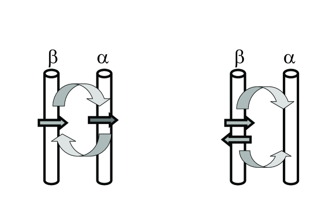
Figure 3: Relevant coupling generated to second order by the single particle intertube hopping. In order to avoid breaking the spin gap, a correlated hop of two objects must be done simultaneously. Left: particle-hole hopping. Since this term exchanges two particles on two different tubes, it corresponds to a standard density-density or spin-spin coupling term. This is the superexchange term. Right: particle-particle hopping. This term allows a pair to jump from one tube to the next and is thus analogous to the Josephson coupling between superconductors.

The first one corresponds to particle-hole hopping between the tubes, it is thus a density-density or spin-spin term, while the second one is the hopping of two particles between between the tubes and thus corresponds to a Josephson coupling. The simplest way to analyze the terms generated by (14) is to use the bosonization representation. The intertube tunnelling term becomes

$$H_{\perp} \propto -t_{\perp}\sum_{\sigma=\pm 1,r=\pm 1}\sum_{\langle\alpha,\beta\rangle}\int dxe^{\frac{i}{\sqrt{2}}[r\phi_{\rho,\alpha}(x)-\theta_{\rho,\alpha}(x)+s(r\phi_{\sigma,\alpha}(x)-\theta_{\sigma,\alpha}(x))]}\times$$ (18)

$$e^{\frac{-i}{\sqrt{2}}[r\phi_{\rho,\beta}(x)-\theta_{\rho,\beta}(x)+s(r\phi_{\sigma,\beta}(x)-\theta_{\sigma,\beta}(x))]}$$

Going to second order in (14), using the fact that $\phi_{\sigma}$ is now ordered, and the fact that all operators leading to exponential decay must be eliminated to get the leading operator, one sees that a first surviving term is

$$H_{{\rm SDW}}=J_{{\rm SDW}}\sum_{\alpha,\beta}\int dxO_{{\rm SDW}_{z},\alpha}^{\dagger}(x)O_{{\rm SDW}_{z},\beta}(x)$$ (19)

The value of the coupling constant can be obtained by standard second order perturbation theory and is of the order of $J_{{\rm SDW}}\sim t_{\perp}^{2}/\Delta_{s}$. This term is thus a standard superexchange term coupling the antiferromagnetic spin modulation on two different tubes. Quite naturally this term would tend to stabilize the ${\rm SDW}_{z}$ instability that would develop in an isolated tube and lead to a three dimensional ordered antiferromagnetic phase.

There is however another term that survives. This is a term where two particles can hop from one tube to the other. It is of the form

$$H_{{\rm TS}}=J_{{\rm TS}}\sum_{\alpha,\beta}\int dxO_{{\rm TS}_{z},\alpha}^{\dagger}(x)O_{{\rm TS}_{z},\beta}(x)$$ (20)

This term corresponds to the hopping of a pair of fermions, that are in a triplet paring state from one tube to the other. Singlet hopping is here cancelled because of the presence of the spin gap. Because a superfluid pair has a global momentum of zero, the pair hopping does not contain the oscillating $2k_{F}$ factor that is present in the superexchange term (see (4)). Here again the coupling constant is of the order of $J_{{\rm TS}}\sim t_{\perp}^{2}/\Delta_{s}$.

Both the superexchange and the Josephson term tend to stabilize their corresponding type of order. What phase is realized normally depends crucially on what is the leading one dimensional instability. Usually the Fermi momenta of all tubes are the same and there is no oscillatory factors in (19). Since the ${\rm SDW}$ order is dominant for the isolated tube, and both $J_{\rm SDW}$ and $J_{\rm TS}$ are of the same order of magnitude a simple RPA treatment of the coupling term shows that the ${\rm SDW}$ phase is stabilized. This is the situation depicted in Fig. 4(a). This situation is normally the one realized in condensed matter systems. It corresponds to the stabilization of a three dimensional antiferromagnetic order for repulsive interactions. However the situation can be much richer if the Fermi momenta of the different tubes are different. Note that for cold atoms this is the rule rather than the exception because of the presence of the parabolic confining potential that makes each tube different depending from its distance from the center. This situation can also be reinforced artificially by adding an additional modulation of the optical lattice. In that case one has $k_{F}^{\alpha}-k_{F}^{\beta}\neq 0$ which means that the oscillatory factors remain in (19). Such factors considerably weaken the intertube superexchange. Physically this means that the antiferromagnetic fluctuations on the neighboring tubes are now incommensurate with each other and thus cannot couple very well as depicted in Fig. 4(b). On the other hand the Josephson term which is a $q\sim 0$ transfer between the tube is not affected by such a difference of Fermi momentum and remains unchanged, as schematically shown in Fig. 4(c). One is now in a situation where this term can become dominant[10] even if the triplet superfluid instability in the isolated tube is a subdominant instability. One would thus be in a situation to stabilize a three dimensional triplet superfluid phase.

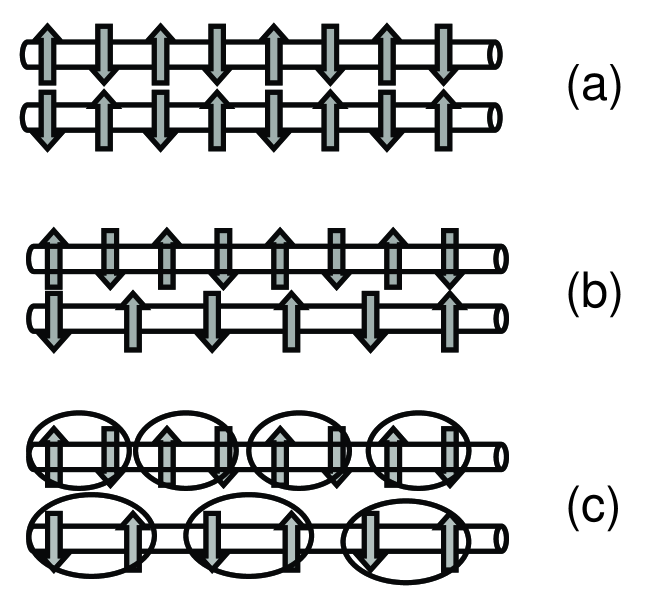
Figure 4: Schematic diagrams for the true long range order induced by inter-tube particle-pair or particle-hole hopping. a) Antiferromagnetic order for $U>0$ and different velocities, with equal Fermi momentum (i.e. equal number of fermions in each tube). b) Frustration (incommensurability) to the antiferromagnetic order between tubes when the Fermi momentum is different between the tubes. c) No such frustration effects when the order parameter carries zero total momentum, namely for the superfluidity.

This is a rather unique situation. From the theoretical point of view such a stabilization of a subdominant instability by intertube coupling is quite interesting and potentially relevant to other situations as well. In particular, this mechanism is similar, albeit for a triplet superconductor, to the one advocated to stabilize singlet superconductivity for coupled stripes[12]. Such cold atomics system could thus be controlled systems in which to check for the feasibility of such a mechanism. More directly it would be very interesting to have a realization for a triplet superconductor. Triplet superconductivity is indeed quite rare. Besides Helium 3, strontium ruthenate is the only one candidate well identified in condensed matter[13]. Organic superconductors, another system made of coupled chains, is also a potential candidate for such unusual superconductivity[14]. Cold atomic gases of fermions could thus help shed a light on the mechanisms and properties of unusual superconductivity in these very anisotropic systems.

References

- [1] T. Giamarchi, Quantum Physics in One Dimension (Oxford University Press, Oxford, 2004).
- [2] M. Greiner et al., Nature 415, 39 (2002).
- [3] T. Stöferle et al., Phys. Rev. Lett. 92, 130403 (2004).
- [4] S. Inouye et al., Nature 392, 151 (1998).
- [5] E. Timmermans, K. Furuya, P. W. Milonni, and A. K. Kerman, Phys. Lett. A 258, 228 (2001).
- [6] M. Holland, S. J. J. M. F. Kokkelmans, M. L. Chiofalo, and R. Walser, Phys. Rev. Lett. 87, 120406 (2001).
- [7] T. Giamarchi, Chem. Rev. 104, 5037 (2004).
- [8] A. F. Ho, M. A. Cazalilla, and T. Giamarchi, Phys. Rev. Lett. 92, 130405 (2004).
- [9] M. Kohl et al., Phys. Rev. Lett. 94, 080403 (2005).
- [10] M. A. Cazalilla, A. F. Ho, and T. Giamarchi, Phys. Rev. Lett. 95, 226402 (2005).
- [11] S. Biermann, A. Georges, T. Giamarchi, and A. Lichtenstein, in Strongly Correlated Fermions and Bosons in Low Dimensional Disordered Systems, edited by I. V. Lerner et al. (Kluwer Academic Publishers, Dordrecht, 2002), p. 81, cond-mat/0201542.
- [12] E. Arrigoni, E. Fradkin, and S. Kivelson, Phys. Rev. B 69, 214519 (2004).
- [13] A. P. Mackenzie and Y. Maeno, Rev. Mod. Phys. 75, 657 (2003).
- [14] T. Ishiguro, in High Magnetic Fields: Applications in Condensed Matter Physics and Spectroscopy, Vol. 595 of Lecture Notes in Physics, edited by C. Berthier, L. P. Lévy, and G. Martinez (Springer-Verlag, Heidelberg, 2002), pp. 301–313.