A quantitative study of spin noise spectroscopy in a classical gas of ⁴¹K atoms

Abstract

We present a general derivation of the electron spin noise power spectrum in alkali gases as measured by optical Faraday rotation, which applies to both classical gases at high temperatures as well as ultracold quantum gases. We show that the spin-noise power spectrum is determined by an electron spin-spin correlation function, and we find that measurements of the spin-noise power spectra for a classical gas of ⁴¹K atoms are in good agreement with the predicted values. Experimental and theoretical spin noise spectra are directly and quantitatively compared in both longitudinal and transverse magnetic fields up to the high magnetic field regime (where Zeeman energies exceed the intrinsic hyperfine energy splitting of the ⁴¹K ground state).

I Introduction

In general, the magnitude of the measured response of a system to an external perturbation decreases as the size of the system decreases, and therefore conventional probes based on the measurement of linear response often become impractical for the study of nanosystems. However, the fluctuation-dissipation theorem Kubo guarantees that the linear response of a system can also be determined from the spectrum of the system’s internal fluctuations while in equilibrium. To probe the intrinsic fluctuations of a system one can use any of a variety of so-called ‘noise spectroscopies’, which typically disturb the system much less as compared with measurements based on intentional perturbation of the system Aleksandrov ; Sleator ; Awschalom ; Weissman ; Sorensen ; Kuzmich ; Smith ; Mitsui ; Ito ; ref:spin ; Oestreich . Further, fluctuation signals generally offer more advantageous scaling with size as the system size is reduced Mamin ; ref:spin .

Recently, we utilized a noise spectroscopy based on ultrasensitive magneto-optical Faraday rotation applied to classical gases of alkali atoms ref:spin with an aim to measure the spectrum of intrinsic spin (magnetization) fluctuations in an atomic ensemble. In this experiment a linearly polarized laser, detuned from one of the fundamental s-p (D1 or D2) optical transitions of the alkali atom, was transmitted through the alkali vapor (which itself was in thermal equilibrium). To leading order, the laser detuning was sufficiently large to ensure no absorption of the laser by the atoms, and so the laser was primarily sensitive to the dispersive (real) part of the atomic dielectric function through the vapor’s spin-sensitive index of refraction Happer . Stochastic spin fluctuations in the alkali ensemble therefore imparted small fluctuations in the polarization rotation (Faraday rotation) angle of the transmitted laser. These Faraday rotation angle fluctuations, measured as a function of time, exhibited power spectra showing clear noise resonances at frequencies corresponding to the differences between the various hyperfine/Zeeman atomic levels of the alkali atom. The experiments in Ref. ref:spin were performed at relatively high temperatures, where the alkali atoms behave as a classical Boltzmann gas and interatomic interactions are unimportant. In addition, these experiments were conducted in the low magnetic field regime where Zeeman energies were much less than the typical hyperfine splittings of the atomic ground state. From the spin noise spectra alone and with the atomic ensemble remaining in thermal equilibrium, a determination of the atomic g-factors, nuclear spin, isotope abundance ratios, hyperfine splittings, nuclear moments and spin coherence lifetimes was possible. These properties of classical alkali atoms are, of course, already well known Corney ; the experiments described in Ref. ref:spin established the practical value of spin noise spectroscopy for determining the properties of atomic gases and the magnitude of spin noise signals expected under various experimental conditions.

We have also recently suggested us that this type of spin noise spectroscopy is a promising experimental probe for ultracold alkali atomic gases because: i) it is only weakly perturbing and, ii) based on the classical alkali gas measurements, large noise signals are expected. Ultracold gases of alkali atoms anderson ; davis ; bradley ; demarco provide experimentally accessible model systems for probing quantum states that manifest themselves at the macroscopic scale. Because the temperature is very low, interactions between the alkali atoms are important, and novel many-body quantum states arise because of these interactions. The ability to vary the effective interatomic interaction (by varying an external magnetic field and thus adjusting the relative strength of the hyperfine and Zeeman interactions) makes ultracold atom gases especially interesting model systems for a wide range of quantum many-body systems. The properties of ultracold gases of alkali atoms are of great interest and are just beginning to be understood. New experimental probes of these systems aimed at revealing the underlying interatomic interactions will be very useful.

Faraday rotation in alkali gases is sensitive to the projection of the atom’s electron spin in the direction of laser propagation Aleksandrov ; Kuzmich ; Happer . In general, projections of electron spin alone are not good quantum numbers of the alkali atom Hamiltonian. At low magnetic fields where the Zeeman energies are smaller than or comparable to the hyperfine interaction, the electron and nuclear spins are entangled and no projection of electron spin is a good quantum number. At strong magnetic fields where the Zeeman splitting is much larger than the hyperfine splitting, the electron spin projection in the direction of the magnetic field becomes a good quantum number, but electron spin projection orthogonal to the magnetic field is not. Thus, noise spectroscopy at low temperature can be performed with the magnetic field either parallel or orthogonal to the direction of laser propagation whereas in the high-field limit, the magnetic field should be orthogonal to the direction of laser propagation.

In this paper, we derive a general expression for the spin noise power spectrum in alkali gases as measured by optical Faraday rotation and show that the noise power spectrum is determined by an electron spin-spin correlation function. This general expression applies to both classical gases at high temperature as well as ultracold quantum gases. We make detailed calculations of the expected noise spectra for a classical gas of ⁴¹K atoms and compare these calculated results with quantitative measurements of the spin noise power. We find good agreement between the calculated and measured results in both the low- and high-magnetic field limit. Isotopically enriched alkali vapors of ⁴¹K were chosen because the relatively small hyperfine splitting of this atom ($\sim$254 MHz) allows to approach the high-field limit rather easily (magnetic fields of order 100 Gauss).

The paper is organized as follows: In Sec. II we derive the general expression for the spin noise power spectrum as measured by Faraday rotation. In Sec. III we consider the specific case of a classical gas of ⁴¹K atoms and calculate the expected noise spectra. In Sec. IV we present experimental results of spin-noise measurements on a classical gas of ⁴¹K atoms, and compare with our theoretical results. We present our conclusions in Sec. V.

II Response function for spin noise spectroscopy

The experimental arrangement for Faraday rotation measurements of spin noise is shown schematically in Fig. 1. A linearly polarized laser, detuned from a s-p (D1 or D2) atomic transition of the alkali atoms, traverses a cell containing the atomic gas. A magnetic field is applied either perpendicular (as shown in Fig. 1) or parallel to the laser propagation direction. After traversing the atomic gas the laser beam is divided by a beam splitter at 45^∘ to the original polarization direction. The split optical beams are detected by a pair of matched photodiodes and the difference signal (proportional to Faraday rotation, which is proportional to the magnetization of the alkali ensemble) is analyzed by a spectrum analyzer. Full experimental details are given in Section IV.

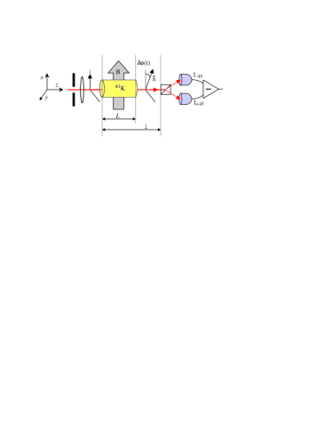
Figure 1: (Color online) Experimental schematic showing how electron spin noise in a classical vapor of ⁴¹K atoms is probed via optical Faraday rotation. Spin fluctuations in the vapor impart Faraday rotation fluctuations $\delta\phi(t)$ on a linearly-polarized and detuned laser beam, which are measured in a sensitive optical bridge. The external magnetic field can be applied orthogonal to (as shown) or parallel to the direction of laser propagation.

In the electronic ground state of alkali atoms (s-orbital) there is a strong hyperfine coupling between the nuclear and electron spins. For the electronic p-orbital the hyperfine splitting is weak because the p-orbital has a node at the nuclear position, however there is a strong spin-orbit coupling between the p-orbital and its spin. Photons directly couple to the spatial part of the electron wave function, but because of the spin-orbit splitting in the final state of the optical transition there is an indirect coupling between the photons and the electron spin. A fluctuating birefringence, that is a difference in refractive index for left and right hand circular polarizations, results from fluctuations in the electron spin and leads to a fluctuating Faraday rotation $\delta\phi(t)$ of the transmitted laser. The experiment is therefore sensitive to fluctuations of electron spin projection in the direction of laser propagation.

The polarization rotation angle noise is

$$\frac{\phi_{N}(\omega)}{\sqrt{\delta f}}=\ \Bigl{[}P(\omega)\Bigr{]}^{1/2}\>,$$ (1)

where the noise power is

$$P(\omega)=\ \int\mathrm{d}t\ e^{\mathrm{i}\omega t}\ \langle\delta\phi(t)\,\delta\phi(0)\rangle\>.$$ (2)

The optical field is characterized by the vector potential at position $\mathbf{r}$, which we can write as

$$\mathbf{A}(\mathbf{r},t)=\ \mathbf{a}_{0}(\mathbf{r},t)\ +\ \sum_{k}\ \mathbf{\delta a}_{k}(\mathbf{r},t)\>,$$ (3)

where

$$\mathbf{a}_{0}(\mathbf{r},t)=\ \mathbf{A}_{0}\ F(\mathbf{r})\ e^{\mathrm{i}\frac{\Omega}{c}(z-ct)}\>,$$ (4)

is the incident laser beam and

$$\mathbf{\delta a}_{k}(\mathbf{r},t)=\ \mathbf{A}_{0}\cdot\tilde{a}_{k}(\Omega,\theta)\ F(\mathbf{r}_{k})\ e^{\mathrm{i}\frac{\Omega}{c}z_{k}}\ \frac{e^{\mathrm{i}\frac{\Omega}{c}\bigl{(}|\mathbf{r}-\mathbf{r}_{k}|-ct\bigr{)}}}{|\mathbf{r}-\mathbf{r}_{k}|}\>$$ (5)

is the scattered optical beam. Here, $F(\mathbf{r})$ is the beam profile, normalized to unity in the cross-section plane orthogonal to the direction of the incident beam, $\hat{z}$, i.e.

$$1= \int\mathrm{d}^{2}\rho\ |F(\mathbf{r})|^{2}\>,\qquad\mathrm{with}\ \mathbf{r}=(\vec{\rho},z)\>.$$ (6)

We denote by $\theta$, the scattering angle between $\hat{z}$ and $(\mathbf{r}-\mathbf{r}_{k})$, the position of the atom $k$ and the point $\mathbf{r}$. We introduced $\mathbf{A_{0}}=A_{0}\,\hat{\epsilon}$, where $A_{0}$ is a strength parameter and $\hat{\epsilon}=\hat{x}$ is the linear polarization of the incident beam. The scattering amplitude matrix is

$$\tilde{a}^{\mathrm{in},\,\mathrm{out}}(\Omega,\theta)=\ \frac{r_{0}}{m_{0}}\,\frac{1}{\hbar}\,\frac{(\mathbf{P}\cdot\hat{\epsilon}_{\mathrm{in}}^{*})\,\mathcal{P}_{J}\,(\mathbf{P}\cdot\hat{\epsilon}_{\mathrm{out}}^{*})}{\Omega_{J\,R}-\Omega}\>,$$ (7)

where $\Omega$ is the angular frequency of the laser, $r_{0}=e^{2}/(mc^{2})$ is the classical electron radius, $m_{0}$ is the electron mass, $\mathbf{P}$ is the electron momentum operator, $\mathcal{P}_{J}=\Sigma|J\rangle\langle J|$ is the projection operator on to the near-resonant set of intermediate state, $\{|J\rangle\}$, and $\Omega_{J\,R}$ is the atomic resonance angular frequency. In Eq. (3) we have assumed that $|\mathbf{\delta a}_{k}(\mathbf{r},t)|\ll|\mathbf{a}_{0}(\mathbf{r},t)|$, i.e. we work in the weak scattering limit.

The polarization beamsplitter forms two beams with intensities

$$I_{\pm}(\mathbf{r})=\ |\mathbf{A}(\mathbf{r},t)\cdot\hat{\epsilon}_{\pm}|^{2}\>,$$ (8)

and linear polarizations

$$\hat{\epsilon}_{\pm}=\ \frac{1}{\sqrt{2}}\ (\hat{x}\pm\hat{y})\>.$$ (9)

The difference of the two beam intensities in the weak scattering approximation is

$$I_{+}(\mathbf{r})\ -\ I_{-}(\mathbf{r})$$ (10)

$$=\ 2\,\bigl{[}\mathbf{a}_{0}(\mathbf{r},t)\cdot\hat{\epsilon}_{\pm}\bigr{]}^{*}\ \bigl{[}\mathbf{\delta a}(\mathbf{r},t)\cdot(\hat{\epsilon}_{+}-\,\hat{\epsilon}_{-})\bigr{]}$$

with the components of the vector potential $\mathbf{A}(\mathbf{r},t)$ evaluated in the forward scattering direction (Eq. (3), with $\theta=0$). Then

$$\mathbf{a}_{0}(\mathbf{r},t)\cdot\hat{\epsilon}_{\pm}=\ \frac{1}{\sqrt{2}}\ A_{0}\ F(\mathbf{r})\ e^{\mathrm{i}\frac{\Omega}{c}(z-ct)}\>,$$ (11)

where $\mathbf{a}_{0}(\mathbf{r},t)\cdot\hat{\epsilon}_{+}=\mathbf{a}_{0}(\mathbf{r},t)\cdot\hat{\epsilon}_{-}$, and

$$\mathbf{\delta a}(\mathbf{r},t)\,\cdot\, (\hat{\epsilon}_{+}-\,\hat{\epsilon}_{-})=\ A_{0}\,\sum_{k}\,F(\mathbf{r}_{k})\ e^{\mathrm{i}\frac{\Omega}{c}z_{k}}\$$ (12)

$$\times\,\Bigl{[}\hat{\epsilon}\cdot\tilde{a}_{k}(\Omega,0)\cdot(\hat{\epsilon}_{+}-\hat{\epsilon}_{-})\Bigr{]}\ \frac{e^{\mathrm{i}\frac{\Omega}{c}\bigl{(}|\mathbf{r}-\mathbf{r}_{k}|-ct\bigr{)}}}{|\mathbf{r}-\mathbf{r}_{k}|}\>.$$

The photodiode bridge measures the difference of the two intensities integrated over the laser spot at the detection plane. The integrated intensity difference measured in a cross-section plane, $\mathcal{I}$, is

$$\mathcal{I}\equiv\int\mathrm{d}^{2}\rho\ \bigl{[}I_{+}(\mathbf{r},t)-I_{-}(\mathbf{r},t)\bigr{]}$$ (13)

$$=\ -\mathrm{i}\,A_{0}^{2}\ \sum_{k}\,F(\mathbf{r}_{k})\ e^{\mathrm{i}\frac{\Omega}{c}(z_{k}-z)}\,\Bigl{[}\tilde{a}_{k}^{LL}(\Omega,0)-\tilde{a}_{k}^{RR}(\Omega,0)\Bigr{]}$$

$$\qquad\times\,\int\mathrm{d}^{2}\rho\ F(\vec{\rho},z)^{*}\ \frac{e^{\mathrm{i}\frac{\Omega}{c}|\mathbf{r}-\mathbf{r}_{k}|}}{|\mathbf{r}-\mathbf{r}_{k}|}\>$$

with $\mathbf{r}$ evaluated on the detection plane. Here, $\tilde{a}^{LL}$ and the $\tilde{a}^{RR}$ denote the diagonal elements of the scattering amplitude matrix $\tilde{a}$ in the circular polarization basis,

$$\hat{\epsilon}_{L,R}=\ \frac{1}{\sqrt{2}}\ (\hat{x}\pm\mathrm{i}\,\hat{y})\>.$$ (14)

In the circular polarization basis, we have:

$$\hat{\epsilon}_{+}-\hat{\epsilon}_{-}= \ -\mathrm{i}\ (\hat{\epsilon}_{L}-\hat{\epsilon}_{R})\>,$$ (15)

$$\hat{\epsilon}= \ \frac{1}{\sqrt{2}}\ (\hat{\epsilon}_{L}+\hat{\epsilon}_{R})\>.$$ (16)

At the detection plane, at $z=\ell$, the $\vec{\rho}$ integral in Eq. (13) gives

$$\int\mathrm{d}^{2}\rho\ F(\vec{\rho},\ell)^{*} \ \frac{e^{\mathrm{i}\frac{\Omega}{c}\sqrt{|\vec{\rho}-\vec{\rho}_{k}|^{2}+(\ell-z_{k})^{2}}}}{\sqrt{|\vec{\rho}-\vec{\rho}_{k}|^{2}+(\ell-z_{k})^{2}}}$$ (17)

$$\approx\ 2\pi\,\mathrm{i}\ \frac{c}{\Omega}\ e^{\mathrm{i}\frac{\Omega}{c}(\ell-z_{k})}\ F(\mathbf{r}_{k})^{*}\>,$$

where we have assumed that $(\ell-z_{k})^{2}\gg(\rho-\rho_{k})^{2}$, and $F(\mathbf{r}_{k})$ is slowly varying on the scale of the optical wavelength. Thus, we obtain

$$\mathcal{I}=\ \frac{2\pi c}{\Omega}\ A_{0}^{2}\ \sum_{k}\ |F(\mathbf{r}_{k})|^{2}\,\Bigl{[}\tilde{a}_{k}^{LL}(\Omega,0)-\tilde{a}_{k}^{RR}(\Omega,0)\Bigr{]}\>,$$ (18)

with

$$\tilde{a}^{LL}(\Omega,0)-\,\tilde{a}^{RR}(\Omega,0)=\ \pm\frac{2r_{0}}{3m_{0}}\,\frac{1}{\hbar}\ \frac{|\langle S|p_{x}|P_{x}\rangle|^{2}}{|\Omega_{J\,R}-\Omega|}\ \sigma_{z}\>.$$ (19)

Here, $<S|p_{x}|P_{x}>$ is the momentum matrix element for the optical transition, $\hat{z}$ is the direction of laser propagation, and the $\pm$ correspond to the resonances $|J\rangle=|L+\frac{1}{2};I\rangle$ and $|J\rangle=|L-\frac{1}{2};I\rangle$ states with $L=1$, respectively. We obtain

$$\mathcal{I}=\ \pm\, \frac{4\pi}{3}\,\frac{cr_{0}}{m_{0}}\,\frac{1}{\hbar\Omega}\ A_{0}^{2}\ \frac{|\langle S|p_{x}|P_{x}\rangle|^{2}}{\Omega_{J\,R}-\Omega}$$

$$\times\int\mathrm{d}^{3}R\ |F(\mathbf{R})|^{2}\ \sigma_{z}(\mathbf{R})\>.$$ (20)

where $\sigma_{z}(\mathbf{R})$ denotes the electron spin density operator

$$\sigma_{z}(\mathbf{R})=\ \sum_{k}\ \sigma_{z}^{k}\ \delta(\mathbf{R}-\mathbf{r}_{k})\>.$$ (21)

The integrated intensity in the detection plane is proportional to the rotation of the polarization angle. We have

$$\delta\phi=\frac{\mathcal{I}}{2\,A_{0}^{2}}\>,$$ (22)

or

$$\delta\phi=\ \pm\, \frac{2\pi}{3}\,\frac{cr_{0}}{m_{0}}\,\frac{1}{\hbar\Omega}\ \frac{|\langle S|p_{x}|P_{x}\rangle|^{2}}{\Omega_{J\,R}-\Omega}$$ (23)

$$\times\int\mathrm{d}^{3}R\ |F(\mathbf{R})|^{2}\ \sigma_{z}(\mathbf{R})\>.$$

Then, the noise power is calculated as the two point-correlation function introduced in Eq. (2)

$$P(\omega)=\ \Bigl{[}\frac{2\pi}{3}\,\frac{cr_{0}}{m_{0}}\,\frac{1}{\hbar\Omega}\ \frac{|\langle S|p_{x}|P_{x}\rangle|^{2}}{\Omega_{J\,R}-\Omega}\Bigr{]}^{2}$$ (24)

$$\times\int\mathrm{d}^{3}R_{1}\ |F(\mathbf{R}_{1})|^{2}\int\mathrm{d}^{3}R_{2}\ |F(\mathbf{R}_{2})|^{2}$$

$$\times\int\mathrm{d}t\ e^{\mathrm{i}\omega t}\ \langle\sigma_{z}(\mathbf{R}_{1},t)\,\sigma_{z}(\mathbf{R}_{2},0)\rangle\>.$$

For a slowly varying beam profile, $|F(\mathbf{R})|^{2}$, and a spatially uniform atomic gas the above equation becomes

$$P (\omega)=\ \Bigl{[}\frac{2\pi}{3}\,\frac{cr_{0}}{m_{0}}\,\frac{1}{\hbar\Omega}\ \frac{|\langle S|p_{x}|P_{x}\rangle|^{2}}{\Omega_{J\,R}-\Omega}\Bigr{]}^{2}$$ (25)

$$\times\int\mathrm{d}^{3}R\,|F(\mathbf{R})|^{4}\int\mathrm{d}t\,e^{\mathrm{i}\omega t}\int\mathrm{d}^{3}r\,\langle\sigma_{z}(\mathbf{r},t)\,\sigma_{z}(0,0)\rangle\>,$$

where $\mathbf{R}$ and $\mathbf{r}$ are the center and relative coordinate combinations of $\{\mathbf{R}_{1},\mathbf{R}_{2}\}$. For a slowly varying beam profile, $|F(\mathbf{R})|^{2}$, the $\mathbf{R}$ and $\mathbf{r}$ integrals factorize and

$$\int\mathrm{d}^{3}R\ |F(\mathbf{R})|^{4}=\ \frac{L}{A}\>,$$ (26)

where $L$ is the length of the gas cell, and $A$ denotes the optical beam area. For a Gaussian beam profile, i.e.

$$|F(\vec{\rho},z)|^{2}\ =\ \frac{1}{\pi\,{R_{0}}^{2}}\,\exp\bigl{(}-\rho^{2}/R_{0}^{2}\,\bigr{)}\>,$$ (27)

we have

$$A=\ 2\pi\,{R_{0}}^{2}\>$$ (28)

where $R_{0}$ is the radius at which the beam intensity drops to $1/e$ of its peak value.

In summary, the polarization rotation angle noise is

$$\frac{\phi_{N}(\omega)}{\sqrt{\delta f}}\ =\ C\ \Bigl{[}\,\frac{L\,\rho_{0}}{A}\ S(\omega)\,\Bigr{]}^{1/2}\>,$$ (29)

where

$$C\ =\ \frac{2\pi}{3}\ \frac{c\,r_{0}}{m_{0}}\ \frac{1}{\hbar\Omega}\ \frac{|\langle S|p_{x}|P_{x}\rangle|^{2}}{|\Omega_{J\,R}-\Omega|}\>,$$ (30)

and $S(\omega)$ is the electron spin correlation function

$$S(\omega)\ =\ \frac{1}{\rho_{0}}\ \int\mathrm{d}t\ e^{i\omega t}\int\mathrm{d}^{3}r\ \langle\sigma_{z}({\bf{r}},t)\sigma_{z}(0,0)\rangle\>.$$ (31)

Here, $\rho_{0}$ is the density of atoms in the system and $S(\omega)$ satisfies the sum rule

$$\int\frac{\mathrm{d}\omega}{2\pi}\ S(\omega)\ =\ 1\>.$$ (32)

Equations (29) and (30) show that the noise signal decreases linearly with inverse frequency detuning from the optical resonance. By contrast, the energy dissipated into the atomic system, either by optical absorption or Raman scattering, decreases quadratically with inverse frequency detuning. Thus noise spectroscopy measurements are only weakly perturbative in the sense that the noise spectroscopy signal decreases more slowly with inverse frequency detuning than does the energy dissipated into the system.

III Spin noise for a classical gas of ⁴¹K atoms

The spin noise spectrum consists of a series of resonances occurring at frequencies corresponding to the difference between hyperfine/Zeeman atomic levels. The integrated strength of the lines gives information about the occupation of the atomic levels and the one-atom electron spin matrix elements, while the line shapes depend on the properties of the many body atomic state,

$$S(\omega)=\sum_{ij}\ |\langle i|\mathbf{\hat{n}}\cdot\sigma|j\rangle|^{2}\ S^{i\rightarrow j}(\omega)\>,$$ (33)

where $\mathbf{\hat{n}}$ is the optical polarization vector, $\{i,j\}$ label the single atom spin states, $|\langle i|\mathbf{\hat{n}}\cdot\sigma|j\rangle|^{2}$ is a one-atom electron spin matrix element that determines line strengths and selection rules, and $S^{i\rightarrow j}(\omega)$ contains information about the many-body atomic state.

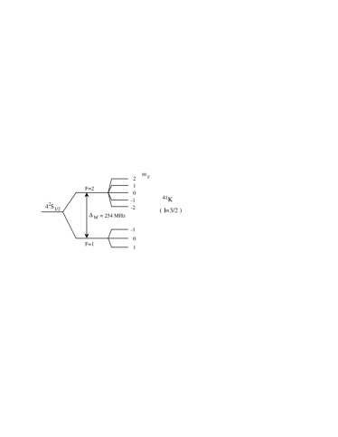
Figure 2: Schematic of the Zeeman/hyperfine structure of ⁴¹K. (For ⁴¹K atoms, $I=3/2$ and $g_{I}$=0.215.) The total angular momentum $F=I+J$ and its projection $M_{F}$ are good quantum numbers at $B=0$, and can also be used to unambiguously label the atomic levels when $B\neq 0$.

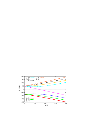
Figure 3: (Color online) Energies of the Zeeman-split ⁴¹K atomic levels as a function of magnetic field. The levels are labeled by their $(F,M_{F})$ quantum numbers when $B=0$.

III.1 Single Atom Electron Spin Matrix Elements

Alkali atoms are one-electron atoms in the sense that they have one comparatively weakly bound $s$-electron and a closed-shell electron core. Excitations of the closed-shell electron core occur at a much higher energy scale than the probes that are considered here. The atomic levels are eigenstates of the Hamiltonian of an atom (with nuclear spin $I$) interacting with an electron (spin $s=\frac{1}{2}$)

$${\mathbf{H}}^{(1)}\ =\ {\frac{\mathbf{p}^{2}}{2m}}\ +\ \mathbf{V}_{a-e}\ =\ \sum\ H^{(1)}_{k,ij}\ {\mathbf{a}}^{\dagger}_{ki}{\mathbf{a}}_{kj}\>,$$ (34)

where $\mathbf{p}^{2}/(2m)$ is the kinetic energy, $\mathbf{V}_{a-e}$ is the atom-electron potential

$$\mathbf{V}_{a-e}\ =\ A\ \vec{s}\cdot\vec{i}\ +\ \vec{B}\cdot\Bigl{(}2\mu_{e}\vec{s}-g_{I}\mu_{n}\vec{i}\Bigr{)}\>,$$ (35)

with $\mu_{e}=g_{e}\mu_{B}/2$, with $g_{e}$ = 2.0023, and $\mu_{n}=\mu_{B}/1836$. Here, $A$ denotes the strength of the hyperfine interaction, and the hyperfine splitting is $\Delta_{\rm{hf}}=(I+\frac{1}{2})A$.

The atom-level wave functions involve both nuclear and electron degrees of freedom. In the representation of nuclear and electron spins the single-particle state are

$$|i\rangle=|I_{i}M_{i}\rangle\ |s_{i}m_{i}\rangle\>,$$ (36)

with $s_{i}=1/2$. The matrix elements of the one-body Hamiltonian are

$$\langle\psi_{i}|H^{(1)}|\psi_{j}\rangle\ =\ \delta_{M_{i}M_{j}}\delta_{m_{i}m_{j}}\$$ (37)

$$\times\Bigl{[}\varepsilon(k)\ +\ \frac{A}{2}\ M_{j}\,(-)^{j}\ +\ \bigl{(}\mu_{e}\,(-)^{j}-g_{I}\mu_{n}\,M_{j}\bigr{)}\ B\Bigr{]}$$

$$\ +\ \frac{A}{2}\ \delta_{M_{i},M_{j}-1}\ \delta_{m_{i}\uparrow}\delta_{m_{j}\downarrow}\ \Bigl{[}I(I+1)-M_{j}(M_{j}-1)\Bigr{]}^{1/2}$$

$$\ +\ \frac{A}{2}\ \delta_{M_{i},M_{j}+1}\ \delta_{m_{i}\downarrow}\delta_{m_{j}\uparrow}\ \Bigl{[}I(I+1)-M_{j}(M_{j}+1)\Bigr{]}^{1/2}\>.$$

Here we denote by $j=1$ the Dirac electron spinor $|\downarrow\rangle$, and by $j=2$ the spinor $|\uparrow\rangle$.

The one-body Hamiltonian is diagonalized to obtain the atom-level states, $|\phi_{i}\rangle$

$$|\phi_{i}\rangle\ =\ \sum_{k}\ \alpha_{ik}\ |\psi_{k}\rangle\>.$$ (38)

We calculate the electron spin matrix elements

$$\langle\phi_{i}| \mathbf{\hat{n}}\cdot\sigma|\phi_{j}\rangle\ =\ \sum_{kl}\ \alpha_{ik}\ \alpha_{jl}\$$ (39)

$$\times\ \Bigl{[}\sin\theta\ \langle\psi_{k}|(\sigma_{+}+\ \sigma_{-})|\psi_{l}\rangle\ +\ \cos\theta\ \langle\psi_{k}|\sigma_{0}|\psi_{l}\rangle\Bigr{]}\>,$$

where $\mathbf{\hat{n}}=(\sin\theta,0,\cos\theta)$.

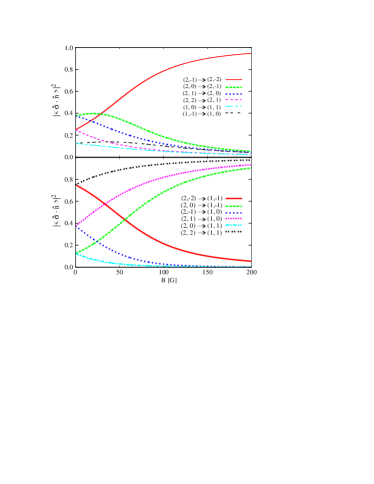
Figure 4: (Color online) Squared electron spin matrix elements for the case of transverse magnetic fields ($\theta=90^{\circ}$). The selection rule in this case is $\Delta M_{F}=\pm 1$. The top panel depicts the case of $\Delta F=0$. Because the nuclear moment of ⁴¹K is very small, the following pairs of transitions are nearly degenerate in energy (frequency): $(2,0)\rightarrow(2,-1)$ and $(1,-1)\rightarrow(1,0)$; $(2,1)\rightarrow(2,0)$ and $(1,0)\rightarrow(1,1)$. The bottom panel shows transitions for which $\Delta F=\pm 1$. The following pairs of transitions are nearly degenerate in energy (frequency): $(2,1)\rightarrow(1,0)$ and $(2,0)\rightarrow(1,1)$; $(2,0)\rightarrow(1,-1)$ and $(2,-1)\rightarrow(1,0)$.

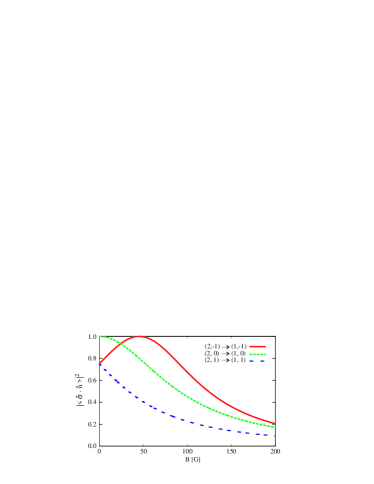
Figure 5: (Color online) Squared electron spin matrix elements in ⁴¹K for the case of longitudinal magnetic fields ($\theta=0^{\circ}$). The selection rule in this case is $\Delta M_{F}=0$.

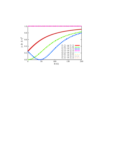
Figure 6: (Color online) Squared electron spin matrix elements in ⁴¹K for the self-excitation transitions (longitudinal magnetic fields, $\theta=0^{\circ}$). These transitions all appear at zero frequency. The self-excitation amplitudes of levels $(1,1)$ and $(2,1)$ are equal, as are the amplitudes for levels $(1,0)$ and $(2,0)$, and also for $(1,-1)$ and $(2,-1)$, respectively. The self-excitation amplitudes of $(2,-2)$ and $(2,2)$ are both equal to $1$.

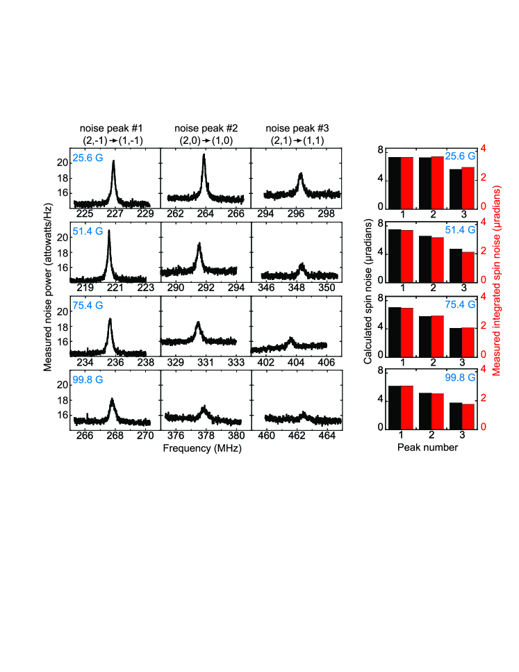
Figure 7: (Color online) The experimentally-measured noise power spectrum from a gas of ⁴¹K atoms, for longitudinal magnetic fields $B_{L}$ ($\theta=0^{\circ}$). Here, the measured noise power density (aW/Hz) is proportional to the square of Faraday rotation noise density (which has units of radians/Hz^1/2). The three allowed spin noise resonances ((2,-1)$\rightarrow$(1,-1), (2,0)$\rightarrow$(1,0), and (2,1)$\rightarrow$(1,1)) are measured at $B_{L}$ = 25.6, 51.4, 75.4, and 99.8 Gauss. Electronic detector and amplifier noise is not subtracted from this data. At the right, histograms compare the theoretically calculated spin noise (black bars) with the measured integrated spin noise (red bars), in units of Faraday rotation (microradians). The relative measured spin noise agrees well with calculation at all $B_{L}$. There is an overall (absolute) discrepancy of approximately a factor of two between theory and experiment.

For ⁴¹K atoms the nuclear spin is $I=\frac{3}{2}$, and the hyperfine splitting is $\Delta_{\rm{hf}}=2A$. The schematic of the Zeeman/hyperfine spectrum for ⁴¹K is shown in Fig. 2. The atom levels are obtained by diagonalizing the one-body Hamiltonian $H^{(1)}$, and the atom-level energies are plotted in Fig. 3 as a function of applied magnetic field $B$. At low magnetic fields where the Zeeman energies are smaller than or comparable to the hyperfine interaction, the electron and nuclear spins are entangled and no projection of electron spin is a good quantum number. At strong magnetic fields where the Zeeman splitting is much larger than the hyperfine splitting, the electron spin projection in the direction of the magnetic field becomes a good quantum number.

For transverse magnetic fields ($\theta=90^{\circ}$), the angular momentum selection rule is $\Delta M_{F}=\pm 1$, and the magnetic field dependence of the transition amplitudes is shown in Fig. 4. At low magnetic fields, there is strength for all of the $\Delta M_{F}=\pm 1$ transitions, but at high magnetic field there is strength only for those transitions corresponding to a change in the electron spin projection in the direction of the magnetic field. For longitudinal magnetic fields ($\theta=0^{\circ}$), the angular momentum selection rule is $\Delta M_{F}=0$, and the $B$ dependence of the corresponding transition amplitudes is illustrated in Fig. 5. In Fig. 6, we show the $B$ dependence of the self-transition amplitudes, present when $\theta=0^{\circ}$. At low magnetic fields, there is strength for all of the $\Delta M_{F}=0$ transitions, but at high magnetic field there is strength only for the zero frequency self transitions. The zero frequency self-transitions are hard to measure experimentally due to environmental noise sources, but they are necessary for completing the sum rule Eq. (32).

III.2 Spin correlation function

In second-quantization notation the electron-spin correlation function is

$$\langle\sigma_{z}({\bf{r}},t)\sigma_{z}(0,0)\rangle=\sum_{ijmn} \langle i|\mathbf{\hat{n}}\cdot\sigma|j\rangle\langle m|\mathbf{\hat{n}}\cdot\sigma|n\rangle$$ (40)

$$\times\ \langle e^{\mathrm{i}{\mathbf{H}}t}{\mathbf{a}}^{\dagger}_{i}{\mathbf{a}}_{j}e^{-\mathrm{i}{\mathbf{H}}t}{\mathbf{a}}^{\dagger}_{m}{\mathbf{a}}_{n}\rangle\>,$$

where $\langle O\rangle$ denotes a thermal average of the operator $O$. For a non-interacting system of atoms, ${\mathbf{H}}={\mathbf{H}}^{(1)}$, and the electron-spin correlation function becomes

$$S(\omega)=\frac{1}{\rho_{0}}\sum_{ij} \ |\langle i|\mathbf{\hat{n}}\cdot\sigma|j\rangle|^{2}\ \delta(\omega-\delta_{ij})$$ (41)

$$\times\int\frac{\mathrm{d}^{3}k}{(2\pi)^{3}}\ \rho_{k,i}\,(1-\rho_{k,j})\ \>,$$

where $\delta_{ij}$ denotes the transition energy between atomic levels $i$ and $j$ (i.e. $\delta_{ij}=E_{j}-E_{i}$), and we have introduced the density matrix $\rho_{k,i}=\langle{\mathbf{a}}^{\dagger}_{\mathbf{k}i}{\mathbf{a}}_{\mathbf{k}i}\rangle$, describing the occupation of level $i$, corresponding to momentum $k$. In the classical (high-temperature) limit, the occupation numbers are given by the Boltzmann distribution function. The product of two occupations, $\rho_{k,i}\,\rho_{k,j}$, can be neglected when compared to $\rho_{k,i}$ for a Boltzmann gas. In the high temperature limit all hyperfine/Zeeman states are equally populated and $S^{i\rightarrow j}(\omega)$ is given by

$$S^{i\rightarrow j}(\omega)=\frac{1}{N\rho_{0}}\,\delta(\omega-\delta_{ij})\>,$$ (42)

where $N$ is the number of levels in the hyperfine spectrum of the alkali atom. The $\delta$-functions can be broadened by, for example, finite spin lifetime effects or the time it takes the atoms to traverse across the laser beam.

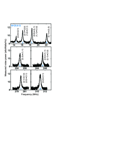
Figure 8: (Color online) The experimentally-measured noise power spectrum in a gas of ⁴¹K atoms, at a transverse magnetic field of $B_{T}$=25.6 G ($\theta=90^{\circ}$). There are twelve allowed inter- and intra-hyperfine spin noise resonances. Four pairs of resonances are nearly degenerate in frequency, giving eight resolvable spin noise peaks in the data (peaks are labeled 1-8 as shown). Background electronic noise from the detectors and amplifiers has been subtracted.

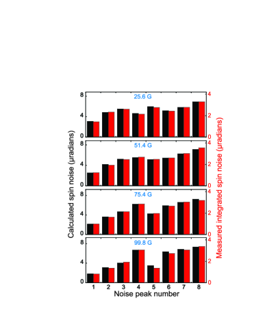
Figure 9: (Color online) Histograms comparing the calculated spin noise (black bars) with the measured integrated spin noise (red bars) for all eight resolved noise resonances in transverse magnetic fields $B_{T}$ ($\theta=90^{\circ}$), in units of Faraday rotation (microradians). Peaks are labeled in Figure 8. The relative measured spin noise agrees well with calculation for all values of $B_{T}$ (25.6, 51.4, 75.4, and 99.8 Gauss). There is an overall (absolute) discrepancy of approximately a factor of two between theory and experiment.

IV Experimental results

In this section we compare the results of our theoretical model with experimental data. We use a gas of the isotope ⁴¹K primarily because ⁴¹K has a very small hyperfine splitting (254 MHz), permitting easy access to the “high magnetic field regime” where the characteristic Zeeman energies approach and exceed the hyperfine energy. Moreover, spontaneous noise resonances in ⁴¹K occur at relatively low frequencies ($<$500 MHz), where photodetectors are generally more sensitive. We use a 1 cm long glass vapor cell containing isotopically-enriched ⁴¹K metal. The cell is typically heated to 184 ^∘C, giving a particle density of 7.3 $\times$10¹³/cm³ in the vapor. The 4 mW probe laser beam, derived from a continuous-wave Ti:Sapphire laser, is typically detuned by 100 GHz from the D1 transition (770 nm) of ⁴¹K, and Faraday rotation fluctuations on the transmitted probe laser beam are detected by fast balanced photodiodes (New Focus model 1607, which has 650 MHz bandwidth and 350 V/W gain). The resulting noise power spectrum is detected by a 500 MHz spectrum analyzer (Agilent model 4395). The detectors and amplifiers typically contribute a frequency-dependent noise density between 4-7 $\times 10^{-18}$ Watts/Hz (4-7 aW/Hz). Using 4 mW of probe laser power, photon shot noise contributes an additional 8-9 aW/Hz of measured noise. This measured value of photon shot noise varies somewhat with frequency because the gain and sensitivity of the detector/spectrum analyzer combination is not uniform across the entire 0-500 MHz range (in particular, it falls at the highest frequencies). All values of measured spin noise from the ⁴¹K atoms include this frequency-dependent correction.

Figure 7 shows the measured noise power spectrum from ⁴¹K atoms for the case of longitudinal magnetic fields ($\theta=0^{\circ}$). These raw data are plotted in units of power spectral density (aW/Hz) as measured by the spectrum analyzer. In these experiments, spin fluctuations lead to Faraday rotation fluctuations, which directly generate voltage fluctuations at the output of the photodiode bridge. Figure 7 shows the power spectrum of these voltage fluctuations (proportional to voltage squared). As such, these raw data convey the square of the spin noise (or Faraday rotation) spectral density (which itself is expressible in units of radians/Hz^1/2). The integrated power within the first noise peak of Figure 7 ((2,-1)$\rightarrow$(1,-1) at 25.6 G) is 2.0 pW, which corresponds to 10 $\mu$V of integrated voltage noise (all instruments have 50 ohm impedance). Given the 350 V/W detector sensitivity and the total optical power in the probe beam (4 mW), the integrated Faraday rotation noise for this particular spin noise resonance is 3.57 $\mu$rad.

Three spontaneous noise resonances are observable in this configuration: (2,-1)$\rightarrow$(1,-1), (2,0)$\rightarrow$(1,0), and (2,1)$\rightarrow$(1,1). Raw data for all three spin noise peaks are shown, at four different values of applied field (25.6, 51.4, 75.4, and 99.8 Gauss). On the right-hand side of the Figure, the theoretically calculated spin noise of each resonance (black bars) is compared with the integrated spin noise under each of the three measured peaks (red bars). Values of spin noise are expressed in units of Faraday rotation (microradians). In addition to the electron spin matrix elements, the calculated values take into account the overall prefactor which depends on laser detuning, power, beam size, and atom density, per Eq. (29). At any given field, the relative noise contained within the three peaks agrees very well with calculation. The absolute calculated results are approximately a factor of 2 larger than the measured results (see the scales on the histograms). As the magnetic field increases beyond 50 G and the calculated spin noise in each of the three peaks decreases (as anticipated in Fig. 5), the measured spin noise (red bars) also decreases, continuing to show good agreement with theory as the high-field regime is approached.

For transverse magnetic fields ($\theta=90^{\circ}$), twelve inter- and intra-hyperfine spin noise resonances are allowed. For brevity, Figure 8 shows the actual measured data only for the case of $B_{T}$=25.6 G. At $B_{T}$=25.6 G, eight distinct spin noise peaks are observed (because the nuclear moment of ⁴¹K is very small, four pairs of allowed noise resonances are nearly degenerate in frequency and cannot be individually resolved – see the labeling of the peaks in Fig. 8). Figure 9 shows calculated spin noise (black bars) and experimentally measured integrated spin noise for each of the eight resolved noise resonances, at $B_{T}$=25.6, 51.4, 75.4, and 99.8 Gauss (peak numbers are labeled in Figure 8). Again, the relative spin noise contained within these peaks agrees very well with theoretical prediction, but the theoretical results are approximately a factor of 2 larger than the experimental results in absolute magnitude. As the magnetic field is increased from the low to the high-field limit, the relative spin noise that is measured by experiment changes in accord with the calculations shown in Figure 4.

V Summary and conclusions

In summary, we have derived a general expression for the electron spin noise power spectrum in alkali gases as measured by Faraday rotation. We have shown that the noise power spectrum is determined by an electron spin-spin correlation function. A detailed and quantitative comparison study of the calculated spin noise was performed using experiments in a classical gas of ⁴¹K atoms, and we report good agreement between theory and experiment in both longitudinal and transverse applied magnetic fields, from low fields up to the high-field regime where Zeeman energies are comparable with hyperfine energies. The theoretical results presented here apply to both classical gases at high temperature as well as ultracold quantum gases. Because the integrated strength of the lines gives information about the occupation of the atomic levels (while the line-shapes depend on the properties of the condensed atomic state) future spin noise spectroscopy measurements may play an important role for the study of the effective interaction in ultracold atom gases.

- (1) R. Kubo, Rep. Prog. Phys. 29, 255 (1966).
- (2) E. B. Aleksandrov and V. S. Zapassky, Zh. Eksp. Teor. Fiz. 81, 132 (1981).
- (3) T. Sleator, E. L. Hahn, C. Hilbert, and J. Clarke, Phys. Rev. Lett. 55, 1742 (1985).
- (4) D. D. Awschalom, D. P. DiVincenzo, and J. F. Smyth, Science 258, 414 (1992).
- (5) M. B. Weissman, Rev. Mod. Phys. 65, 829 (1993).
- (6) J. L. Sorensen, J. Hald, and E. S. Polzik, Phys. Rev. Lett. 80, 3487 (1998).
- (7) A. Kuzmich et al., Phys. Rev. A 60, 2346 (1999).
- (8) N. Smith and P. Arnett, Appl. Phys. Lett. 78, 1448 (2001).
- (9) T. Mitsui, Phys. Rev. Lett. 84, 5292 (2000).
- (10) T. Ito, N. Shimomura, and T. Yabuzaki, J. Phys. Soc. Japan 72, 962 (2003).
- (11) S.A. Crooker, D.G. Rickel, A.V. Balatsky, and D.L. Smith, Nature (London) 431, 49 (2004).
- (12) M. Oestreich, M. Römer, R. J. Haug, and D. Hägele, Phys. Rev. Lett. 95, 216603 (2005).
- (13) For an extreme case, see H. J. Mamin, R. Budakian, B. W. Chui, and D. Rugar, Phys. Rev. Lett. 91, 207604 (2003); D. Rugar, R. Budakian, H. J. Mamin, and B. W. Chui, Nature (London) 430, 329 (2004).
- (14) W. Happer and B. S. Mathur, Phys. Rev. Lett. 18, 577 (1967).
- (15) A. Corney, Atomic and Laser Spectroscopy (Clarendon Press, Oxford, 1977).
- (16) B. Mihaila, S. A. Crooker, K. B. Blagoev, D. G. Rickel, P. B. Littlewood and D. L. Smith, cond-mat/0601011.
- (17) M. H. Anderson, J. R. Ensher, M. R. Matthews, C. E. Wieman, and E. A. Cornell, Science 269, 198 (1995).
- (18) K. B. Davis, et al., Phys. Rev. Lett. 75, 3969 (1995).
- (19) C. C. Bradley, C. A. Sackett, J. J. Tollett, and R. G. Hulet, Phys. Rev. Lett. 75, 1687 (1995).
- (20) B. DeMarco and D. S. Jin, Science 285, 1703 (1999).