Exciton Mediated One Phonon Resonant Raman Scattering from One-Dimensional Systems

Abstract

We use the Kramers-Heisenberg approach to derive a general expression for the resonant Raman scattering cross section from a one-dimensional (1D) system explicitly accounting for excitonic effects. The result should prove useful for analyzing the Raman resonance excitation profile lineshapes for a variety of 1D systems including carbon nanotubes and semiconductor quantum wires. We apply this formalism to a simple 1D model system to illustrate the similarities and differences between the free electron and correlated electron-hole theories.

I Introduction

Raman scattering is a standard optical spectroscopy technique used to characterize the excitation spectrum of a material system. If the exciting or scattered light frequency is nearly commensurate with an electronic transition of the material, the scattered Raman signal intensity is greatly enhanced Cardona and Güntherodt (1982). In semiconductors or insulators, resonant Raman scattering not only serves as a probe of a structure’s vibrational modes, but also can provide valuable information about the nature of a material’s electronic structure.

For three-dimensional (3D) bulk semiconductors Cantarero et al. (1989), two-dimensional (2D) quantum wells Zhu et al. (1989); Vina et al. (1996), zero-dimensional (0D) self-assembled quantum dots Menéndez-Proupin et al. (1999) and semiconductor microcrystallites Chamberlain et al. (1995), a Kramers-Heisenberg approach to the theory of one phonon resonant Raman scattering (1phRRS), based on either free electron-hole states (FEH) or Wannier excitonic states have been well developed. But, to our knowledge, a theory of 1phRRS incorporating excitonic effects has not been developed for a quantum confined one-dimensional (1D) system. Here we construct an expression for the resonant Raman scattering cross-section from a 1D system incorporating Wannier excitons as the intermediate electronic states. Specifically, we derive a general expression that is useful for analyzing the Raman spectra of a variety of 1D systems.

There are currently two approaches to achieving quantum confinement that results in a 1D system. One approach, in the spirit of quantum wells and quantum dots, involves introducing a potential discontinuity to confine the material’s electronic quasiparticles along the direction of discontinuity. A second approach, exemplified by single wall carbon nanotubes (SWNTs), is geometric confinement where a periodic boundary condition is used to provide single-valued solutions. For example, by rolling a graphene sheet to form a continuous tube, the allowable states of the system must exhibit phase continuity as we traverse a complete cycle around the tube in the azimuthal direction.

SWNTs are of particular interest since there has been decisive theoretical Ando (1997); Perebeinos et al. (2004); Kane and Mele (2004) and experimental Wang et al. (2005); Maultzsch et al. (2005) evidence that excitonic states dominate the optical properties of these systems. In studying SWNT, 1phRRS is a standard optical technique utilized to locate electronic resonances in SWNTs and to determine the diameter of the tube under study. With the ability to perform tunable 1phRRS on a single SWNT and map out the full Raman scattering resonant excitation profile (REP) Yin et al. , a theory of 1phRRS that explicitly accounts for the excitonic intermediate states of the scattering process is necessary.

The organization of this paper is as follows. In Section II, we develop a general expression for the 1phRRS cross-section of a 1D system. First, we solve a 1D Schrödinger equation for the Wannier exciton wavefunctions and energy eigenvalues. We use the wavefunctions to construct the appropriate interaction Hamiltonians necessary to describe the Raman scattering process. In Section III, for the particular case of a two-subband model, we illustrate the influence of excitonic states on the 1phRRS cross-section. Finally, in Section IV we present a summary of the work and a comparison between 1phRRS and 1D absorption.

II Theory of One Phonon Raman Scattering from a One-Dimensional System

The general 1D material system we consider is illustrated in Fig. 1.

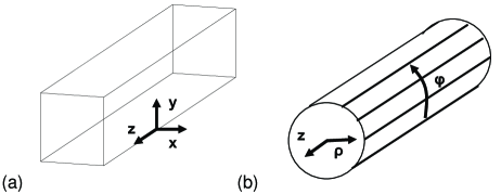
Figure 1: Two typical one-dimensional quantum confined systems. (a) illustrates a rectangular quantum wire and (b) a cylindrical tube.

We imagine the system is illuminated by a laser beam of fixed frequency ${\omega_{l}}$, propagation direction $\vec{q}_{l}$ and polarization $\vec{e}_{l}$. The inelastically scattered radiation propagates in direction $\vec{q}_{s}$ with fixed polarization $\vec{e}_{s}$ and is collected so that its spectral content, $\omega_{s}$, may be analyzed with a spectrometer. Without loss of generality, we focus on the Stokes scattering process. Microscopically, an incident pump photon interacts with the unexcited system, creates an electronic excitation that scatters a phonon before relaxing radiatively back to its ground state by emitting a photon. We use Fermi’s golden rule to determine the Stokes differential Raman scattering cross-section integrated over all scattered photon wavenumbers. The resulting expression is Cardona and Güntherodt (1982)

$$\frac{d\sigma_{RRS}}{d\Omega}=\frac{\omega_{s}^{3}n_{s}^{3}n_{l}V^{2}_{crystal}}{\omega_{l}c^{4}(2\pi\hbar)^{2}}\cdot|W_{i\rightarrow f}(\omega_{l},\vec{e_{l}};\omega_{s}=\omega_{l}-\Omega_{p},\vec{e_{s}})|^{2}$$ (1)

where $c$ is the speed of light in free space, $n_{i}$ is the refractive index of the material evaluated at frequency $\omega_{i}$, $V_{crystal}$ is the volume of the material system and $|W_{i\rightarrow f}|^{2}$ is the transition probability from initial system state $i$, with a single pump photon, to a final state $f$, with a single scattered photon and a single phonon. Using third order time-dependent perturbation theory, the transition matrix element $|W_{i\rightarrow f}|^{2}$ from initial state $|initial>$ to final state $|final>$ can be expressed as

$$W_{i\rightarrow f}=\sum_{a,b}\frac{<final|\hat{H}_{int}|b><b|\hat{H}_{int}|a><a|\hat{H}_{int}|initial>}{(E_{initial}-E_{b}-i\Gamma_{b})(E_{initial}-E_{a}-i\Gamma_{a})}$$ (2)

where the sum over $a$ and $b$ is over all permissible intermediate states, $E_{j}$ is the energy associated with state $j$, $\hat{H}_{int}$ is the appropriate interaction Hamiltonian (to be defined below), $\Gamma_{j}$ is a phenomenological broadening parameter that incorporates the finite lifetime of intermediate states $j=a,b$ and $i$ is the imaginary unit $\sqrt{-1}$. To evaluate Eq. (2), we will use the language of second quantization and specify the states in the occupation number representation. In this notation, a general state is a direct product of state vectors where each component state vector belongs to the sector of the Hilbert space appropriate for the excitation; $|state>=|electronic>\otimes|phonon>\otimes|photon>$. We label each state by the number of quanta in a given mode. For example, $|photon>=|0_{\vec{q}_{s},\vec{e}_{s}},1_{\vec{q}_{l},\vec{e}_{l}}>$ when there is a single photon in the laser mode and there is no scattered photon. The role of the interaction Hamiltonian, $\hat{H}_{int}$, in this perturbative treatment is to allow quanta to be exchanged between the different sectors of Hilbert space. $\hat{H}_{int}$ can be expressed as $\hat{H}_{int}=\hat{H}^{(X-R)}_{int}+\hat{H}^{(X-L)}_{int}$ where we have decomposed the interaction Hamiltonian into a piece $\hat{H}^{(X-R)}_{int}$ that couples the excitons with the photons (R=radiation) and a piece $\hat{H}^{(X-L)}_{int}$ that couples the excitons with the phonons (L=lattice). Here it is important to note that the intermediate electronic excitations will be treated as correlated electron-holes, or excitons, and not as free electrons and holes.

Upon substitution of $\hat{H}_{int}$ into Eq. (2) and requiring energy conservation, we find there are six possible pathways or probability amplitudes that can contribute to $|W_{i\rightarrow f}|^{2}$. In the following we focus only on the contribution of the resonant path because the other five pathways make a comparatively negligble contribution to the cross-section. The contribution of the resonant pathway can be expressed as

$$W_{i\rightarrow f}=\sum_{a,b}\frac{<final|\hat{H}_{int}^{(X-R)}|b><b|\hat{H}_{int}^{(X-L)}|a><a|\hat{H}_{int}^{(X-R)}|initial>}{(\hbar\omega_{l}-\hbar\Omega_{p}-E_{b}-i\Gamma_{b})(\hbar\omega_{l}-E_{a}-i\Gamma_{a})}.$$ (3)

To proceed further we define the exciton-radiation interaction Hamiltonian $\hat{H}^{(X-R)}_{int}$, assuming the minimal coupling interaction and retaining only the term linear in the electromagnetic vector potential, written in second quantized notation as Cantarero et al. (1989)

$$\hat{H}_{int}^{(X-R)}=\sum_{\begin{subarray}{c}X,\vec{K}_{cm}\\ \\ \vec{q},\vec{e}\end{subarray}}T_{cv}^{X}(\vec{K}_{cm})\hat{D}^{\dagger}_{X,\vec{K}_{cm}}\hat{a}_{\vec{q},\vec{e}}+T_{cv}^{*X}(\vec{K}_{cm})\hat{D}_{X,\vec{K}_{cm}}\hat{a}^{\dagger}_{\vec{q},\vec{e}}$$ (4)

where the exciton-radiation coupling constant can be expressed as

$$T_{cv}^{X}(\vec{K}_{cm}=\vec{k}_{e}-\vec{k}_{h})=\frac{e}{m_{o}}\sqrt{\frac{2\pi\hbar}{V_{crystal}\omega n^{2}}}<X_{2}|e^{i\vec{q}\cdot\vec{r}}\vec{e}\cdot\vec{\hat{p}}|X_{1}>$$ (5)

and $\hat{D}_{X,K_{cm}},\hat{D}^{\dagger}_{X,K_{cm}}$ ($(\hat{a}_{\vec{q},\vec{e}},\hat{a}^{\dagger}_{\vec{q},\vec{e}})$) are the annhilation and creation operators for excitons (photons), $e$ is the electronic charge, $m_{o}$ is the bare electron mass, $\vec{\hat{p}}$ is the electronic momentum operator and $|X_{j}>$ are exciton wavefunctions.

Similarly, focusing only on phonon creation processes, the exciton-lattice interaction Hamiltonian for coupling with a single phonon branch can be expressed as

$$\hat{H}_{int}^{(X-L)}=\sum_{\begin{subarray}{c}X_{1},\vec{K}_{cm,1}\\ \\ X_{2},\vec{K}_{cm,2}\\ \\ \vec{Q}\end{subarray}}S_{X_{1}}^{X_{2}}(\vec{Q})\hat{D}^{\dagger}_{X_{2},\vec{K}_{cm,2}}\hat{D}_{X_{1},\vec{K}_{cm,1}}\hat{b}^{\dagger}_{\vec{Q}}$$ (6)

where the exciton-lattice coupling constant is

$$S_{X_{1}}^{X_{2}}(\vec{Q})=<X_{2}|C(\vec{r}_{e})e^{-i\vec{Q}\cdot\vec{r}_{e}}-C(\vec{r}_{h})e^{-i\vec{Q}\cdot\vec{r}_{h}}|X_{1}>$$ (7)

and $\vec{Q}$ is the phonon momentum, $\hat{b}^{\dagger}_{\vec{Q}}$ is the phonon creation operator, and $C(\vec{r_{j}})$ depend on the details of the exact exciton-phonon interaction. Two common examples of exciton-phonon interactions are deformation potential coupling and Frölich coupling Stroscio and Dutta (2005). To determine the explicit form of both $\hat{H}_{int}^{(X-R)}$ and $\hat{H}_{int}^{(X-L)}$ we need expressions for the 1D exciton wavefunctions $|X_{j}>$ so that we can evaluate the appropriate coupling constants.

To obtain expressions for the exciton wavefunctions, we will use both the effective mass approximation (EMA) and the envelope function approximation (EFA)Haug and Koch (2001). These approximations reduce the complicated problem of solving the Schrödinger equation, for the two-particle Bloch wavefunction to solving the following modified Schrödinger equation Ogawa and Takagahara (1991)

$$\Biggl{[}-\frac{\hbar^{2}}{2m_{e}^{*}}\nabla^{2}_{e}-\frac{\hbar^{2}}{2m_{h}^{*}}\nabla^{2}_{h}+V(\vec{r}_{e})+V(\vec{r}_{h})+V_{3}(\vec{r}_{e},\vec{r}_{h})\Biggr{]}\Phi(\vec{r}_{e},\vec{r}_{h})=E\Phi(\vec{r}_{e},\vec{r}_{h})$$ (8)

for the envelope function $\Phi(\vec{r}_{e},\vec{r}_{h})$ of the exciton where the influence of the periodic crystal potential has been incorporated into the problem by replacing the bare electron (hole) mass with the effective electron (hole) mass $m_{e}^{*}$ ($m_{h}^{*}$) and by multiplying the solution of Eq. (8) by the Bloch functions of the conduction $u_{c}(\vec{r})$ and valence band $u_{v}(\vec{r})$ (for the unconfined system) to calculate the approximate two-particle Bloch wavefunction $\Psi(\vec{r}_{e},\vec{r}_{h})\approxeq\Phi(\vec{r}_{e},\vec{r}_{h})u_{c}(\vec{r}_{e})u_{v}(\vec{r}_{h})$. In Eq. (8), $V(\vec{r}_{j})$ is the potential that confines particle $j$ and $V_{3}(\vec{r}_{e},\vec{r}_{h})$ is the 3D Coulomb potential. Assuming we have solved the problem of electron and hole confinement, we can expand the exciton envelope function in the basis of the confined electron and hole wavefunctions as

$$\Phi(\vec{r}_{e},\vec{r}_{h})=\sum_{\begin{subarray}{c}(l_{e}^{a},l_{e}^{b},l_{h}^{a},l_{h}^{b})\\ integers\end{subarray}}e^{iK_{cm}Z_{cm}}\phi_{x}^{(l_{e}^{a},l_{e}^{b},l_{h}^{a},l_{h}^{b})}(z_{r}=z_{e}-z_{h})f^{l_{e}^{a}}(x_{e}^{a})f^{l_{e}^{b}}(x_{e}^{b})f^{l_{h}^{a}}(x_{h}^{a})f^{l_{h}^{b}}(x_{h}^{b})$$ (9)

where $x^{j}_{i}$ denotes the $j^{th}$ coordinate for particle $i$, $f^{l_{i}^{j}}$ is the complete and orthonormal confined wavefunction for particle $i$ in subband labeled by $l_{i}^{j}$ confined in the $j^{th}$ coordinate direction and, anticipating a change to center of mass coordinates along the unconfined direction, $\phi_{x}^{(l_{e}^{a},l_{e}^{b},l_{h}^{a},l_{h}^{b})}(z_{r}=z_{e}-z_{h})$ is a function characterizing the relative motion of the electron and hole. In Eq. (9), we have assumed that the confining potential is along two spatial directions and unconfined motion is along a third orthogonal direction. For example, in Fig. 1(a), electronic motion is confined along the $x$ and $y$ directions while it is unconfined along the $z$ direction. If we began with a material system that was initially 2D, and then further confined along one spatial direction, we would supress all functions and coordinates in Eq. (9) labeled with $b$. Equation (9) expresses the two-particle envelope function as a superposition of confined electron and hole states, weighted by a function describing the 1D excitonic state associated with the subbands $(l_{e}^{a},l_{e}^{b},l_{h}^{a},l_{h}^{b})$. Finally, we substitute Eq. (9) into Eq. (8) and project the resulting equation over a set of confined wavefunctions with labels $(l_{e}^{a},l_{e}^{b},l_{h}^{a},l_{h}^{b})$. Here we neglect the possibility of subband coupling due to the Coulomb potential, a reasonable assumption for large subband energy spacing, and arrive at the following, effective 1D Schrödinger equation for the relative motion of the electron and hole

$$\Biggl{[}-\frac{\hbar^{2}}{2\mu}\frac{d^{2}}{d^{2}z_{r}}+V_{1-eff}^{(l_{e}^{a},l_{e}^{b},l_{h}^{a},l_{h}^{b})}(z_{r})\Biggr{]}\phi_{x}^{(l_{e}^{a},l_{e}^{b},l_{h}^{a},l_{h}^{b})}(z_{r})=E_{x}^{(l^{e}_{a},l^{e}_{b},l^{h}_{a},l^{h}_{b})}(K_{cm})\phi_{x}^{(l_{e}^{a},l_{e}^{b},l_{h}^{a},l_{h}^{b})}(z_{r})$$ (10)

where $\mu^{-1}=\frac{1}{m_{e}^{*}}+\frac{1}{m_{h}^{*}}$ is the electron and hole effective reduced mass and $E_{x}^{(l_{e}^{a},l_{e}^{b},l_{h}^{a},l_{h}^{b})}(K_{cm})$ is the exciton binding energy. $E_{x}^{(l_{e}^{a},l_{e}^{b},l_{h}^{a},l_{h}^{b})}(K_{cm})$ is expressible as $E_{x}^{(l_{e}^{a},l_{e}^{b},l_{h}^{a},l_{h}^{b})}(K_{cm})=E-E^{bare}_{gap}-E_{e}^{(l_{e}^{a},l_{e}^{b})}-E_{h}^{(l_{h}^{a},l_{h}^{b})}-\frac{\hbar^{2}K_{cm}^{2}}{2M}$ where $M=m_{e}^{*}+m_{h}^{*}$, $E_{e}^{(l_{e}^{a},l_{e}^{b})}$ ($E_{h}^{(l_{h}^{a},l_{h}^{b})}$) is the confinement energy of the electron (hole) in the $(l_{e}^{a},l_{e}^{b})$ ($(l_{h}^{a},l_{h}^{b})$) subbands, $\frac{\hbar^{2}K_{cm}^{2}}{2M}$ is the center of mass motion of the exciton and $V_{1-eff}^{(l_{e}^{a},l_{e}^{b},l_{h}^{a},l_{h}^{b})}(z_{r})$ is expressed as

$$V_{1-eff}^{(l_{e}^{a},l_{e}^{b},l_{h}^{a},l_{h}^{b})}(z_{r})=\int_{-\infty}^{\infty}dx^{a}_{e}dx_{e}^{b}dx^{a}_{h}dx^{b}_{h}|f^{l_{e}^{a}}(x_{e}^{a})|^{2}|f^{l_{e}^{b}}(x_{e}^{b})|^{2}|f^{l_{h}^{a}}(x_{h}^{a})|^{2}|f^{l_{h}^{b}}(x_{h}^{b})|^{2}V_{3}(\vec{r}_{e},\vec{r}_{h}).$$ (11)

The previous equation is an average of the full 3D Coulomb potential weighted by the probabilities of finding the electron and hole along the confined directions. The averaging results in a potential that depends on only the electron and hole coordinates along the unconfined direction. In what follows we label the exitonic states as $X=(x,K_{cm},l_{e}^{a},l_{e}^{b},l_{h}^{a},l_{h}^{b})$. The label $x$ is discrete or continuous depending on whether the exciton is bound or unbound, $K_{cm}$ is the exciton center of mass momentum and $(l_{e}^{a},l_{e}^{b},l_{h}^{a},l_{h}^{b})$ label the subbands of the electron and hole that comprise the exciton.

To simplify the following calculations, we follow Loudon Loudon (1959) and model $V_{1-eff}^{(l_{e}^{a},l_{e}^{b},l_{h}^{a},l_{h}^{b})}(z_{r})$ as

$$V_{1-eff}^{(l_{e}^{a},l_{e}^{b},l_{h}^{a},l_{h}^{b})}(z_{r})=V_{1-eff}(z_{r})=-\frac{e^{2}}{\epsilon(|z_{r}|+z_{o})}$$ (12)

where $\epsilon$ is the dielectric constant of the material and $z_{o}$ is a fit parameter. It is possible, using the confined electron and hole wavefunctions, to evaluate Eq. (11) and find a value of $z_{o}$ such that Eq. (12) is a good approximation to Eq. (11). The inclusion of $z_{o}$ in Eq. (12) removes the singularity at the origin of the 1D Coulomb potential and allows us to solve Eq. (10). The solution of Eq. (10) for the 1D excitonic relative motion wavefunction has been discussed in detail in other works and we refer the reader to these referencesOgawa and Takagahara (1991); Combescot and Guillet (2004).

Using the solution to Eq. (8), we evaluate the momentum matrix element in Eq. (5) between the exciton vacuum $|X_{1}>=|0>$ and an excited exciton state $|X_{2}>=|X>$. We find the exciton-radiation coupling is expressed as Chuang (1995)

$$T_{cv}^{X}(K_{cm})=\frac{e}{m_{o}}\sqrt{\frac{2\pi\hbar}{V_{crystal}\omega n^{2}}}\vec{e}\cdot\vec{p}_{cv}\sum_{(l_{e}^{a},l_{e}^{b},l_{h}^{a},l_{h}^{b})}Y_{l_{e}^{a}}^{l_{h}^{a}}Y_{l_{e}^{b}}^{l_{h}^{b}}\phi_{x}^{*(l_{e}^{a},l_{e}^{b},l_{h}^{a},l_{h}^{b})}(z_{r}=0)\delta_{K_{cm}=k_{e}-k_{h},q}$$ (13)

where

$$\vec{p}_{cv}=\frac{1}{V_{unit}}\int_{V_{unit}}\,d\vec{r}\,u_{c}^{*}(\vec{r})\Biggl{(}\frac{i}{\hbar}\nabla u_{v}(\vec{r})\Biggr{)}$$ (14)

is the momentum matrix element of the Bloch functions over a unit cell of volume $V_{unit}$,

$$Y_{l_{e}^{j}}^{l_{h}^{j}}=\int\,dx^{j}f^{l_{e}^{j}}(x^{j})f^{l_{h}^{j}}(x^{j})$$ (15)

is an integral calculating the overlap of the subband electron and hole wavefunctions across the domain $x^{j}$ with $j=a,b$, $\phi_{x}^{*(l_{e}^{a},l_{e}^{b},l_{h}^{a},l_{h}^{b})}(z_{r}=0)$ is the envelope function of the 1D electron-hole relative motion of the type $x$ exciton between subbands $(l_{e}^{a},l_{e}^{b},l_{h}^{a},l_{h}^{b})$ evaluated at zero electron-hole separation and $\delta_{K_{cm}=k_{e}-k_{h},q}$ is the Kronecker delta function expressing conservation of momentum along the unconfined direction. We point out that $Y_{l_{e}^{j}}^{l_{h}^{j}}$ is equal to $\delta_{l_{e}^{j},l_{h}^{j}}$ when the electron and hole experience identical confinement potentials, which we will use in Section III.

Similarly, we evaluate Eq. (7) between two excited exciton states $|X_{1}>$ and $|X_{2}>$. We find the exciton-lattice coupling constant is expressible as

$$S_{X_{1}}^{X_{2}}=\delta_{K_{cm,1},K_{cm,2}+Q}\Biggl{[}\delta_{l_{h,2},l_{h,1}}C^{l_{e,2}}_{l_{e,1}}B^{X_{2}}_{X_{1}}(\alpha_{e}Q)-\delta_{l_{e,2},l_{e,1}}C^{l_{h,2}}_{l_{h,1}}B^{X_{2}}_{X_{1}}(\alpha_{h}Q)\Biggr{]}$$ (16)

where $\alpha_{e}=\frac{m_{h}^{*}}{M}$, $\alpha_{h}=-\frac{m_{e}^{*}}{M}$, $\delta_{l_{j,2},l_{j,1}}$ implies the $j^{th}$ particle stays in its subbands after the exciton scatters from the phonon and the phonon mediated intermediate excitonic state coupling has been decomposed into a piece related to the exciton relative motion wavefunction

$$B^{X_{2}}_{X_{1}}(Q)=\int\,dz_{r}\phi_{x_{2}}^{*(l_{e,2}^{a},l_{e,2}^{b},l_{h,2}^{a},l_{h,2}^{b})}(z_{r})e^{-iQz_{r}}\phi_{x_{1}}^{(l_{e,1}^{a},l_{e,1}^{b},l_{h,1}^{a},l_{h,1}^{b})}(z_{r})$$ (17)

and a piece depending on the details of how the possibly confined phonon Stroscio and Dutta (2005) couples with the confined electron and hole

$$C^{l_{i,2}}_{l_{i,1}}=\int\,dx_{i}^{a}dx_{i}^{b}f^{*l_{i,2}^{a}}(x_{i}^{a})f^{*l_{i,2}^{b}}(x_{i}^{b})C(x_{i}^{a},x_{i}^{b})f^{l_{i,1}^{a}}(x_{i}^{a})f^{l_{i,1}^{b}}(x_{i}^{b})$$ (18)

with $i=e$ or $i=h$.

We now substitute Eq. (13) and Eq. (16) into Eq. (3) and assume the photon momentum may be neglected when compared to the electron and hole crystal momentum (the k-selection rule)

$$W_{i\rightarrow f}=\sum_{X_{1},X_{2}}M_{\begin{subarray}{c}(l^{a}_{e,2},l^{b}_{e,2},l^{a}_{h,2},l^{b}_{h,2})\\ (l^{a}_{e,1},l^{b}_{e,1},l^{a}_{h,1},l^{b}_{h,1})\end{subarray}}^{cv}\frac{\phi_{x_{2}}^{(l^{a}_{e,2},l^{b}_{e,2},l^{a}_{h,2},l^{b}_{h,2})}(0)B^{X_{2}}_{X_{1}}(Q=0)\phi_{x_{1}}^{*(l^{a}_{e,1},l^{b}_{e,1},l^{a}_{h,1},l^{b}_{h,1})}(0)}{(\hbar\omega_{l}-\hbar\Omega_{p}-E_{b}-i\Gamma_{b})(\hbar\omega_{l}-E_{a}-i\Gamma_{a})}$$ (19)

where the coupling constant is given by

$$M_{\begin{subarray}{c}(l^{a}_{e,2},l^{b}_{e,2},l^{a}_{h,2},l^{b}_{h,2})\\ (l^{a}_{e,1},l^{b}_{e,1},l^{a}_{h,1},l^{b}_{h,1})\end{subarray}}^{cv}=\frac{e^{2}(2\pi\hbar)^{2}(\vec{e}_{s}\cdot\vec{p}^{*}_{vc})(\vec{e}_{l}\cdot\vec{p}_{cv})}{m_{o}^{2}V_{crystal}\sqrt{\omega_{s}\omega_{l}}n_{s}n_{l}}Y_{l_{e,2}^{a}}^{*l_{h,2}^{a}}Y_{l_{e,2}^{b}}^{*l_{h,2}^{b}}Y_{l_{e,1}^{a}}^{l_{h,1}^{a}}Y_{l_{e,1}^{b}}^{l_{h,1}^{b}}[\delta_{l_{h,2},l_{h,1}}C^{l_{e,2}}_{l_{e,1}}-\delta_{l_{e,2},l_{e,1}}C^{l_{h,2}}_{l_{h,1}}].$$ (20)

Finally, substituting Eq. (19) and Eq. (20) into Eq. (1) we arrive at

$$\frac{d\sigma_{RRS}}{d\Omega}=\frac{e^{4}\omega_{s}^{2}n_{s}}{c^{4}m_{o}^{4}\omega_{l}^{2}n_{l}}\Biggl{|}\sum_{X_{1},X_{2}}\bar{M}_{\begin{subarray}{c}(l^{a}_{e,2},l^{b}_{e,2},l^{a}_{h,2},l^{b}_{h,2})\\ (l^{a}_{e,1},l^{b}_{e,1},l^{a}_{h,1},l^{b}_{h,1})\end{subarray}}^{cv}\frac{\phi_{x_{2}}^{(l^{a}_{e,2},l^{b}_{e,2},l^{a}_{h,2},l^{b}_{h,2})}B^{X_{2}}_{X_{1}}\phi_{x_{1}}^{*(l^{a}_{e,1},l^{b}_{e,1},l^{a}_{h,1},l^{b}_{h,1})}}{(\hbar\omega_{l}-\hbar\Omega_{p}-E_{b}-i\Gamma_{b})(\hbar\omega_{l}-E_{a}-i\Gamma_{a})}\Biggr{|}^{2}$$ (21)

where $\bar{M}$ is defined in a similar manner to Eq. (20), but the constants have been factored out and we have supressed the arguments in both $\phi_{x}^{l}$ and $B_{X_{1}}^{X_{2}}$. The double summation extends over all intermediate excitonic states.

Equation (21) is the central result of the paper and provides a general expression for calculating the scattering cross-section of resonant Raman scattering, using third-order time dependent perturbation theory, from a 1D quantum confined structure when the intermediate electronic excitations are excitonic in nature. In Eq. (21), we have factored the numerator into a part that depends on the relative motion of the 1D excitons and a part that is a function of both the electron and hole subband confined wavefunctions and the Bloch functions from which the exciton is built. The utility of this decomposition is that we can focus explicitly on how the 1D exciton influences the Raman scattering cross-section. If we are interested in a particular material system, and wish to obtain an absolute value for its Raman scattering cross-section, it would be necessary to evaluate all the system-specific matrix elements in Eq. (20). It should be noted that Eq. (21) allows for the possibility of Raman scattering between both bound and unbound intermediate excitonic states. In the next section we calculate the Raman scattering cross-section for a model 1D system with only a single conduction and valence subband for which we assume the potentials confining the electron and hole are identical for simplicity.

III Two-Subband Model

In this section, we give an explicit expression for Eq. (21) when the material system is composed of only a single conduction and valence subband ($(l_{e}^{a},l_{e}^{b},l_{h}^{a},l_{h}^{b})=(1_{e}^{a},1_{e}^{b},1_{h}^{a},1_{h}^{b})$) and the electron and hole experience identical confining potentials. Fig. 2(a) illustrates the single particle bandstructure for the system which is assumed to be known.

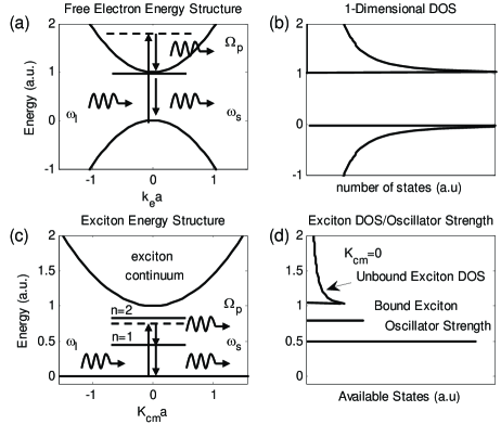
Figure 2: The (a) free electron electronic structure, (b) the free electron density of states, (c) the excitonic electronic structure and (d) the unbound excitonic $K_{cm}=0$ density of states and bound exciton oscillator strengths. In (a), the free electron energies are functions of the electron crystal momentum, whereas in (c), the excitonic energies are functions of the exciton center of mass momentum. The dispersion associated with the bound excitons has not been illustrated since in exciton mediated transtions, only $K_{cm}=0$ transitions are allowed due to conservation of momentum. In addition, in (a) and (c), an outgoing Stokes resonance is illustrated where the dashed horizontal line corresponds to a virtual electronic state and a solid horizontal line corresponds to a real electronic state. In each case, a photon of energy $\hbar\omega_{l}$ causes an electronic transition to a virtual state, followed by the electronic excitation relaxing to a real, electronic state by emitting a phonon of energy $\hbar\Omega_{p}$. Finally, the electronic system returns to its ground state by emitting a photon of energy $\hbar\omega_{s}$. This can be compared to the free electron mediated transitions where only vertical transitons are allowed, but $k_{e}$ is not constrained to be 0.

Using the single particle bandstructure and wavefunctions, we can solve Eq. (10) for the exciton energy eigenvalues, and visualize the electronic structure of our material system in Fig. 2(c). Incorporating excitonic effects has resulted in a series of bound states below the quantum confined system’s energy gap of $E_{gap}^{bare}+E_{e}^{(1_{e}^{a},1_{e}^{b})}+E_{h}^{(1_{h}^{a},1_{h}^{b})}$ in addition to the usual continuum of states above this energy gap. As discussed in Loudon Loudon (1959), the internal energy label for bound exciton states is no longer constrained to a set of postive integers, but is describable by a set of positive real numbers. Within this two-subband approximation, we can simplify Eq. (21) as follows

$$\frac{d\sigma_{RRS}}{d\Omega}(\omega_{l};\omega_{s}=\omega_{l}-\Omega_{p})=R|L_{bound}(\omega_{l};\omega_{s}=\omega_{l}-\Omega_{p})+L_{unbound}(\omega_{l};\omega_{s}=\omega_{l}-\Omega_{p})|^{2}$$ (22)

where $L_{bound}$ and $L_{unbound}$ are functions that characterize the influence that the bound and unbound excitons have on the Raman scattering cross-section and we have collected all the constants of Eq. (21) in $R$. In this two-subband model, transitions between intermediate exciton states, with different values of $x$, are forbidden by $B_{X_{1}}^{X_{2}}$ in Eq. (17) when we assume the k-selection rule and neglect the phonon momentum $Q$. For transitions between different excitonic states to be possible, there must be non-zero overlap between the two intermediate states that participate in the Raman scattering process. Overlap can arise if the excitons are derived from subbands with different effective masses and therefore have unequal Bohr radii.

Specific expressions for $L_{bound}$ and $L_{unbound}$ are

$$L_{bound}(\omega_{l};\omega_{s}=\omega_{l}-\Omega_{p})=\sum_{n}\frac{|\phi_{n}(0)|^{2}}{(\hbar\omega_{s}-E_{gap}+\frac{R^{*}}{n^{2}}-i\Gamma_{b})(\hbar\omega_{l}-E_{gap}+\frac{R^{*}}{n^{2}}-i\Gamma_{a})}$$ (23)

and

$$L_{unbound}(\omega_{l};\omega_{s}=\omega_{l}-\Omega_{p})=\int_{E_{gap}}^{E_{c}}\,dE\frac{|\phi_{E}(0)|^{2}}{\sqrt{E_{gap}-E}(\hbar\omega_{s}-E_{gap}-E-i\Gamma_{b})(\hbar\omega_{l}-E_{gap}-E-i\Gamma_{a})}$$ (24)

where $R^{*}$ is the effective exciton Rydberg, $E_{c}$ is an energy cutoff to the above integral and the summation in Eq. (23) includes only even envelope functions. In Eq. (23) (Eq. (24)), the sum over all intermediate states has been reduced to a sum (an integral) over the label associated with the internal energy of the exciton.

With Eqs. (23) and (24), we use both the bound and unbound exciton relative motion wavefunctions to evaluate the lineshape of the exciton mediated Raman scattering cross-section. In evaluating the bound and unbound wavefunctions with Eq. (10), we have freedom in how we choose $z_{o}$, the parameter introduced to make the 1D Coulomb potential finite at the origin. The closer $z_{o}$ is to zero, the greater the 1D character of the problem we are solving. Since the majority of physical systems exhibiting properties characteristic of a 1D system typically are not truly 1D, finite values of $z_{o}$ are physically reasonable. For example, in a SWNT, the tube radius provides a natural value for $z_{o}$. The procedure to correctly determine $z_{o}$ is to select $z_{o}$ such that Eq. (12) approximates Eq. (11).

Before evaluating the full lineshape function Eq. (22), we will focus on the individual contributions of the bound and unbound excitons. Fig. 3 illustrates the contributions of the first four bound excitons to the bound lineshape function Eq. (23) as a function of laser energy $\hbar\omega_{l}$. The two peak structure apparent in the 1phRRS cross-section mediated by each bound exciton is a result of an incoming and an outgoing resonance. These resonances are associated with the incoming (laser) or outgoing (scattered) photon being coincident in energy with the bound exciton internal energy. The dependence of the 1phRRS on excitation frequency is commonly referred to as a Resonance Excitation Profile (REP) and we will adhere to this terminology. In Fig. 3, all exciton REPs are normalized relative to the ground state exciton mediated transition (the top figure).

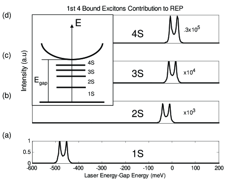
Figure 3: The (a) 1S,(b) 2S,(c) 3S and (d) 4S bound exciton REP. In all figures, $z_{o}/a_{X}=.2$, $\Gamma=5$ meV, $R^{*}=100$ meV and $\hbar\Omega_{p}=32$ meV. The double peak structure in the REP is due to both an incoming resonance, when $\hbar\omega_{l}=E_{gap}$, and an outgoing resonance, when $\hbar\omega_{s}=E_{gap}$.

To calculate each REP, we assumed a dephasing of $\Gamma_{a}=\Gamma_{b}=5$ meV, a phonon of energy $\hbar\Omega_{p}=32$ meV and we set $E_{gap}=E^{bare}_{gap}+E_{e}^{(1_{e}^{a},1_{e}^{b})}+E_{h}^{(1_{h}^{a},1_{h}^{b})}$ to be the zero of the energy scale. In addition, we chose the Rydberg $R^{*}=100$ meV. The reason for choosing this value is that it sets the ground state exciton binding energy to approximately 500 meV, a value determined in recent measurements on SWNTs Wang et al. (2005). It is clear in Fig. 3 that the ground state exciton dominates the bound exciton mediated lineshape function. The contribution to the REP from the ground state exciton is nearly 3 orders of magnitude stronger than that of the next bound excited exciton.

Next, with the same set of parameters, we compare, in absolute terms, the unbound exciton contribution to the exciton mediated REP with the contribution of the strongest bound exciton. To make this comparison we plot Eq. (23) in Fig. 4(a) and Eq. (24) in Fig. 4(b).

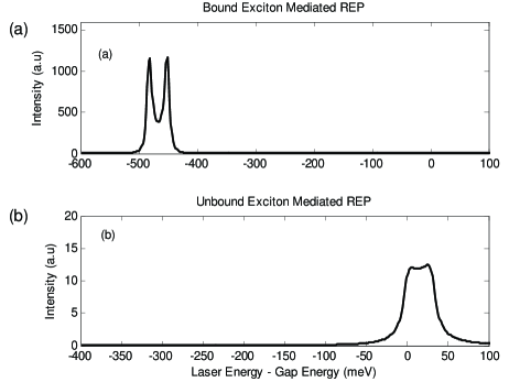
Figure 4: Comparison of the relative strength of the (a) bound exciton mediated REP with the (b) unbound exciton mediated REP. In (a) and (b), $z_{o}/a_{X}=0.2$, $\Gamma=5$ meV, $R^{*}=100$ meV and $\hbar\Omega_{p}=32$ meV.

The strength of the bound exciton mediated REP is nearly 2 orders of magnitude larger than the unbound exciton. It is clear that $|\phi_{x}(0)|^{2}$ strongly influences how efficiently a given exciton can mediate the 1phRRS process. Similar to it effect in 1D absorption Ogawa and Takagahara (1991), $|\phi_{x}(0)|^{2}$ acts to suppress the contribution of the unbound exciton to the exciton mediated REP.

With an understanding of how both the bound and unbound exciton contribute individually to the REP, we now evaluate Eq. (22) for the full exciton mediated 1phRRS REP. Since we will compare our result with the REP of the free electron-hole (FEH) theory for 1phRRS, we quote the result for the free electron-hole theory Raman scattering cross-section Cardona and Güntherodt (1982)

$$\frac{d\sigma^{FEH}_{RRS}}{d\Omega}(\omega_{l};\omega_{s}=\omega_{l}-\Omega_{p})=\frac{e^{4}\omega_{s}^{2}n_{s}}{c^{4}m_{o}^{4}\omega_{l}^{2}n_{l}}\frac{\pi^{2}}{\hbar^{2}\Omega^{2}_{p}}\Biggl{|}\frac{1}{\sqrt{(\hbar\omega_{l}-\hbar\Omega_{p}-E_{gap}}}-\frac{1}{\sqrt{i\Gamma_{b})(\hbar\omega_{l}-E_{gap}-i\Gamma_{a})}}\Biggr{|}^{2}.$$ (25)

Figure 5 compares Eq. (22) with Eq. (25).

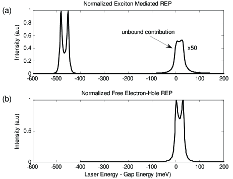
Figure 5: Comparison of the normalized (a) exciton mediated REP with the (b) Free electron-hole mediated REP. In (a) and (b), $\Gamma=5$ meV, $R^{*}=100$ meV and $\hbar\Omega_{p}=32$ meV. In addition, in (a), $z_{o}/a_{X}=0.2$. Notice in (a) the small contribution of the unbound excitons.

It is immediately clear from Fig. 5(a) that the energies at which the system strongly Raman scatters incident laser light is shifted to the lowest bound exciton. Nonetheless, there is a small feature at the band gap associated with light Raman scattered using unbound exciton intermediate states. In addition, the incoming and outgoing peaks are more pronounced in the exciton mediated REP as compared to the FEH REP. Practically, though, such small qualitative differences in the REP are likely to be experimentally undetectable. Besides the gross shift in energy, the REPs generated by both theories appear quite similar.

At this point it is important to recall that, in solving Eq. (10), we set the ratio of the potential cutoff to the exciton Bohr radius, ${z_{o}}/{a_{X}}$, equal to 0.2. If we further reduce $z_{o}\rightarrow 0$, the lowest bound exciton will only become more dominant in mediating the REP. With this in mind, we finally investigate the dependence of the exciton mediated REP on $z_{o}/a_{X}$. In particular, we now set $z_{o}/a_{X}=1$. Physically, the Bohr radius of the exciton is equal to the cutoff of the 1D Coulomb potential and, as $z_{o}$ increases, the system becomes less 1D. In Fig. 6, we keep all input parameters from Fig. 5 fixed except $z_{o}/a_{X}$ is changed to 1.

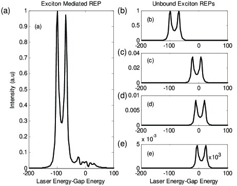
Figure 6: The (a) exciton mediated REP and in (b)-(e), the REPs of the first four bound excitons. In (a)-(e), $z_{o}/a_{X}=1$, $\Gamma=5$ meV, $R^{*}=100$ meV and $\hbar\Omega_{p}=32$ meV. Notice the structure present at the location of the free electron bandgap.

First, the higher excited bound excitons (Fig. 6(b)-6(e)) make larger individual contributions to the exciton mediated REPs. When we examine the full exciton mediated REP, we find there is some structure in the vicinity of the the free electron band gap. We can understand this structure as follows. As the binding energy of the ground state exciton decreases, the relative strength of the scattering process mediated by the lowest bound exciton (as compared to the other bound excitons) also decreases. In addition, the REPs that we have attributed to the various bound excitons begin to overlap. In fact, as the overlap increases, the REP at a fixed $\hbar\omega_{l}$ is the result of a quantum interference between all excitonic pathways that can contribute effectively to the scattering process.

IV Conclusion

We have developed a general theory for calculating the exciton mediated one phonon resonant Raman scattering cross-section for 1D quantum confined systems (Eq. (21)). In studying a model two-subband system, we found the exciton was strongly bound when $z_{o}$ is small compared to the exciton Bohr radius $a_{X}$. In this limit of small $z_{o}$, the ground state exciton dominates the 1phRRS REP. The contribution to the REP from unbound excitons with energies in the range of the single particle gap energy is quenched. The quenching is similar in origin to the suppression of the exciton mediated absorption coefficient at energies above a 1D material system’s bare energy gap; the ground state exciton carries all the spectral weight in the transition Ogawa and Takagahara (1991). As the Coulomb potential cutoff $z_{o}$ is increased, the ground state becomes more weakly bound, and we found that both the higher excited bound and unbound excitons begins to contribute to the 1phRRS REP. As $z_{o}$ approaches the excitonic Bohr radius $a_{X}$, the REP, at a fixed laser frequency, is the result of a quantum interference between all contributing intermediate excitonic pathways. The interferences lead to a complicated structure at the single particle energy gap. The shape of the 1phRRS REP provides a qualitative indicator of how much spectral weight the ground state exciton carries in mediating the 1phRRS process.

The sensitivity of the 1phRRS REP to changes in the potential cutoff is a physically important effect. Although the cutoff is introduced to make tractable the analytic solution of the Schrödinger equation with the 1D Coulomb potential tractable, the majority of physically realizable quantum confined 1D systems are more accurately described as quasi-1D. For example, both semiconductor quantum wires and SWNTs have finite spatial extent in the directions perpendicular to the direction of unconfined motion. The finite extent in these spatial directions lends itself naturally to the introduction of a cutoff in the Coulomb potential.

In applying our results to specific material systems, such as semiconductor quantum wires or SWNTs, it is necessary to evaluate matrix elements specific to each material system. Though not discussed in this work, we also observe that if we allow for the possibility of more than two subbands, it becomes possible to observe true double resonances in the 1phRRS REP. Specifically, the phonon could scatter the intermediate exciton between two real, bound states. We leave such investigations to future work.

References

• Cardona and Güntherodt (1982) M. Cardona and G. Güntherodt, eds., Light Scattering in Solids II (Springer ,Heidelberg, 1982), vol. 50 of Topics in Applied Physics, chap. 2, p. 19.
• Cantarero et al. (1989) A. Cantarero, C. Trallero-Giner, and M. Cardona, Phys. Rev. B 39, 8388 (1989).
• Zhu et al. (1989) B. Zhu, K. Huang, and H. Tang, Phys. Rev. B 40, 6299 (1989).
• Vina et al. (1996) L. Vina, J. M. Calleja, A. Cros, A. Cantarero, T. Berendschot, J. A. Perenboom, and K. Ploog, Phys. Rev. B 53, 3975 (1996).
• Menéndez-Proupin et al. (1999) E. Menéndez-Proupin, C. Trallero-Giner, and S. E. Ulloa, Phys. Rev. B 60, 16747 (1999).
• Chamberlain et al. (1995) M. P. Chamberlain, C. Trallero-Giner, and M. Cardona, Phys. Rev. B 51, 1680 (1995).
• Ando (1997) T. Ando, J. Phys. Soc. Jpn. 66, 1066 (1997).
• Perebeinos et al. (2004) V. Perebeinos, J. Tersoff, and P. Avouris, Phys. Rev Lett. 92, 257402 (2004).
• Kane and Mele (2004) C. L. Kane and E. J. Mele, Phys. Rev. Lett. 93, 197402 (2004).
• Wang et al. (2005) F. Wang, G. Dukovic, L. E. Brus, and T. F. Heinz, Science 308, 838 (2005).
• Maultzsch et al. (2005) J. Maultzsch, R. Pomraenke, S. Reich, E. Chang, D. Prezzi, A. Ruini, E. Molinari, M. S. Strano, C. Thomsen, and C. Lienau, Phys. Rev. B 72, 241402(R) (2005).
• (12) Y. Yin, S. Cronin, A. Walsh, A. Stolyarov, M. Tinkham, A. N. Vamivakas, W. Basca, M. S. Ünlü, B. B. Goldberg, and A. K. Swan, to be published.
• Stroscio and Dutta (2005) M. A. Stroscio and M. Dutta, Phonons in Nanostructures (Cambridge University Press, 2005).
• Haug and Koch (2001) H. Haug and S. W. Koch, Quantum Theory of the Optical and Electronic Properties of Semiconductors (World Scientific, Singapore, 2001), third edition ed.
• Ogawa and Takagahara (1991) T. Ogawa and T. Takagahara, Phys. Rev. B 44, 8138 (1991).
• Loudon (1959) R. Loudon, Am. J. Phys. 27, 649 (1959).
• Combescot and Guillet (2004) M. Combescot and T. Guillet, Eur Phys. J. B 37, 413 (2004).
• Chuang (1995) S. L. Chuang, Physics of Optoelectronic Devices (Wiley, New York, 1995).