Quasiparticle states of the Hubbard model near the Fermi level

Abstract

The spectra of the $t$-$U$ and $t$-$t^{\prime}$-$U$ Hubbard models are investigated in the one-loop approximation for different values of the electron filling. It is shown that the four-band structure which is inherent in the case of half-filling and low temperatures persists also for some excess or deficiency of electrons. Besides, with some departure from half-filling an additional narrow band of quasiparticle states arises near the Fermi level. The dispersion of the band, its bandwidth and the variation with filling are close to those of the spin-polaron band of the $t$-$J$ model. For moderate doping spectral intensities in the new band and in one of the inner bands of the four-band structure decrease as the Fermi level is approached which leads to the appearance of a pseudogap in the spectrum.

I Introduction

In the last two decades the discovery of high-$T_{c}$ superconductors, heavy-fermion compounds and organic conductors has revived interest in strongly correlated electron systems. One of the simplest and still realistic models in this field is the one-band Hubbard model two-dimensional version of which has been extensively studied in connection with the cuprate perovskite superconductors. Along with Monte-Carlo simulations, Moreo ; Grober different cluster methods, Maier ; Aichhorn ; Tremblay the operator projection technique, Mancini the generating functional approach, Izyumov05 various versions of the diagram technique Zaitsev ; Izyumov ; Ovchinnikov ; Vladimir ; Metzner ; Pairault are used for the investigation of the model. In a system in which the Coulomb interaction dominates, it is reasonable to treat this interaction exactly and the kinetic energy in the framework of a perturbation theory.

In the diagram technique proposed in Refs. Vladimir, ; Metzner, ; Pairault, the power expansion is expressed in terms of site cumulants of electron creation and annihilation operators. From the expansion the Larkin equation for the electron Green’s function can be derived. Vladimir ; Pairault ; Sherman06 The equation can be solved in the one-loop approximation. However, the obtained solution has a flaw – a negative spectral weight in two narrow frequency regions. Pairault This flaw can be remedied by an interpolation using results for regular regions. Sherman06 The obtained spectral function Sherman06 was shown to be in agreement with results of Monte-Carlo simulations Grober at half-filling and for moderate temperatures when the magnetic correlation length is comparable with the intersite distance. In particular, it was shown that in agreement with results of Monte-Carlo and cluster methods Moreo ; Grober ; Maier ; Aichhorn ; Tremblay the diagram technique is able to describe the four-band structure of the spectrum at half-filling.

In the present paper the same method is used for the investigation of the energy spectrum at a departure from half-filling. It is shown that in this case the above-mentioned four bands persist and additionally a new band arises in some vicinity of the Fermi level. By its properties – the dispersion, bandwidth and the variation with filling – the band resembles the spin-polaron band of the $t$-$J$ model. Dagotto For moderate doping the spectral intensities in the new band and in one of the inner bands of the four-band structure decrease as the Fermi level is approached. This produces a pseudogap near the Fermi level. For the hole-doped case, $\bar{n}<1$, the magnitude of the pseudogap observed in photoemission decreases with increasing the hole doping $1-\bar{n}$, while for the electron-doped case, $\bar{n}>1$, this magnitude increases with increasing the electron doping $\bar{n}-1$. Here $\bar{n}$ is the electron concentration. Together with the $t$-$U$ Hubbard model the $t$-$t^{\prime}$-$U$ model is also considered for the ratio $t^{\prime}/t=-0.3$ of the next-nearest and nearest neighbor hopping constants. Korshunov As for the case of half-filling the calculated spectral functions and dispersions appear to be similar to those obtained by Monte-Carlo and cluster methods, provided that doping or temperature are high enough to ensure a short magnetic correlation length.

Main formulas used in the calculations are given in the following section (the detailed derivation of these formulas can be found in Ref. Sherman06, ). The discussion of the obtained results and their comparison with results of other methods are carried out in Sec. III and IV for the $t$-$U$ and $t$-$t^{\prime}$-$U$ models, respectively. Concluding remarks are presented in Sec. V.

II Main formulas

The Hamiltonian of the Hubbard model reads

$$H=\sum_{\bf nm\sigma}t_{\bf nm}a^{\dagger}_{\bf n\sigma}a_{\bf m\sigma}+\frac{U}{2}\sum_{\bf n\sigma}n_{\bf n\sigma}n_{\bf n,-\sigma},$$ (1)

where $t_{\bf nm}$ is the hopping constants, the operator $a^{\dagger}_{\bf n\sigma}$ creates an electron on the site n of the two-dimensional square lattice with the spin projection $\sigma=\pm 1$, $U$ is the on-site Coulomb repulsion and the electron number operator $n_{\bf n\sigma}=a^{\dagger}_{\bf n\sigma}a_{\bf n\sigma}$.

The diagram technique proposed in Refs. Vladimir, and Metzner, is used in the present work for calculating Green’s function

$$G({\bf n^{\prime}\tau^{\prime},n\tau})=\langle{\cal T}\bar{a}_{\bf n^{\prime}\sigma}(\tau^{\prime})a_{\bf n\sigma}(\tau)\rangle,$$ (2)

where the angular brackets denote the statistical averaging with the Hamiltonian ${\cal H}=H-\mu\sum_{\bf n\sigma}n_{\bf n\sigma}$, $\mu$ is the chemical potential, ${\cal T}$ is the time-ordering operator which arranges other operators from right to left in ascending order of times $\tau$, $a_{\bf n\sigma}(\tau)=\exp({\cal H}\tau)a_{\bf n\sigma}\exp(-{\cal H}\tau)$, and $\bar{a}_{\bf n\sigma}(\tau)=\exp({\cal H}\tau)a^{\dagger}_{\bf n\sigma}\exp(-{\cal H}\tau)$. With the use of the diagram technique the following Larkin equation is derived Vladimir ; Pairault ; Sherman06 for the Fourier transform of function (2):

$$G({\bf k},i\omega_{l})=\frac{K({\bf k},i\omega_{l})}{1-t_{\bf k}K({\bf k},i\omega_{l})},$$ (3)

where $t_{\bf k}=\sum_{\bf n}e^{-i{\bf k(n-m)}}t_{\bf nm}$, $\omega_{l}=(2l+1)\pi T$ is the Matsubara frequency with the temperature $T$ and an integer $l$, $K({\bf k},i\omega_{l})$ is the sum of all irreducible diagrams – the diagrams which cannot be divided into two parts by cutting a hopping line. Such diagrams which appear in the first four orders of the perturbation expansion in powers of $t_{\bf nm}$ are shown in Fig. 1 with their signs and prefactors.

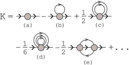
Figure 1: Irreducible diagrams of the first four orders of the expansion in powers of $t_{\bf nm}$.

Here circles are cumulants Kubo of electron operators. In diagrams, the order of a cumulant is determined by a number of incoming or outgoing hopping lines (directed lines in Fig. 1). Cumulants of the first and second orders which will be used below read

$$K_{1}(\tau^{\prime}\sigma^{\prime},\tau\sigma)=\langle{\cal T}\bar{a}_{\sigma}(\tau^{\prime})a_{\sigma}(\tau)\rangle_{0}\delta_{\sigma\sigma^{\prime}},$$

$$K_{2}(\tau^{\prime}\sigma,\tau\sigma,\tau^{\prime}_{1}\sigma_{1},\tau_{1}\sigma_{1})=$$

$$\quad\langle{\cal T}\bar{a}_{\sigma}(\tau^{\prime})a_{\sigma}(\tau)\bar{a}_{\sigma_{1}}(\tau^{\prime}_{1})a_{\sigma_{1}}(\tau_{1})\rangle_{0}$$

$$\quad-K_{1}(\tau^{\prime}\sigma,\tau\sigma)K_{1}(\tau^{\prime}_{1}\sigma_{1},\tau_{1}\sigma_{1})$$

$$\quad+K_{1}(\tau^{\prime}\sigma,\tau_{1}\sigma_{1})K_{1}(\tau^{\prime}_{1}\sigma_{1},\tau\sigma),$$

where the subscript “0” near the angular bracket indicates that the averaging and time dependencies of the operators are determined by the site Hamiltonian $H_{\bf n}=\sum_{\sigma}[(U/2)n_{\bf n\sigma}n_{\bf n,-\sigma}-\mu n_{\bf n\sigma}]$. All operators in the cumulants belong to the same lattice site. Due to the translational symmetry the cumulants do not depend on the site index which is therefore omitted in the above equations.

Partial summation is implied in the diagrams in Fig. 1 – the irreducible diagrams are included in the hopping lines which therefore correspond to the expression

$$\Theta({\bf k},i\omega_{l})=\frac{t_{\bf k}}{1-t_{\bf k}K({\bf k},i\omega_{l})}=t_{\bf k}+t_{\bf k}^{2}G({\bf k},i\omega_{l}).$$ (4)

In the one-loop approximation used below, the total collection of irreducible diagrams $K({\bf k},i\omega_{l})$ is substituted by the sum of the two diagrams (a) and (b) in Fig. 1. Thus,

$$K(i\omega_{l}) = K_{1}(i\omega_{l})-T\sum_{l_{1}\sigma_{1}}K_{2}(i\omega_{l}\sigma,i\omega_{l_{1}}\sigma_{1},i\omega_{l_{1}}\sigma_{1})$$ (5)

$$\times\frac{1}{N}\sum_{\bf k}t^{2}_{\bf k}G({\bf k},i\omega_{l_{1}}),$$

where $K_{1}(i\omega_{l})$ and $K_{2}(i\omega_{l}\sigma,i\omega_{l_{1}}\sigma_{1},i\omega_{l_{1}}\sigma_{1})$ are the Fourier transforms of the cumulants of the first and second orders, respectively, $N$ is the number of sites and I set $\sum_{\bf k}t_{\bf k}=0$. Notice that in this approximation $K$ does not depend on momentum. The cumulants read Sherman06

$$K_{1}(i\omega_{l})=\frac{1}{Z_{0}}\left(\frac{e^{-\beta E_{1}}+e^{-\beta E_{0}}}{i\omega_{l}-E_{10}}+\frac{e^{-\beta E_{2}}+e^{-\beta E_{1}}}{i\omega_{l}-E_{21}}\right),$$

$$\sum_{\sigma_{1}}K_{2}(i\omega_{l}\sigma,i\omega_{l_{1}}\sigma_{1},\omega_{l_{1}}\sigma_{1})=-Z_{0}^{-1}U\bigl{\{}e^{-\beta E_{0}}g_{01}(i\omega_{l})$$

$$\quad\times g_{01}(i\omega_{l_{1}})g_{02}(i\omega_{l}+i\omega_{l_{1}})\bigl{[}g_{01}(i\omega_{l})+g_{01}(i\omega_{l_{1}})\bigr{]}$$

$$\quad+e^{-\beta E_{2}}g_{12}(i\omega_{l})g_{12}(i\omega_{l_{1}})g_{02}(i\omega_{l}+i\omega_{l_{1}})\bigl{[}g_{12}(i\omega_{l})$$

$$\quad+g_{12}(i\omega_{l_{1}})\bigr{]}+e^{-\beta E_{1}}\bigl{[}g_{01}(i\omega_{l})g_{12}(i\omega_{l})\bigl{(}g_{01}(i\omega_{l_{1}})$$

(6)

$$\quad-g_{12}(i\omega_{l_{1}})\bigr{)}^{2}+g_{01}(i\omega_{l_{1}})g_{12}(i\omega_{l_{1}})\bigl{(}g_{01}^{2}(i\omega_{l})$$

$$\quad+g_{12}^{2}(i\omega_{l})\bigr{)}\bigr{]}\bigr{\}}-Z_{0}^{-2}U^{2}\beta\delta_{ll_{1}}\bigl{(}e^{-\beta(E_{0}+E_{2})}$$

$$\quad+2e^{-\beta(E_{0}+E_{1})}+3e^{-2\beta E_{1}}+2e^{-\beta(E_{1}+E_{2})}\bigr{)}g_{01}^{2}(i\omega_{l})$$

$$\quad\times g_{12}^{2}(i\omega_{l})+Z_{0}^{-2}U^{2}\beta\bigl{(}2e^{-\beta(E_{0}+E_{2})}+e^{-\beta(E_{0}+E_{1})}$$

$$\quad+e^{-\beta(E_{1}+E_{2})}\bigr{)}g_{01}(i\omega_{l})g_{12}(i\omega_{l})g_{01}(i\omega_{l_{1}})g_{12}(i\omega_{l_{1}}),$$

where $\beta=T^{-1}$, $E_{0}=0$, $E_{1}=-\mu$, and $E_{2}=U-2\mu$ are the eigenenergies of the site Hamiltonian $H_{\bf n}$, $E_{ij}=E_{i}-E_{j}$, $Z_{0}=e^{-\beta E_{0}}+2e^{-\beta E_{1}}+e^{-\beta E_{2}}$ is the site partition function, $g_{ij}(i\omega_{l})=(i\omega_{l}+E_{ij})^{-1}$.

Equations (6) can be significantly simplified for the case of principal interest $U\gg T$. In this case if $\mu$ satisfies the condition

$$\lambda<\mu<U-\lambda,$$ (7)

where $\lambda\gg T$, the exponent $e^{-\beta E_{1}}$ is much larger than $e^{-\beta E_{0}}$ and $e^{-\beta E_{2}}$. By passing to real frequencies one can ascertain that terms in $\sum_{\sigma_{1}}K_{2}$ with the two latter multipliers contain the same peculiarities as terms with $e^{-\beta E_{1}}$. Therefore terms with $e^{-\beta E_{0}}$ and $e^{-\beta E_{2}}$ can be omitted and Eq. (6) is simplified to

$$K_{1}(i\omega_{l})=\frac{i\omega_{l}+\mu-U/2}{(i\omega_{l}+\mu)(i\omega_{l}+\mu-U)},$$ (8)

$$\sum_{\sigma_{1}}K_{2}(i\omega_{l}\sigma,i\omega_{l_{1}}\sigma_{1},i\omega_{l_{1}}\sigma_{1})$$

$$\quad=-\frac{1}{2}Ug_{01}(i\omega_{l})g_{12}(i\omega_{l})\Bigl{[}g_{01}^{2}(i\omega_{l_{1}})+g_{12}^{2}(i\omega_{l_{1}})\Bigr{]}$$

$$\quad\quad-\frac{1}{2}Ug_{01}(i\omega_{l_{1}})g_{12}(i\omega_{l_{1}})\Bigl{[}g_{01}(i\omega_{l})-g_{12}(i\omega_{l})\Bigr{]}^{2}$$

$$\quad\quad-\frac{3}{4}U^{2}\beta\delta_{ll_{1}}g_{01}^{2}(i\omega_{l})g_{12}^{2}(i\omega_{l}).$$ (9)

Further simplification can be achieved by using the Hubbard-I approximation Hubbard for the Green’s function $G({\bf k},i\omega_{l_{1}})$ on the right-hand side of Eq. (5). The respective expression is derived from Eq. (3) if the total irreducible part $K({\bf k},i\omega_{l})$ is approximated by the first cumulant $K_{1}(i\omega_{l})$ [the diagram (a) in Fig. 1] from Eqs. (6) or (8). Izyumov ; Vladimir ; Pairault This gives

$$G({\bf k},i\omega_{l}) = \frac{1}{2}\left(1+\frac{t_{\bf k}}{\sqrt{U^{2}+t_{\bf k}^{2}}}\right)\frac{1}{i\omega_{l}-\varepsilon_{1,\bf k}}$$

$$+\frac{1}{2}\left(1-\frac{t_{\bf k}}{\sqrt{U^{2}+t_{\bf k}^{2}}}\right)\frac{1}{i\omega_{l}-\varepsilon_{2,\bf k}},$$

$$\varepsilon_{1,\bf k} = \frac{1}{2}\left(U+t_{\bf k}+\sqrt{U^{2}+t_{\bf k}^{2}}\right)-\mu,$$

$$\varepsilon_{2,\bf k} = \frac{1}{2}\left(U+t_{\bf k}-\sqrt{U^{2}+t_{\bf k}^{2}}\right)-\mu.$$

After carrying out the summation over $l_{1}$ in Eq. (5) with the use of Eqs. (8)–(LABEL:HubbardI) it is convenient to turn to real frequencies by substituting $i\omega_{l}$ with $z=\omega+i\eta$ where $\eta$ is a small positive constant which affords an artificial broadening.

III The $t$-$U$ model

At first let us consider the $t$-$U$ model in which only the nearest neighbor hopping constant $t$ is nonzero and $t_{\bf k}=2t[\cos(k_{x})+\cos(k_{y})]$. Here the intersite distance is taken as the unit of length. Due to the electron-hole symmetry in this case the consideration can be restricted to the range of the chemical potentials $\mu\leq U/2$.

Figure 2: The imaginary part of $K(\omega)$ calculated using Eqs. (5) and (8)–(LABEL:HubbardI) for a 100$\times$100 lattice, $t=-U/8$ and $T=0.001U$ (the dashed lines). (a) $\mu=0.5U$, $\eta=0.01U$. (b) $\mu=0.1U$, $\eta=0.02U$. The solid lines show the corrected ${\rm Im}K(\omega)$ (see text).

Figure 2 demonstrates ${\rm Im}K(\omega)$ calculated with the use of Eqs. (5) and (8)–(LABEL:HubbardI). The change to real frequencies converts the Matsubara function (2) into the retarded Green’s function. Abrikosov It is an analytic function in the upper half-plane which requires that ${\rm Im}K(\omega)$ be negative. As seen from Fig. 2, this condition is violated at $\omega_{d}=-\mu$ and $U-\mu$. The problem is connected with divergencies at these frequencies introduced by functions $g_{01}(\omega)$ and $g_{12}(\omega)$ in the above formulas. As can be seen from the procedure of calculating the cumulants, these functions and divergencies with sign-changing residues will appear in all orders of the perturbation theory. It can be expected that in the entire series the divergencies compensate each other and the resulting ${\rm Im}K(\omega)$ is negative everywhere. However, in the considered subset of terms such compensation does not occur. Nevertheless, as seen from Fig. 2, at frequencies neighboring to $\omega_{d}$ the irreducible part is regular and, if the used subset of diagrams is expected to give a correct estimate of the entire series for these frequencies, the values of ${\rm Im}K(\omega)$ near $\omega_{d}$ can be reconstructed using an interpolation and its values in the regular region. Sherman06 Examples of such interpolation are given in Fig. 2. The function $K(z)$ has to be analytic in the upper half-plane also and therefore its real part can be calculated from its imaginary part using the Kramers-Kronig relations. I used this way with the interpolated ${\rm Im}K(\omega)$ to avoid the influence of the divergencies on ${\rm Re}K(\omega)$. However, the application of the interpolation overrates somewhat values of $|{\rm Im}K(\omega)|$ which leads to the overestimation of the tails in the real part. To correct this defect the interpolated $K(\omega)$ is scaled so that in the far tails its real part coincides with the values obtained from equation (5).

Figure 3: The spectral function $A({\bf k}\omega)$ of the $t$-$U$ model calculated for momenta along the symmetry lines of the square Brillouin zone in a 40$\times$40 lattice for $t=-U/8$, $T=0.001U$, $\eta=0.02U$, $\mu=0.2U$ (a), and $\mu=0.1U$ (b).

As seen from Fig. 2a, at half-filling, $\mu=U/2$, ${\rm Im}K(\omega)$ has two broad minima. With decreasing the chemical potential from this value the minima shift with respect to the Fermi level without a noticeable change of their shapes until the Fermi level enters the left minimum which for $t=-U/8$ occurs at $\mu\approx 0.17U$. As this takes place, two new sharp minima arise near frequencies $-\mu$ and $U-\mu$ on the background of the above-mentioned broad minima (see Fig. 2b). The appearance of the broad features in Fig. 2 is connected with the third term on the right-hand side of Eq. (9), while the sharp minima are related to the second term in this formula. Its contribution to $K(\omega)$, Eq. (5), grows rapidly when the Fermi level enters the broad minimum.

The spectral function

$$A({\bf k}\omega) = -\frac{1}{\pi}{\rm Im}G({\bf k}\omega)$$ (11)

$$= -\frac{1}{\pi}\frac{{\rm Im}K(\omega)}{[1-t_{\bf k}{\rm Re}K(\omega)]^{2}+[t_{\bf k}{\rm Im}K(\omega)]^{2}}$$

obtained from such calculated irreducible part for momenta along the symmetry lines of the square Brillouin zone is shown in Fig. 3. The shapes of the spectral function in Fig. 3a are nearly the same as at half-filling Sherman06 – as in the case of $K(\omega)$, with decreasing $\mu$ from $U/2$ to $0.17U$ these curves shift with respect to the Fermi level without perceptible changes in their shape. In agreement with results of Monte-Carlo simulations Moreo ; Grober and cluster methods Maier ; Aichhorn ; Tremblay four bands can be distinguished in these spectra. For parameters of Fig. 3a these bands are located near the frequencies $-4|t|$, 0, $4|t|$, and $9|t|$. For the major part of the Brillouin zone maxima forming the bands arise at frequencies which satisfy the equation $1-t_{\bf k}{\rm Re}K(\omega)=0$ and fall into the region of a small damping $|{\rm Im}K(\omega)|$ [see Eq. (11)]. As seen from Fig. 2, such regions of small damping are located between and on the outside of the two broad minima in ${\rm Im}K(\omega)$. This is the reason of the existence of the four well separated bands – two of them are located between the minima of ${\rm Im}K(\omega)$, while two others are on the outside of these minima. Broader maxima of $A({\bf k}\omega)$ for momenta near the boundary of the magnetic Brillouin zone are of different nature – since $t_{\bf k}$ is small for such momenta, the resonant denominator in Eq. (11) does not vanish and the broad maxima in the spectral functions reproduce the maxima of $-{\rm Im}K(\omega)$ in the numerator of this formula.

More substantial changes in $A({\bf k}\omega)$ occur for $\mu\lesssim 0.17U$. As seen from Fig. 3b, the four-band structure persists also in this case. In addition to this there appear sharp dispersive features near $\omega=-\mu$ and $U-\mu$, the latter feature being substantially weaker in the case of hole doping, $\mu<U/2$. It is clear that these changes in the spectral function are connected with the changes in ${\rm Im}K(\omega)$ shown in Fig. 2. For the hole-doping case the peaks near $-\mu$ are located in the nearest vicinity of the Fermi level. For the parameters of Fig. 3b neither these peaks nor the peaks forming the lower inner band cross the Fermi level – their intensities decrease as it is approached. As a consequence a pseudogap arises in the spectrum near the Fermi level. Recently spectra with analogous pseudogaps were also obtained by cluster methods. Maier ; Tremblay ; Senechal ; Kyung ; Macridin In these works such spectral peculiarities were identified with the pseudogap observed in the photoemission of cuprates. Damascelli

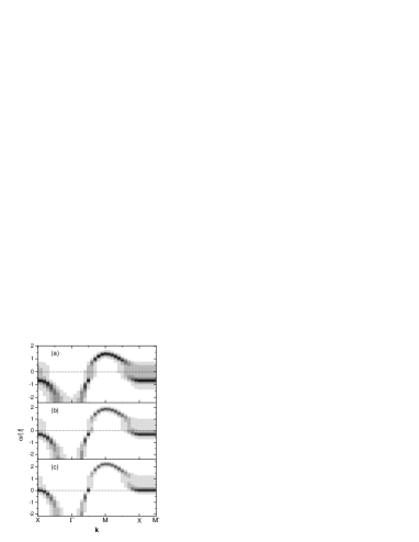
Figure 4: The dispersion of maxima of the spectral function in the $t$-$U$ model on a 20$\times$20 lattice for $t=-U/8$, $T=0.001U$, $\eta=0.02U$, $\mu=0.1U$ (a), $0.05U$ (b), and $0.01U$ (c). Here darker areas correspond to larger intensities. The points X, $\Gamma$, M, and M’ correspond to the momenta $(\pi,0)$, $(0,0)$, $(\pi,\pi)$, and $(\pi/2,\pi/2)$, respectively.

Figure 4 demonstrates the dispersion of maxima of the spectral function near the Fermi level for three values of the chemical potential. These maxima form the lover inner band above the Fermi level and the new band arising at $\mu\approx 0.17U$ below and at the Fermi level. At this value of the chemical potential the width of the new band is approximately equal to $|t|=2J$ where $J=4t^{2}/U$ is the superexchange constant of the effective Heisenberg model which describes magnetic excitations in the limit $U\gg|t|$. Izyumov ; Dagotto The bandwidth decreases with reduction in the electron concentration. The maximum energies of the band are located near the boundary of the magnetic Brillouin zone. The dispersion is much larger in the direction $(\pi/2,\pi/2)-(0,0)$ than along the boundary of the magnetic Brillouin zone $(\pi,0)-(0,\pi)$. These properties of the band resembles those of the spin-polaron band of the $t$-$J$ model. This latter band is also located near the Fermi level, has the similar dispersion and the bandwidth, which decreases with decreasing $\bar{n}$. Dagotto ; Sherman94 As seen from Fig. 4, with decreasing $\mu$ and $\bar{n}$ the Fermi level shifts to the lower edge of the pseudogap and enters the new band at $\mu\approx 0.07U$. In the photoemission which probes the part of the spectral function occupied by electrons this change in the energy spectrum will look like the decrease with the subsequent disappearance of the pseudogap with decreasing the electron concentration. Such behavior of the pseudogap is indeed observed in hole-doped cuprates. Damascelli Notice that in the case of electron doping the pseudogap observed in photoemission will grow with $\bar{n}$ until the Fermi level enters the new band (see Fig. 7).

The intensity plot of the spectral function at the Fermi level is shown in Fig. 5. The plot was obtained by averaging the spectral function in the frequency range $[-0.01U,+0.01U]$. The dark area which corresponds to the maximum intensity can be interpreted as the Fermi surface in the region of the chemical potential $0.12U\lesssim\mu\lesssim 0.25U$ where the lower inner band crosses the Fermi level (see Fig. 3a), and for $\mu\lesssim 0.07U$ where the crossing occurs with the new band (see Figs. 4b and c). For $\mu$ in the intermediate region maxima of both bands lose their intensities as the Fermi level is approached (see Figs. 3b and 4a). However, also in this case the intensity plot is similar to that shown in Fig. 5.

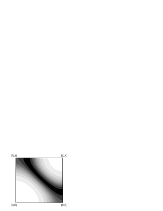
Figure 5: The intensity plot of the spectral function at the Fermi level in the first quadrant of the Brillouin zone. The darker areas correspond to larger intensities. The $t$-$U$ model on a 40$\times$40 lattice with the parameters $t=-U/8$, $T=0.001U$, $\eta=0.02U$, and $\mu=0.05U$.

With decreasing $\mu$ and $\bar{n}$ the Fermi surface shrinks to the center of the Brillouin zone and near $\mu=0.01U$ changes its shape from a diamond centered at $(\pi,\pi)$ to that centered at $(0,0)$. In contrast to the results of the cluster methods Senechal ; Kyung ; Macridin in the used approximation the variation of the intensity along the Fermi surface is small both in the $t$-$U$ and $t$-$t^{\prime}$-$U$ models.

Figure 6: The spectral function $A({\bf k}\omega)$ of the $t$-$t^{\prime}$-$U$ model calculated for momenta along the symmetry lines of the square Brillouin zone in a 40$\times$40 lattice for $t=-U/8$, $t^{\prime}/t=-0.3$, $T=0.001U$, $\eta=0.02U$, $\mu=0.1U$ (a), and $\mu=0.9U$ (b).

For the case of half-filling comparison with the data of Monte-Carlo simulations Grober shows that the spectra of the one-loop approximation are closer to the results obtained at $T=0.33|t|$ than to those derived for $T=0.1|t|$. Sherman06 The value $T=0.33|t|$ is close to the superexchange constant $J$ for $t=-U/8$. For such temperatures, the correlation length of the short-range antiferromagnetic order is comparable to the intersite distance. Shimahara Thus, it can be concluded that the one-loop approximation is more appropriate for short correlation lengths. This conclusion is also corroborated by the shapes of the spectral function in Fig. 3a which, as mentioned, are close to those at half-filling. In this figure there are no indications that the unit cell is doubled which manifests itself in a replication of some parts of the quasiparticle dispersion with the period $(\pi,\pi)$. Such a doubling is inherent in the antiferromagnetic order with a correlation length which is much larger than the lattice spacing. This limitation of the one-loop approximation is partly compensated by the fact, known from experiment in cuprates Keimer and from the $t$-$J$ model, Sherman94 that the correlation length decreases rapidly with departure from half-filling and becomes comparable to the lattice spacing already at $1-\bar{n}\approx 0.1$ even for temperatures $T\ll J$.

The spectral functions and quasiparticle dispersions calculated in the one-loop approximation are close to those obtained in Monte-Carlo simulations and cluster methods, provided that doping or temperature ensure a short magnetic correlation length (cf. Fig. 3 with Figs. 9-11 in Ref. Grober, and Fig. 2 in Ref. Kyung, ). The most important differences are connected with the fact that the one-loop approximation overestimates the spectral intensity in the lower inner band near the momentum $(\pi,\pi)$ and in the upper inner band near $(0,0)$. Since the Fermi level crosses these bands with departure from half-filling, this leads to underestimating (overestimating) of the electron concentration

$$\bar{n}=\frac{2}{N}\sum_{\bf k}\int_{-\infty}^{\infty}{\rm d}\omega\frac{A({\bf k}\omega)}{\exp(\beta\omega)+1}$$ (12)

at hole (electron) doping. For example, for the parameters of Figs. 3a and b the concentrations calculated with the use of Eq. (12) equal to 0.87 and 0.74, respectively. However, from the comparison with the results of Monte-Carlo calculations Grober it can be concluded that the concentrations have to be approximately 0.95 and 0.9, respectively. This is the reason why the spectra in the above figures were labeled with the chemical potential rather than with the concentration.

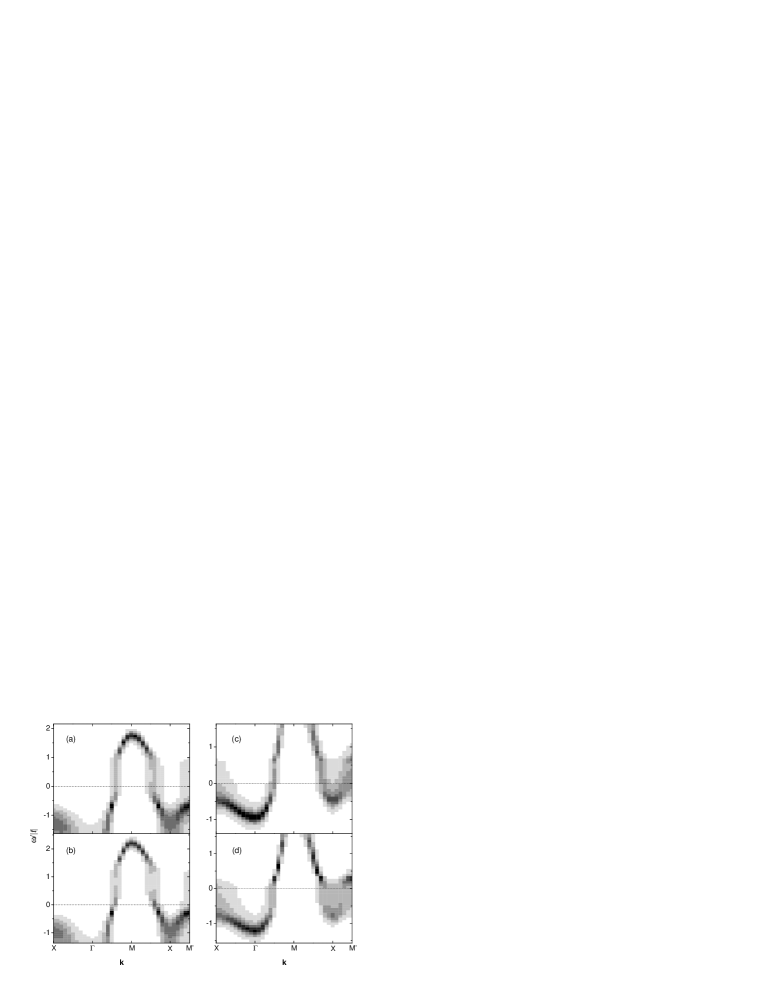
Figure 7: The dispersion of maxima of the spectral function in the $t$-$t^{\prime}$-$U$ model on a 20$\times$20 lattice for $t=-U/8$, $t^{\prime}/t=-0.3$, $T=0.001U$, $\eta=0.02U$, $\mu=0.1U$ (a), $0.05U$ (b), $0.9U$ (c), and $0.95U$ (d). Here darker areas correspond to larger intensities. The points X, $\Gamma$, M, and M’ correspond to the momenta $(\pi,0)$, $(0,0)$, $(\pi,\pi)$, and $(\pi/2,\pi/2)$, respectively.

IV The $t$-$t^{\prime}$-$U$ model

Now let us consider the $t$-$t^{\prime}$-$U$ model with the initial electron dispersion $t_{\bf k}=2t[\cos(k_{x})+\cos(k_{y})]+4t^{\prime}\cos(k_{x})\cos(k_{y})$. Both for the case of hole and electron doping the ratio $t^{\prime}/t=-0.3$ of the hopping constants for the next-nearest and nearest neighbors is accepted. Korshunov For both cases the spectral function and the dispersion of quasiparticle peaks near the Fermi level are shown in Figs. 6 and 7. As in the case of the $t$-$U$ model, at half-filling the spectrum of the $t$-$t^{\prime}$-$U$ model contains four well separated bands. Also in analogy with the former model a dispersive feature and a pseudogap appear near the Fermi level at a certain level of doping. However, in the case of the $t$-$t^{\prime}$-$U$ model the obvious asymmetry of the hole and electron doping stands out – the new feature and the pseudogap are less pronounced in the case of electron doping. This is also apparent from the comparison of Figs. 7a and c. Such behavior is a consequence of the asymmetry in the filling dependence of ${\rm Im}K(\omega)$ – for identical offsets from $\mu=U/2$ the sharp minima which are similar to those shown in Fig. 2b are more intensive in the case of hole doping than for electron doping. This asymmetry is connected with the contribution of the second term on the right-hand side of Eq. (9) to ${\rm Im}K(\omega)$.

Figure 7 demonstrates the dispersions of the new band and of the lower (upper) inner band in the case of hole (electron) doping, the inner band being located above (below) the Fermi level. The pseudogap between these bands becomes more pronounced with increasing $\bar{n}$ in the case of electron doping (cf. Figs. 7c and d). Similarly to the $t$-$U$ model, for the hole-doped case the magnitude of the pseudogap observed in photoemission decreases with increasing the hole doping (see Figs. 7a and b), while for the electron-doped case this magnitude increases with increasing the electron doping (see Figs. 7c and d).

Also as for the $t$-$U$ model, shapes of the spectral function and quasiparticle dispersions calculated in the $t$-$t^{\prime}$-$U$ model in the one-loop approximation are similar to those obtained in the cluster methods, provided that doping or temperature are high enough to ensure a short magnetic correlation length (cf. Fig. 6 with Fig. 2 in Ref. Senechal, and with Fig. 5a in Ref. Kyung, ). Again the most important difference between these two groups of results is a larger spectral intensity in the upper inner band near $(0,0)$ for the hole-doped case and in the lower inner band near $(\pi,\pi)$ for the electron-doped case in the one-loop approximation.

V Conclusion

In the present work the diagram technique was used for the investigation of the energy spectra of the $t$-$U$ and $t$-$t^{\prime}$-$U$ Hubbard models at a departure from half-filling. The one-loop approximation was applied which in the used diagram approach is a successive improvement to the Hubbard-I approximation. In agreement with results of Monte-Carlo simulations and cluster methods at half-filling the obtained spectra of the models contain four bands. The four-band structure persists also for some departure from half-filling. Additionally in these conditions a new narrow band of quasiparticle states arises near the Fermi level. The band energy is maximum near the boundary of the magnetic Brillouin zone. The dispersion of the band is much larger in the direction $(\pi/2,\pi/2)-(0,0)$ than along the boundary of the magnetic Brillouin zone $(\pi,0)-(0,\pi)$. The width of the band is of the order of the superexchange constant and decreases with increasing doping. By these properties the new band resembles the spin-polaron band of the $t$-$J$ model. For moderate doping the intensities of maxima in the new band and in one of the inner bands of the four-band structure decrease as the Fermi level is approached. As a consequence a pseudogap arises in the spectrum near the Fermi level. With hole doping the magnitude of the pseudogap observed in photoemission decreases and eventually the pseudogap disappears in agreement with experimental observations. With electron doping the magnitude of the photoemission pseudogap increases. Shapes of the spectral function and quasiparticle dispersions calculated in the one-loop approximation are similar to those obtained by Monte-Carlo simulations and cluster methods, provided that doping or temperature are high enough to ensure a short magnetic correlation length.

References

- (1) A. Moreo, S. Haas, A. W. Sandvik, and E. Dagotto, Phys. Rev. B 51, 12045 (1995); R. Preuss, W. Hanke, and W. von der Linden, Phys. Rev. Lett. 75, 1344 (1995).
- (2) C. Gröber, R. Eder, and W. Hanke, Phys. Rev. B 62, 4336 (2000).
- (3) T. Maier, M. Jarrell, T. Pruschke, and M. H. Hettler, Rev. Modern Phys. 77, 1027 (2005).
- (4) M. Aichhorn, E. Arrigoni, M. Potthoff, and W. Hanke, cond-mat/0511460 (unpublished).
- (5) A.-M. S. Tremblay, B. Kyung, and D. Sénéchal, Fizika Nizkikh Temperatur 32, 561 (2006).
- (6) F. Mancini and A. Avella, Adv. Phys. 53, 537 (2004); S. Onoda and M. Imada, J. Phys. Chem. Solids 63, 2225 (2002).
- (7) Yu. A. Izyumov, N. I. Chaschin, D. S. Alexeev, and F. Mancini, Eur. Phys. J. B 45, 69 (2005).
- (8) R. O. Zaitsev, ZhETF 70, 1100 (1976) [Sov. Phys. JETP 43, 574 (1976)]; Yu. A. Izyumov and B. M. Letfulov, J. Phys: Cond. Mat. 1, 8905 (1990); A. M. Shvaika, Phys. Rev. B 62, 2358 (2000);
- (9) Yu. A. Izyumov and Yu. N. Skryabin, Statistical Mechanics of Magnetically Ordered Systems, (Consultants Bureau, New York 1988).
- (10) S. G. Ovchinnikov and V. V. Valkov, Hubbard operators in the theory of strongly correlated electrons, (Imperial College Press, London, 2004).
- (11) M. I. Vladimir and V. A. Moskalenko, Teor. Mat. Fiz. 82, 428 (1990) [Theor. Math. Phys. 82, 301 (1990)]; S. I. Vakaru, M. I. Vladimir and V. A. Moskalenko, Teor. Mat. Fiz. 85, 248 (1990) [Theor. Math. Phys. 85, 1185 (1990)]; V. A. Moskalenko, P. Entel and D. F. Digor, Phys. Rev. B 59, 619 (1999).
- (12) W. Metzner, Phys. Rev. B 43, 8549 (1991).
- (13) S. Pairault, D. Sénéchal and A.-M. S. Tremblay, Eur. Phys. J. B 16, 85 (2000).
- (14) A. Sherman, Phys. Rev. B 73, 155105 (2006); cond-mat/0602537 (unpublished).
- (15) E. Dagotto, Rev. Modern Phys. 66, 763 (1994); Yu. A. Izyumov, Usp. Fiz. Nauk 167, 465 (1997) [Phys.-Usp. (Russia) 40, 445 (1997)].
- (16) M. M. Korshunov and S. G. Ovchinnikov, Fiz. Tverd. Tela (Leningrad) 43, 399 (2001) [Phys. Sol. State 43, 416 (2001)]; A. Macridin, M. Jarrel, T. Maier, and G. A. Sawatzky, Phys. Rev. B 71, 134527 (2005).
- (17) R. Kubo, J. Phys. Soc. Jpn. 17, 1100 (1962).
- (18) J. Hubbard, Proc. R. Soc. London, Ser. A 276, 238 (1963).
- (19) A. A. Abrikosov, L. P. Gor’kov, and I. E. Dzyaloshinskii, Methods of Quantum Field Theory in Statistical Physics, (Pergamon Press, New York, 1965).
- (20) D. Sénéchal and A.-M. S. Tremblay, Phys. Rev. Lett. 92, 126401 (2004).
- (21) B. Kyung, S. S. Kancharla, D. Sénéchal, A.-M. S. Tremblay, M. Civelli, and G. Kotliar, cond-mat/0502565 (unpublished).
- (22) A. Macridin, M. Jarrell, T. Maier, P. R. C. Kent, and E. D’Azevedo, cond-mat/0509166 (unpublished).
- (23) A. Damascelli, Z. Hussain, and Z.-X. Shen, Rev. Modern Phys. 75, 473 (2003).
- (24) A. Sherman and M. Schreiber, Phys. Rev. B 50, 12887 (1994); Physica C 303, 257 (1998); Eur. Phys. J. B 32, 203 (2003).
- (25) H. Shimahara and S. Takada, J. Phys. Soc. Jpn. 60, 2394(1991).
- (26) B. Keimer, N. Belk, R. J. Birgeneau, A. Cassanho, C. Y. Chen, M. Greven, M. A. Kastner, A. Aharony, Y. Endoh, R. W. Erwin, and G. Shirane, Phys. Rev. B 46, 14034 (1992).