Nonanalytic corrections to the specific heat and susceptibility of a non-Galilean-Invariant Two-Dimensional Fermi Liquid

Abstract

We consider the leading non-analytic temperature dependence of the specific heat and temperature and momentum dependence of the spin susceptibility for two dimensional fermionic systems with non-circular Fermi surfaces. We demonstrate the crucial role played by Fermi surface curvature. For a Fermi surface with inflection points, we demonstrate that thermal corrections to the uniform susceptibility in $D=2$ change from $\chi_{s}\propto T$ to $\chi_{s}\propto T^{2/3}$ for generic inflection points, and to $\chi_{s}\propto T^{1/2}$ for special inflection points along symmetry directions. Errors in previous work are corrected. Application of the results to $Sr_{2}RuO_{4}$ is given.

I Introduction

L. D. Landau’s ”Fermi liquid theory” provides a robust and accurate description of the leading low temperature, long wavelength behavior of a wide range of systems of interacting fermions in two and three spatial dimensions. In Landau’s original work Landau57 it was assumed that the temperature ($T$) and momentum ($q$) corrections to the leading Fermi liquid behavior were analytic functions of $(T/T_{F})^{2}$ and $(q/k_{F})^{2}$, with the Fermi momentum $k_{F}$ set by the inter-particle spacing and the Fermi temperature $T_{F}\sim v_{F}k_{F}$ with $v_{F}$ a typical measured electron velocity. However, subsequent work revealed that in dimensions $d=2$ and $d=3$ the leading temperature and momentum dependences of measurable quantities including the specific heat and spin susceptibility are in fact non-analytic functions of $T^{2}$ and $q^{2}$. The nonanalyticities have been studied in detail for Galilean-invariant systems (spherical Fermi surface or circular Fermi line) (see Ref  Chubukov06, for a list of references). In this paper we extend the analysis to a more general class of systems, still described by Fermi liquid theory but with a Fermi surface of arbitrary shape.

The extension is of interest in order to allow comparisons to systems such as $Sr_{2}RuO_{4}$ Bergemann03 and quasi-one-dimensional organic conductors organic , in which lattice effects are important. The extension also provides further insight into a fundamental theoretical issue: a crucial finding of the previous analysis Chubukov05 ; Chubukov06 was that for two dimensional systems the non-analytical term in the specific heat coefficient $\delta C(T)/T\propto T$ arise solely from ”backscattering” processes at any strength of fermion-fermion interaction. For the spin susceptibility, the situation is more complex: in addition to the backscattering contributions to $\delta\chi_{s}(T)\propto T$ and $\delta\chi_{s}(q)\propto q$ there are contributions of third and higher order in the interaction which involve non-backscattering processes ch_masl_latest . If the interaction is not too strong the backscattering terms dominate.

Unlike scattering at a general angle, the kinematics of backscattering is effectively one-dimensional, and depends sensitively on the shape of the Fermi surface. We shall show that the crucial parameter is the Fermi surface curvature, and that for two dimensional systems in which the Fermi surface possesses an inflection point, the power laws change from $\left|(T,q)\right|$ to $\left|(T,q)^{1/2}\right|$ or $\left|(T,q)^{2/3}\right|$ according to whether the inflection point is or is not along a reflection symmetry axis of the material. Similar effects occur in three dimensional systems, but the effects will be weaker as the singularities there are only logarithmic.

The importance of the Fermi surface geometry was previously noted by Fratini and Guinea, who showed that the presence of inflection points changes the power law for the spin susceptibility $\chi_{s}(T)$ Fratini02 . However, we believe that their calculation treated the kinematics of the backscattering incorrectly; as a result, they found that, in $2D$, the presence of the inflection point changes the temperature dependence only by a logarithm, from $\chi_{s}(T)\propto T$ to $\chi_{s}(T)\propto T\log T$, instead of the $T^{\left(\frac{1}{2},\frac{1}{3}\right)}$ found here.

The paper is organized as follows. Section II introduces the model and defines notation. In Section III, we demonstrate the physical origin of the results, via a calculation of the long range dynamical correlations of a Fermi liquid. Section IV presents results for the specific heat of a multiband system. In Section V we calculate the nonanalyticities in the momentum and temperature dependence of $\chi$. Section VI shows how new power laws emerge for Fermi surfaces with inflection points, and why one-dimensionality affects the powers. Section VII presents estimates of the size of the nonanalytic terms in $Sr_{2}RuO_{4}$. Section VIII is a conclusion.

II Model

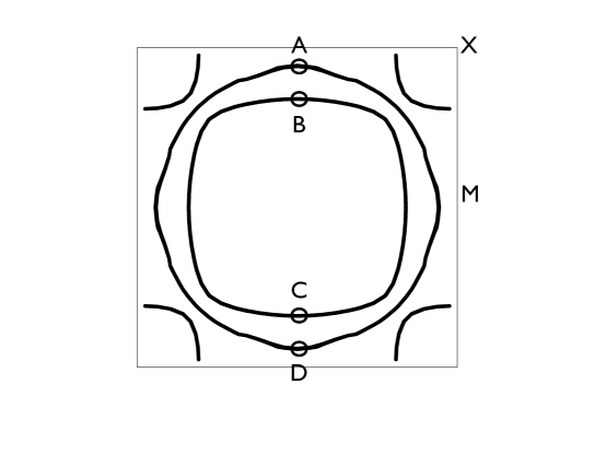
Figure 1: Fermi surface of $Sr_{2}RuO_{4}$ computed from tight binding parameters deduced from quantum oscillation measurements Bergemann03 , with a few ”parallel tangents” points indicated by letters A,B,C,D and the Brillouin zone points $M=(\pi,0)$ and $X=(\pi,\pi)$ also noted.

We study fermions moving in two dimensions in a periodic potential. As discussed at length in Ref. [Chubukov06, ], because we are concerned with the low $T$ properties of a Fermi liquid we may adopt a quasiparticle picture. Lifetime effects are not important, and the quasiparticle weight ($z$) factors may be absorbed in interaction constants. We may therefore consider several bands, labeled by band index $a$, of quasiparticles moving with (renormalized) dispersion $\varepsilon_{p}^{a}$. The Fermi surfaces are defined by the condition $\varepsilon_{\mathbf{k}}^{a}=\mu$; an example is shown in Fig 1. We parameterize the position at the Fermi surface by a coordinate $s^{a}$. For vectors $\mathbf{k}$ near a particular Fermi surface point $\mathbf{k}_{F}$ we will write

$$\varepsilon_{\mathbf{k}}^{a}-\mu=v_{F}^{a}(s^{a})\left(k_{\|}+\frac{k_{\bot}^{2}}{2k_{0}(s^{a})}\right)$$ (1)

with $v_{F}(s^{a})=\left|\partial\varepsilon_{\mathbf{k}}^{a}/\partial\mathbf{k}\right|$ the Fermi velocity at the point $(s^{a})$ and the components of $\mathbf{k}$ parallel and perpendicular to the Fermi velocity (Fermi surface normal) given by

$$k_{\|} =\left(\mathbf{k}-\mathbf{k}_{F}\right)\cdot\widehat{\mathbf{v}}_{F}(s^{a})$$ (2)

$$k_{\bot} =\left(\mathbf{k}-\mathbf{k}_{F}\right)\times\widehat{\mathbf{v}}_{F}(s^{a})$$ (3)

$k_{0}^{-1}(s^{a})$ is the curvature of the Fermi surface at the point $s^{a}$. For a circular Fermi surface, $k_{0}=k_{F}$ independent of $s$; but in general $k_{0}\neq k_{F}$ and both depend on $s$.

It is sometimes convenient to use the variables $\varepsilon_{k}$ and $\theta_{k}$, where $\theta_{k}$ is the angle determining the direction of the Fermi velocity ${\bf v}_{F}(k)=\partial\varepsilon_{k}/\partial{\bf k}$ relative to some fixed axis. Eq 1 shows that the Jacobean of the transformation is

$$d^{2}k=\frac{k_{0}(k)}{v_{F}(k)}d\varepsilon_{k}d\theta_{k}.$$ (4)

In a non-Galilean-invariant system the Fermi surface may contain inflection points at which the curvature vanishes, i.e. $k_{0}\rightarrow\infty$. If the inflection point does not lie on an axis of reflection symmetry of the Brillouin zone, the dispersion (measured in terms of the difference of the momentum from an inflection point) is

$$\varepsilon_{\mathbf{k}}-\mu=v_{F}\left(k_{\|}+\frac{k_{\bot}^{3}}{k^{2}_{1}}\right)$$ (5)

However, if the inflection point lies on a symmetry axis, then only even powers in $k_{\bot}$ may occur and

$$\varepsilon_{\mathbf{k}}-\mu=v_{F}\left(k_{\|}+\frac{k_{\bot}^{4}}{k^{3}_{2}}\right)$$ (6)

Here $k_{1}$ and $k_{2}$ are coefficients expected in general to be $\sim k_{F}$.

The fermions interact. We assume that the $T\rightarrow 0$, long wavelength properties are described by the Fermi liquid theory, so that at low energies the interactions may be parameterized by the fully reducible Fermi surface to Fermi surface scattering amplitude $\Gamma_{\alpha,\beta,\gamma\delta}(k,p;k,p)$. For particles near the Fermi surface, $|{\bf k}|,|{\bf p}|\approx k_{F}$, and $\Gamma$ depends on the angle $\theta$ between ${\bf k}$ and ${\bf p}$ and on the band indices $a$ (for $k$) and $b$ (for $p$). Backscattering corresponds to $\theta=\pi$. It is often useful to decompose $\Gamma_{\alpha,\beta;\gamma,\delta}(\pi)$ into charge and spin components

$$\Gamma^{ab}_{\alpha,\beta;\gamma,\delta}(\pi)=\Gamma^{ab,c}\delta_{\alpha\gamma}\delta_{\beta\delta}+\Gamma^{ab,s}{\bf\sigma}_{\alpha\gamma}{\bf\sigma}_{\beta\delta}$$ (7)

It is also instructive to make contact with second order perturbation theory for a model in which the particles are subject to a spin-independent interaction

$$H_{int}=\sum_{\mathbf{q}}U(\mathbf{q})\rho_{\mathbf{q}}\rho_{-\mathbf{q}}$$ (8)

with charge density operator

$$\rho_{\mathbf{q}}=\sum_{\mathbf{p}\alpha}c_{\mathbf{p+q},\alpha}^{{\dagger}}c_{p,\alpha}$$ (9)

The leading perturbative result is then

$$\Gamma^{c}=U(0)-\frac{U(2k_{F})}{2},~{}~{}~{}\Gamma^{s}=-\frac{U(2k_{F})}{2}$$ (10)

If the interaction is local and only one band is relevant, i.e., $U(q)=U$, $\Gamma^{c}=-\Gamma^{s}=U/2$, and

$$\Gamma_{\alpha,\beta;\gamma,\delta}(\pi)=U\left(\delta_{\alpha\gamma}\delta_{\beta\delta}-\delta_{\alpha\delta}\delta_{\beta\gamma}\right)$$ (11)

III Physical Origin of Nonanalyticities; role of curvature

Previous studies of the isotropic case demonstrated Chubukov05 ; Chubukov06 that the nonanalyticities in the specific heat and spin susceptibility arise from the long spatial range dynamical correlations characteristic of Fermi liquids. These are of two types. One involves slow ($|\Omega|<v_{F}q$) long wavelength fluctuations and is expressed mathematically in terms of the long wavelength limit of the polarizibility $\delta\Pi_{LW}\equiv lim_{q\rightarrow 0}\Pi(q,\Omega)-\Pi(q,0)\sim\left|\Omega\right|/q$. The $1/q$ behavior of polarizibility gives rise to a long-range correlation between fermions which decays as $|\Omega|/r$ at distances $1\ll rk_{F}<E_{F}/|\omega|$. The other involves processes with momentum transfer $q\approx 2p_{F}$, and is expressed mathematically in terms of the polarizibility $\delta\Pi\equiv\Pi(q,\Omega)-\Pi(2k_{F},\Omega)\sim\Omega/\sqrt{2k_{F}-q}$ (for $|\Omega|<2k_{F}-q$. The $1/\sqrt{2k_{F}-q}$ behavior of $\delta\Pi$ gives rise to an oscillation with a slowly decaying envelope, $\cos(2k_{F}r-\pi/4)|\Omega|/\sqrt{r}$ , again at distances $1\ll rp_{F}<E_{F}/|\omega|$ and again leading to singular behavior. We now compute these processes in the multiband model defined above, and then show how they affect thermodynamic variables.

Consider the long wavelength process first. The non-analyticity comes from a particle-hole pair excitation in which both particle and hole are in the same band, and have momenta in the vicinity of Fermi surface points $s_{a}^{*}$ satisfying $\vec{v}_{F}(s_{a}^{*})\cdot{\vec{q}}=0$. Choosing one of these points as the origin of coordinates we have

$$\delta\Pi^{aa}_{s_{a}^{*}} \equiv \Pi_{s_{a}^{*}}(q,\Omega)-\Pi_{s_{a}^{*}}(q,0)=T\sum_{n}\int\frac{dk_{\|}dk_{\bot}}{(2\pi)^{2}}\frac{1}{i\omega_{n}-v_{F}(s_{a}^{*})\left(k_{\|}+\frac{(k_{\bot}-q/2)^{2}}{2k_{0}(s_{a}^{*})}\right)}$$ (12)

$$\times \left(\frac{1}{i\omega_{n}+i\Omega_{n}-v_{F}(s_{a}^{*})\left(k_{\|}+\frac{(k_{\bot}+q/2)^{2}}{2k_{0}(s_{a}^{*})}\right)}-\frac{1}{i\omega_{n}-v_{F}(s_{a}^{*})\left(k_{\|}+\frac{(k_{\bot}+q/2)^{2}}{2k_{0}(s_{a}^{*})}\right)}\right)$$

Performing the integral over $k_{\|}$ and the Matsubara sum as usual yields

$$\delta\Pi^{aa}_{s_{a}^{*}}=\int\frac{dk_{\bot}}{2\pi}\frac{1}{2\pi v_{F}(s_{a}^{*})}\frac{i\Omega}{i\Omega-\frac{v_{F}(s_{a}^{*})k_{\bot}q}{k_{0}(s_{a}^{*})}}$$ (13)

We see that for the part of $\delta\Pi$ which is even in $\Omega$ the integral is indeed dominated by $k_{\bot}\sim\Omega k_{0}(s_{a}^{*})/v_{F}(s_{a}^{*})$, so the approximation of expanding near this point is justified, and we obtain the nonanalytic long wavelength contribution as a sum over all Fermi points $s_{a}^{*}$ satisfying $\vec{v}_{F}(s_{a}^{*})\cdot\vec{q}=0$ with coefficients determined by the local Fermi velocity and local curvature:

$$\delta\Pi^{aa}_{LW}(q,\Omega)=\frac{\left|\Omega\right|}{q}\left(\sum_{s_{a}^{*}}\frac{k_{0}(s_{a}^{*})}{4\pi v_{F}^{2}(s_{a}^{*})}\right)$$ (14)

For a circular Fermi surface, two points satisfy $\vec{v}_{F}(s_{a}^{*})\cdot\vec{q}=0$, $k_{0}=k_{F}$ and Eq. (14)  reduces to the familiar result $k_{F}|\Omega|/(2\pi v^{2}_{F}q)$. If the curvature vanishes, then use of Eqs (5) or (6) in Eq (12) yields a $\delta\Pi_{LW}\sim\left(\Omega/q\right)^{1/2,1/3}$ respectively.

We next consider the ”$2k_{F}$” process. Here the situation is a little different. The singularities in general come from processes connecting two Fermi points with parallel tangents (the importance of parallel tangents points has been noted in other contexts Altshuler95 )–for example the points $A,B$ or $A,C$ shown in Fig 1. For a given vector ${\bf q}$ we denote as ${\bf Q}$ the closest vector which is parallel to ${\bf q}$ and connects two ”parallel tangents” points. Symmetry ensures that the leading dependence of $\delta\Pi^{ab}_{Q}=\Pi({\bf q})-\Pi({\bf Q})$ involves only the $q_{\|}=({\bf q}-{\bf Q})\cdot{\bf Q}/|{\bf Q}|$. Labeling the initial and final of the two Fermi points connected by $Q$ as $s_{1,2}$ and noting that for systems with inversion symmetry the points come in pairs symmetric under interchange to the band indices we have

$$\delta\Pi^{ab}_{Q}\equiv\Pi({\bf q},\Omega)-\Pi({\bf Q},0)=T\sum_{n}\int\frac{dk_{\|}dk_{\bot}}{(2\pi)^{2}}\frac{1}{i\omega_{n}-v_{F}(s_{1})\left(k_{\|}+\frac{k_{\bot}^{2}}{2k_{0}(s_{1})}\right)}\times$$

$$\left(\frac{1}{i\omega_{n}+i\Omega_{n}-v_{F}(s_{2})\left(k_{\|}+q_{\|}+\frac{k_{\bot}^{2}}{2k_{0}(s_{2})}\right)}-\frac{1}{i\omega_{n}-v_{F}(s_{2})\left(k_{\|}+\frac{k_{\bot}^{2}}{2k_{0}(s_{2})}\right)}\right)+(1\leftrightarrow 2)$$ (15)

Here the sign of $v_{F}$ and $k_{0}$ becomes important. For two points ”on the same side” of the Fermi surface (e.g. points $A$ and $B$ in Fig 1) the two velocities and the two curvatures have the same sign (a change of $k_{\|}$ either increases or decreases both energies), the integrations proceed as in the analysis of Eq (12), and the different position of the $q$ means that to the order of interest there is no singular non-analytical term. On the other hand, if the two velocities have opposite sign (e.g. points $A$, $C$ in Fig 1) then after integrating over $k_{\|}$ and $k_{\bot}$ we obtain (for $\Omega>0$)

$$\delta\Pi_{Q}=\frac{\sqrt{k_{avg}}}{\left|4v_{F1}v_{F2}\right|}T\sum_{\omega_{n}>0\hskip 1.4457ptor\hskip 1.4457pt\omega_{n}<-\Omega}\frac{sgn(\omega)}{\sqrt{\frac{2i\omega}{v_{avg}}+\frac{i\Omega}{v_{F2}}-q_{\|}}}+\left(1\leftrightarrow 2\right)$$ (16)

Here $v_{F1}=v_{F}(s_{1}),~{}v_{F2}=v_{F}(s_{2})$, and

$$\frac{1}{k_{avg}} = \frac{1}{2}\left(\frac{1}{k_{0}(s_{1})}+\frac{1}{k_{0}(s_{2})}\right)$$ (17)

$$\frac{1}{v_{avg}} = \frac{1}{2}\left(\frac{1}{\left|v_{F1}\right|}+\frac{1}{\left|v_{F2}\right|}\right)$$ (18)

Completing the evaluation yields

$$\delta\Pi_{Q}=\frac{\sqrt{k_{avg}}}{4\pi\left|(v_{F1}\right|+\left|v_{F2}\right|)}~{}\left(\sqrt{q_{\|}+\frac{i\Omega}{|v_{F1}|}}+\sqrt{q_{\|}-\frac{i\Omega}{|v_{F1}|}}+1\leftrightarrow 2\right)$$ (19)

The singular $|\Omega|/\sqrt{q}$ behavior of the dynamic $\delta\Pi_{Q}$ only holds when $q_{\|}<0$ and is obtained by expanding (19) in $\Omega/q_{\|}$. On the contrary, the singular behavior of the static $\Pi_{Q}\propto\sqrt{q_{\|}}$ holds at $q_{\|}>0.$ The dynamic part of $\Delta\Pi_{Q}$ behaves as $\Omega^{2}/(q_{\|})^{3/2}$ at $q_{\|}>0$.

Figure 2: One of the two second-order diagrams for the free energy, which give the non-analytic contribution to the specific heat (from Ref.Chubukov06, ). Here $\Gamma$ is the (unsymmetrized) fully renormalized Fermi surface to Fermi surface scattering amplitude.

IV Specific Heat

This section treats the non-analyticity in the specific heat. The Galilean-invariant case studied previously is simple enough that the corrections can be evaluated, with no approximations beyond the usual ones of Fermi Liquid theory Chubukov06 . The evaluation confirms that in two dimensions the non-analytical contributions to the specific heat involve only the backscattering amplitude $\Gamma(\pi)$. In work prior to that reported in Ref [Chubukov06, ] this conclusion was reached by approximate calculations in which it was assumed that the non-analytical contributions were governed by the backscattering amplitude only, and then the assumption was shown a fortiori to be consistent. In the non-Galilean-invariant case of interest here, a complete analysis along the lines of Ref [Chubukov06, ] is not possible. We will follow earlier work and assume that the effects arise only from backscattering processes, and then show that the assumption is self consistent. We specialize for ease of writing to a momentum-independent vertex $\Gamma$ (see (11)), but keep band indices. For a two-dimensional system the diagram which gives the nonanalytic term in the thermodynamic potential $\Xi$ is Chubukov06 shown in Fig 2. We may write the resulting diagram schematically as

$$\Xi=-\frac{1}{2}\sum_{abcd}\int(dqd\Omega)\Gamma_{abcd}^{2}\Pi_{ab}(q,\Omega)\Pi_{cd}(q,\Omega)$$ (20)

Now, singularities leading to non-analytical terms may arise for $q\rightarrow 0$, in which case we must consider only the intraband contribution to $\Pi$, and $q\rightarrow Q$, where $Q$ is one of the ”parallel tangents” vectors mentioned in the previous section, in which case the band indices of polarizabilities may be different. Let us consider first the small $q$ singularities. We have

$$\Xi_{LW}=-\frac{1}{2}\sum_{ab}\int(dqd\Omega)\Gamma_{aabb}^{2}\Pi_{aa}(q,\Omega)\Pi_{bb}(q,\Omega)$$ (21)

Substituting from Eq (14) gives

$$\Xi_{LW}=-\frac{1}{2}T\sum_{\Omega}\int\frac{qdqd\theta}{(2\pi)^{2}}\sum_{ab}\Gamma_{aabb}^{2}\frac{\Omega^{2}}{q^{2}}\frac{k_{0}^{a}(\theta)k_{0}^{b}(\theta)}{(4\pi)^{2}v_{F,a}^{2}v_{F,b}^{2}}$$ (22)

The integral over $q$ is logarithmic and is cut by $\Omega$; the analytical continuation and integral of frequencies may then be performed and we obtain

$$\left.\frac{\delta C}{T}\right|_{LW}=-\frac{3\zeta(3)}{\pi^{3}}\sum_{ab}\int\frac{d\theta}{2\pi}\frac{\Gamma_{aabb}^{2}k_{0}^{a}(\theta)k_{0}^{b}(\theta)}{v_{F,a}^{2}v_{F,b}^{2}}$$ (23)

We now turn to the parallel tangents part of the calculation, finding

$$\Xi_{Q}=-\frac{1}{2}\sum_{ab}\int(dqd\Omega)\Gamma_{abba}^{2}\Pi_{ab}(Q+q,\Omega)\Pi_{ba}(Q+q,\Omega)$$ (24)

Note that the symmetry of the vertex means that $\Gamma_{abba}^{2}=\Gamma_{aabb}^{2}$. Again substituting $\Delta\Pi_{Q}$ instead of $\Pi_{ab}(Q+q,\Omega)$ and evaluating the integrals explicitly we find  comm_2 (note that to obtain the non-analytical behavior it is sufficient to expand $\delta\chi_{Q}$ for $|\Omega|<<q$)

$$\Xi_{Q}=-\frac{1}{2}\sum_{ab}\Gamma_{abba}^{2}T\sum_{\Omega}\int\frac{dq_{\|}dq_{\bot}}{(2\pi)^{2}}\frac{\Omega^{2}}{(4\pi)^{2}v_{Fa}^{2}v_{Fb}^{2}}\frac{k_{avg}}{|q_{\|}|}$$ (25)

Now noting that $k_{avg}=k_{0}^{a}k_{0}^{b}/(k_{0}^{a}+k_{0}^{b})$ and that $dq_{\bot}=(k_{0}^{a}+k_{0}^{b})d\theta$ we see that $\Xi_{Q}$ and $\Xi_{LW}$ give identical contributions despite the apparently different kinematics.

Adding the two contributions, we obtain

$$\frac{\delta C}{T}=-\frac{3\zeta(3)}{2\pi^{3}}\sum_{ab}\int\frac{d\theta}{2\pi}\frac{\Gamma_{aabb}^{2}k_{0}^{a}(\theta)k_{0}^{b}(\theta)}{v_{F,a}^{2}v_{F,b}^{2}}$$ (26)

Note that the integrals over the Fermi surface contain $k^{2}_{0}=k^{2}_{0}(\theta_{k})$ rather than the product of two $k_{0}$ factors at different points along the Fermi surface. This is a direct consequence of the fact that only backscattering contributes to (40) and (41). For a one band model with an isotropic Fermi surface, Eq. (26) reduces to the result in Chubukov05 . For a generic interaction, the calculation goes through as before with $\Gamma^{2}_{aabb}$ replaced the components of the fully renormalized, symmetrized Fermi surface to Fermi surface backscattering amplitude so that

$$\frac{\delta C}{T}=-\frac{3\zeta(3)}{2\pi^{3}}\sum_{ab}\int\frac{d\theta}{2\pi}\frac{\left(\Gamma^{ab,c}(\pi)^{2}+3\Gamma^{ab,s}(\pi)\right)^{2}k_{0}^{a}(\theta)k_{0}^{b}(\theta)}{v_{F,a}^{2}v_{F,b}^{2}}$$ (27)

V Susceptibility

Figure 3: Relevant second-order diagrams for the spin and charge susceptibilities (ferm Ref.Chubukov05 ). The last two diagrams are non-zero only for the charge susceptibility.

V.1 Overview

This section presents calculations of the non-analytical momentum and temperature dependence of the spin susceptibility of a two dimensional non-Galilean-invariant Fermi liquid system. with a Fermi surface without inflection points. In contrast to the specific heat, there are two classes of contributions to the nonalnayticities in the susceptibility ch_masl_latest . One is of second order in the fullly renormalized interaction amplitudes, involves only the backscattering, and is treated here. The other, which we do not study here, is of third and higher orders, and involve averages of the interaction function over a wide range of angles (analogously to similar contributions to the specific heat of a three dimensional Fermi liquid Chubukov06 ). The former process is dominant at weak coupling, and involves an integral of the square of the curvature over the Fermi arc. The latter process has a less singular dependence on the curvature.

Even to the order at which we work, many diagrams contribute (see Fig 3); we evaluate one in detail to illustrate the basic ideas behind the calculation and then simply present the result for the sum of all diagrams. Consider for definiteness the ”vertex correction” diagram – diagram 3 in Figure 3. The analytical expression corresponding to this diagram is (we use a condensed notation in which (dk) stands for an integral over momentum, normalized by $(2\pi)^{2}$, and a sum over the corresponding Matsubara frequency)

$$\delta\chi(q,0)=-4\sum_{ab}\int(dk)(dl)G^{a}(k+q)G^{a}(k)\Lambda^{ab}_{k}(l)G^{a}(k+l+q)G^{a}(k+l)$$ (28)

and $\Lambda$ is the product of the interaction vertices and internal polarization bubble:

$$\Lambda^{ab}_{k}(q)=\int(dp)\left(\Gamma^{aabb}(\theta)\right)^{2}G^{b}(p+q/2)G^{b}(p-q/2)]$$ (29)

where $\theta$ is the angle between ${\bf k}$ and ${\bf p}$, and we have used the fact that ${\bf k}$ and ${\bf p}$ are near the Fermi surface. A complete calculation in the Galilean-invariant case shows that, just as for the specific heat, the non-analytical momentum dependence of the susceptibility arises from the regions of small $l$ and $l\sim 2k_{F}$. We consider these in turn.

V.2 Small l

Here we choose a particular point $s_{k}$ on the Fermi surface and integrate over $\varepsilon_{k}$ and the corresponding frequency. We parametrize the position on the Fermi surface by the angle $\phi$ between ${\mathbf{v}}_{k}$ and ${\bf q}$ and use Eq 4. We adopt coordinates $l_{\|}$ and $l_{\bot}$ denoting directions parallel and perpendicular to ${\bf v}(s_{k})$ and obtain

$$\delta\chi_{LW}(q) = -\frac{4}{2\pi}\sum_{ab}\int\frac{d\theta_{k}k^{a}_{0}(\theta_{k})}{2\pi(v^{a}_{k})^{2}}\int\frac{dl_{\|}dl_{\bot}}{(2\pi)^{2}}T\sum_{\Omega}\frac{i\Omega}{\left({\bf v}^{a}_{k}\cdot{\bf q}\right)^{2}}\Lambda^{ab}_{k}(l_{\|},l_{\bot},\Omega)$$ (30)

$$\left(\frac{1}{\frac{i\Omega}{v^{a}_{k}}-{\hat{\bf v}}_{k}\cdot{\bf q}-l_{\|}}+\frac{1}{\frac{i\Omega}{v^{a}_{k}}+{\hat{\bf v}}_{k}\cdot{\bf q}-l_{\|}}-\frac{2}{\frac{i\Omega}{v^{a}_{k}}-{\hat{\bf v}}_{k}\cdot{\bf q}-l_{\|}}\right)$$

We may similarly evaluate $\Lambda$, proceeding from Eq (29). Choosing as origin the point ${\bf p}=-{\bf k}$, defining coordinates $p_{\|}$ and $p_{\bot}$ antiparallel and perpendicular to ${\bf v}_{k}$, integrating over $p_{\|}$ and the corresponding loop frequency gives

$$\Lambda^{ab}_{k}(l_{\|},l_{\bot},\Omega)=\frac{\Gamma^{aabb}(\pi)^{2}}{2\pi(v^{b}_{k})^{2}}\int\frac{dp_{\bot}}{2\pi}\frac{i\Omega}{\frac{i\Omega}{v^{b}_{k}}+l_{\|}-\frac{p_{\bot}l_{\bot}}{k^{b}_{0}}}$$ (31)

Viewed as a function of $l_{\|}$ the second line in Eq (30) decays rapidly ($\sim l_{\|}^{3}$) at large $l_{\|}$ and has poles only in the half plane $sgnIml_{\|}=sgn\Omega$. Evaluation of the $l_{\|}$ integral by contour methods, closing the contour in the half plane $sgnl_{\|}=-sgn\Omega$ shows that nonanalyticities can only arise from singularities of $\Lambda$. Reference to Eq (31) shows that these can only arise from momenta ${\bf p}$ satisfying ${\bf v}_{p}\cdot{\bf v}_{k}<0$. In the Galilean-invariant case the integral could be evaluated exactly; the resulting non-analytical terms were found to be determined by a very small region around ${\bf p}=-{\bf k}$, i.e., around $\theta=\pi$ in (29). Here we assume that this is the case, and show a fortiori that the assumption is consistent.

Performing the integral over $l_{\|}$ yields

$$\delta\chi_{LW}(q) = -4i\sum_{ab}\frac{(\Gamma^{aabb}(\pi))^{2}}{(2\pi)^{2}}\int\frac{d\theta_{k}k^{a}_{0}(k)}{2\pi(v^{a}_{k}v^{b}_{k})^{2}}T\sum_{\Omega}\int\frac{dl_{\bot}dp_{\bot}}{(2\pi)^{2}}\left(\frac{\Omega}{{\bf v}^{a}_{k}\cdot{\bf q}}\right)^{2}\text{sgn}\Omega$$ (32)

$$\left(\frac{1}{\frac{2i\Omega}{v_{avg}}-{\hat{\bf v}}_{k}\cdot{\bf q}-\frac{l_{\bot}p_{\bot}}{k^{b}_{0}}}+\frac{1}{\frac{2i\Omega}{v_{avg}}+{\hat{\bf v}}_{k}\cdot{\bf q}-\frac{l_{\bot}p_{\bot}}{k^{b}_{0}}}-\frac{2}{\frac{2i\Omega}{v_{avg}}-\frac{l_{\bot}p_{\bot}}{k^{b}_{0}}}\right)$$

with $v_{avg}$ defined in Eq 18. Performing the sum over frequency and rescaling each of $l_{\bot},p_{\bot}$ by $\sqrt{k^{b}_{0}}$ yields

$$\delta\chi_{LW}(q) = -\sum_{ab}\frac{\left(\Gamma^{aabb}(\pi)\right)^{2}}{8\pi^{3}}\int\frac{d\theta_{k}k^{a}_{0}k^{b}_{0}}{2\pi(v^{a}_{k}v^{b}_{k})^{2}}\int_{-\Lambda}^{\Lambda}\frac{dl_{\bot}dp_{\bot}}{(2\pi)^{2}}~{}\frac{v_{avg}^{3}}{(v^{a})^{2}}$$ (33)

$$\frac{\left(\Upsilon(l_{\bot},p_{\bot};{\hat{\bf v}}\cdot{\bf q})+\Upsilon(l_{\bot},p_{\bot};-{\hat{\bf v}}\cdot{\bf q})-2\Upsilon(l_{\bot},p_{\bot};0)\right)}{({\hat{\mathbf{v}}}_{k}\cdot{\bf q})^{2}}+...$$

with

$$\Upsilon(x,y;z)=(xy-z)^{2}\log|xy-z|$$ (34)

Eq (33) is based on an expansion for small $l_{\bot},p_{\bot}$. The integrals over these quantities are cut off by other physics above a cutoff scale $\Lambda$ which we have written as a hard cutoff. The ellipsis denotes other terms arising from physics at and beyond the cutoff scale, which lead to additional, regular contributions to $\delta\chi$ involving positive, even powers of $q$. Evaluation of Eq 33 yields (details are given in Appendix A)

$$\delta\chi_{LW}(q)=-\sum_{ab}\frac{\left(\Gamma^{aabb}(\pi)\right)^{2}\left|{\bf q}\right|}{48\pi^{3}}\int\frac{d\theta_{k}k^{a}_{0}k^{b}_{0}}{2\pi(v^{a}_{k})^{2}(v^{b}_{k})^{2}}\frac{v_{avg}^{3}}{(v^{a})^{2}}\left|{\hat{\mathbf{v}}}_{k}\cdot{\hat{q}}\right|+...$$ (35)

where $v_{k}=v_{F}(\theta_{k})$, $k_{0}=k_{0}(\theta_{k})$, ${\hat{\mathbf{v}}}_{k}\cdot{\hat{q}}=\cos(\theta_{k}-\theta_{q})$, and $\theta_{q}$ is the angle between the direction of ${\bf q}$ and the direction of $\theta=0$; the ellipsis again denotes analytical terms. We see that the non-analytical term is explicitly independent of the cutoff, confirming the consistency of our analysis. An alternative evaluation of $\delta\chi_{LW}(q)$ is presented in the Appendix  B.

For a circular Fermi surface, $k_{0}=k_{F}$, $v_{F}$ is a constant, and Eq. (35) reduces to the previously known result Chubukov05 . However, the previously published computations are arranged in a way which apparently does not invoke the curvature at all. In Appendix C we show that the previous method does in fact involve the curvature, and leads to results equivalent to those presented here.

V.3 $2p_{F}$ processes

To evaluate the contribution of $2p_{F}$ processes we could proceed from Eq (28) but expanding $\Lambda$ in ${\tilde{q}}=q-Q$, where, we remind, $Q=2k_{F}{\hat{q}}$. As before the products of $G$ produce an expression with all poles in the same half plane. Exploiting the non-analyticity of $\Pi({\bf q}+{\bf{\tilde{q}}},\Omega)$ we obtain an expression which has a nonanalytic part which evaluates to the same expression as Eq (35). Instead of presenting the details of this calculation, we present an alternative approach due to Belitz, Kirkpatrick, and Vojta bkv , in which one partitions the diagram into two ”triads”, using the explicit form of $\Lambda_{k}$

$$\delta\chi(q)=-4\sum_{ab}\int(dl)(dk_{1})(dk_{2})\Gamma^{aabb}(\theta)^{2}\left[G^{a}(k_{1}+q)G^{a}(k_{1})G^{a}(k_{1}+l)\right]\left[G^{b}(k_{2}+q)G^{b}(k_{2})G^{b}(k_{2}+l)\right]$$ (36)

where $\theta$ is the angle between ${\bf k}_{1}$ and ${\bf k}_{2}$. Choosing a particular point on the Fermi surface and evaluating the integral over $\varepsilon_{k_{1}}$ and the associated frequency yields ($q_{\|}$ is the component of ${\bf q}$ parallel to the direction chosen for $k_{1}$)

$$\delta\chi =-4\int\frac{k_{0}(\theta_{1})d\theta_{1}}{2\pi(v^{a})^{2}}\frac{\Omega}{({\bf v^{a}}\cdot{\bf q})}\left(\frac{1}{(\frac{i\Omega}{v^{a}}-l_{\|})}-\frac{1}{\frac{i\Omega}{v^{a}}-{\hat{\mathbf{v}}}\cdot{\mathbf{q}}-l_{\|})}\right)$$ (37)

$$\Gamma^{aabb}(\theta_{1})^{2}\left[G^{b}(k_{2}+q)G^{b}(k_{2})G^{b}(k_{2}+l)\right]$$

As in the previous calculation, singular contributions can only come from regions where $k_{2}$ is directed oppositely to $k_{1}$. Choosing as origin of $k_{2}$ the point diametrically opposite $k_{1}$, introducing parallel and perpendicular components as before and integrating over $k_{2\|}$, the associated frequency, and $l_{\|}$ we get

$$\delta\chi = \sum_{ab}4i\int\frac{k^{a}_{0}(\theta_{1})d\theta_{1}}{2\pi(v^{a})^{2}(v^{b})^{2}}\frac{\Gamma^{2}(\pi)}{(2\pi)^{2}}T\sum_{\Omega}\int\frac{dk_{\bot}dl_{\bot}}{(2\pi)^{2}}\left(\frac{\Omega^{2}\text{sgn}\Omega}{\left|({\bf v^{a}}\cdot{\bf q})({\bf v}^{b}\cdot{\bf q})\right|}\right)$$ (38)

$$\left(\frac{1}{\frac{2i\Omega}{v_{avg}}-{\hat{\mathbf{v}}}\cdot{\bf q}-\frac{l_{\bot}k_{\bot}}{k^{b}_{0}}}+\frac{1}{\frac{2i\Omega}{v_{avg}}+{\hat{\mathbf{v}}}\cdot{\bf q}-\frac{l_{\bot}k_{\bot}}{k^{b}_{0}}}-\frac{2}{\frac{2i\Omega}{v_{avg}}-\frac{l_{\bot}k_{\bot}}{k^{b}_{0}}}\right)$$

Eq (38) is seen to be of precisely the same form as Eq (32) and gives the same result; the only difference is the dependence on orbital index. Integrating over frequency and combining the results from small $q$ and $2k_{F}$ contributions gives an answer whose orbital dependent part depends on the velocities via the combination

$$\frac{v^{a}(v^{b})^{3}+(v^{a})^{3}v^{b}+2(v^{a})^{2}(v^{b})^{2}}{(v^{a}+v^{b})^{3}}\left({\hat{\mathbf{v}}}\cdot{\mathbf{q}}\right)=v_{avg}{\hat{\mathbf{v}}}\cdot{\bf q}$$ (39)

V.4 Final Result

Collecting the small $q$ and $2k_{F}$ contributions from all diagrams in Fig. 3 we find for the spin susceptibility

$$\delta\chi_{s}(q)=\sum_{ab}\frac{v_{avg}|q|}{6\pi^{3}}~{}\int_{0}^{2\pi}\frac{k^{a}_{0}(\theta_{k})k^{b}_{0}(\theta_{k})d\theta_{k}}{2\pi(v^{a})^{2}(v^{b})^{2}}(\Gamma^{ab,s}(\pi))^{2}\left|{\hat{\mathbf{v}}}\cdot{\hat{\mathbf{q}}}\right|$$ (40)

At $q=0$ and $T>0$, we have

$$\delta\chi_{s}(T)=\sum_{ab}\frac{T}{\pi^{3}}\int_{0}^{2\pi}\frac{d\theta_{k}k^{a}_{0}(\theta_{k})k^{b}_{0}(\theta_{k})}{2\pi(v^{a})^{2}(v^{b})^{2}}(\Gamma^{ab,s}(\pi))^{2}).$$ (41)

For an isotropic Fermi surface and one band, this again reduces to the result in Chubukov05 . To make contact with previous work, which considered a simplified interaction with indentical spin and charge components, $\Gamma^{ab,s}(\pi)$ has to be replaced by $\Gamma^{ab}(\pi)/2$. Higher order powers of $\Gamma$ do contribute to $|q|$ and $T$ terms in $\chi_{s}$, in distinction to $C(T)/T$, and at strong coupling, the non-analytic terms in the spin susceptibility are not expressed entirely via $\Gamma^{2}_{s}(\pi)$ ch_masl_latest . the terms of order $\Gamma^{3}$ have a less singular dependence on the curvature. At weak and moderate coupling, though, Eqs. (40) and (41) should be sufficient. Finally, for the charge susceptibility $\chi_{c}(q,T)$ non-analytic contributions from individual diagrams are all cancelled out: the full $\chi_{c}(q,T)$ is an analytic function of both arguments.

VI Fermi surfaces with Inflection Points

We see from Eq. (40) and (41) that as long as $k_{0}$ is finite all along the Fermi surface, the anisotropy of the Fermi surface affects the prefactors for $|q|$ and $T$ terms, but do not change the functional forms of the non-analytic terms in the specific heat and spin susceptibility. New physics, however, emerges when the Fermi surface develops inflection points at which $k_{0}(\theta_{k})$ diverges. Inflection points are a generic feature of realistic Fermi surfaces of two dimensional materials. In this section we show how inflection points emerge and then indicate the modifications they make to the results presented above.

VI.1 Inflection points in commonly occurring models

We first note that many quasi-one dimensional organic materials have a band dispersion described by

$$H_{organic}=-2ta\left(|k_{x}|-k_{F}\right)-2t^{\prime}cos(k_{y}b)$$ (42)

with $|t^{\prime}|<<t$, lattice constants $a,b$ not too different, and a third dimensional coupling weaker than $t^{\prime}$ by an order of magnitude. In this case $k_{0}=2t^{\prime}cos(k_{y}b)+{\cal O}(t^{\prime 2}/t)$ obviously vanishes at $k_{y}b\approx\pm\pi/2$. Thus inflection points are generic to quasi one dimensional materials.

We now consider the fully two dimensional $t-t^{\prime}$ model, with quasiparticle dispersion

$$\varepsilon_{k}=-2t(\cos k_{x}+\cos k_{y})+4t^{\prime}\cos k_{x}\cos k_{y}-\mu$$ (43)

We assume that $t$ and $t^{\prime}$ are positive and $\mu$ is negative; $t$ should be larger than $2t^{\prime}$ for stability.

Consider now the Fermi surface crossing along the $(0,0)\rightarrow(\pi,0)$ direction (if it exists). The crossing occurs at

$$-(2t-4t^{\prime})cos(k_{x})=\mu+2t$$ (44)

the velocity is along $x$ and the curvature may be read off by expanding to second order in $k_{y}$, giving

$$k_{0}({\hat{x}})=\frac{1}{(2t-4t^{\prime}cos(k_{x}))}$$ (45)

which is manifestly positive.

On the other hand, at the Fermi surface crossing along the diagonal $k_{x}=k_{y}$ we find

$$k_{0}({\hat{x}}+{\hat{y}})=\frac{1}{2tcos(k_{x})-4t^{\prime}}$$ (46)

which is positive at small $k_{x}$ but changes sign as the Fermi surface approaches the point $(\pi/2,\pi/2)$. We therefore conclude that for chemical potentials in the appropriate range inflection points must exist because the curvature has opposite sign at two points on the Fermi surface.

VI.2 spin susceptibility and specific heat

We now analyze how the inflection points affect the nonanalytic terms in the spin susceptibility and specific heat. For simplicity, we restrict to one-band syatems. Quite generally, near each of the inflection points $k_{0}(\theta)$ behaves as

$$k_{0}(\theta)\propto(\theta-\theta_{0})^{-1}$$ (47)

At $\theta=\theta_{0}$, the curvature diverges, i.e., there is no quadratic term in the expansion of the quasiparticle energy in deviations from the Fermi surface. In the generic case, the dispersion is then

$$\varepsilon_{k}=v_{F}(\theta_{0})k_{\|}+Ak^{3}_{\bot}$$ (48)

where, as before, the directions $k_{\|}$ and $k_{\bot}$ are along and transverse to the direction of the Fermi velocity at $\theta=\theta_{0}$. For a special situation when $\theta_{0}$ coincides with a reflection symmetry axis for $\varepsilon_{k}$, i.e., when $\mathbf{v}_{F}(\theta_{0})$ is directed along the Brillouin zone diagonal in $t-t^{\prime}$ dispersion, the expansion of $\varepsilon_{k}$ in the direction transverse to the zone diagonal holds in even powers of $k_{\bot}$, i.e., at $\theta=\theta_{0}$,

$$\varepsilon_{k}=v_{F}(\theta_{0})k_{\|}+Bk^{4}_{\bot}$$ (49)

In both cases, a formal integration over $\theta$ in Eqs. (40) and (41) yields divergences. The divergences are indeed artificial and are cut by either $A$ or $B$ terms in the dispersion. The effect on $\delta\chi(q,T)$ and $\delta C(T)/T$ can be easily estimated if we note that the angle integrals diverge as $\int d\theta k^{2}_{0}(\theta)\sim\int d\theta/(\theta-\theta_{0})^{2}$. In a generic case, described by (48), $1/|\theta-\theta_{0}|$ has to be replaced by $1/[|\theta-\theta_{0}|+Ak_{\bot,typ}]$. The angle integral then yields $1/k_{\bot,typ}$. It follows from Eq. (48) that $k_{\bot,typ}\sim(k_{\|,typ})^{1/3}$. It also follows from our consideration above that typical values of $k_{\|}$ are of order $|q|$. Combining the pieces, we find that the integral diverges as $|q|^{1/3}$, or

$$\delta\chi(q)\propto\Gamma^{2}(\pi)|q|^{2/3}$$ (50)

Similarly, at finite $T$ we obtain

$$\delta\chi(T)\propto\Gamma^{2}(\pi)|T|^{2/3}$$ (51)

And the specific heat

$$\delta C(T)/T\propto\Gamma^{2}(\pi)|T|^{2/3}$$ (52)

For special inflection points along symmetry direction, the analogous consideration shows the angle integral yields $1/(k_{\bot,typ})^{2}$. At the same time, it follows from Eq. (49) that $k_{\bot,typ}\sim(k_{\|,typ})^{1/4}\sim|q|^{1/4}$. Then the angle integral diverges as $|q|^{1/2}$, and

$$\delta\chi(q)\propto\Gamma^{2}(\pi)|q|^{1/2}$$ (53)

while

$$\delta\chi(T)\propto\Gamma^{2}(\pi)|T|^{1/2}$$ (54)

and

$$\delta C(T)/T\propto\Gamma^{2}(\pi)|T|^{1/2}$$ (55)

The results, Eqs. (50 -(55)), differ from the results by Fratini and Guinea Fratini02 . They obtained $\chi(T)\propto T\log T$ for a generic inflection point, and $\chi(T)\propto T^{3/4}\log T$ for a special inflection point. In our calculations, a similar $T\log^{2}T$ behavior for a generic case would hold if the non-analytic terms were coming from vertices $\Gamma(\theta)$ with arbitrary $\theta$ rather than $\theta=\pi$. Then, e.g., the coefficient for the $|q|$ term in the spin susceptibility would be given by a double integral $\int d\theta_{1}|k_{0}(\theta_{1})|~{}\int d\theta_{2}|k_{0}(\theta_{2})|$. Each integral diverges logarithmically, and the correction would then scale as $T\log^{2}T$. The emergence of the anomalous power of temperature or momenta for a generic inflection point in our calculations is the direct consequence of the one-dimensionality of the relevant interaction. We see therefore that the anisotropy of the Fermi surface is an ideal tool to probe the fundamental 1D nature of the non-analyticities in a Fermi liquid.

VII Application to $Sr_{2}RuO_{4}$

A crucial and so far unresolved question related to the results reported here and in previous papers is the observability of the effects. Evidence for the $T^{3}lnT$ nonanalyticities expected in three dimensional materials have been observed in the specific heat of ${}^{3}He$ Abel66 (indeed this observation played a crucial role in stimulating the theoretical literature) and similar effects have been noted in the specific heat of the heavy fermion material $UPt_{3}$ Stewart84 . More recently, a linear in $T$ behavior has been observed in the specific heat of fluid monolayers He³ adsorbed on graphite casey , but to our knowledge no evidence for nonanalytic terms in the susceptibility has been reported.

We consider here $Sr_{2}RuO_{4}$, a highly anisotropic layered compound for which detailed information about the shape of the Fermi surface, the quasiparticle mass enhancements, the susceptibility and optical conductivity is available Bergemann03 ; Ingle05 ; Lee06 . These data imply Bergemann03 that the material is ”strongly correlated”, in the sense that Fermi velocities and susceptibilities are substantially renormalized from the predictions of band theory. The data also suggest that the dynamical self energy is at most weakly momentum-dependent, because the shapes of the Fermi surface deviate only slightly from those found in band structure calculations, implying that the self energy has a much stronger frequency dependence than momentum dependence. We extract Fermi surface shape and Fermi velocities from quantum oscillation data Bergemann03 and cross-check with photoemission data where available. We use available susceptibility Bergemann03 and optical data Lee06 to estimate the interaction functions.

It is also useful to consider the leading low-T behavior of the specific heat coefficient, which in a Fermi liquid is given in terms of fundamental constants and a sum over bands of the average of the inverse of the Fermi velocity as

$$\frac{C}{T}=\frac{2\pi^{2}}{3}\sum_{\lambda}I_{\lambda}$$ (56)

with

$$I_{\lambda}=\oint\frac{d\theta}{4\pi^{2}}\frac{k_{F,\lambda}(\theta)\sqrt{1+\left(\frac{dk_{F}(\theta)}{k_{F}(\theta)d\theta}\right)^{2}}}{\left|v_{F,\lambda}(\theta)\right|}$$ (57)

For Galilean-invariant fermions, it is customary to use the relation (we use units where $\hbar=0$) $v_{F}=k_{F}/m$ to define a band mass

$$m_{\lambda}=2\pi I_{\lambda}$$ (58)

so $C/T=(\pi/3)\sum_{\lambda}m_{\lambda}$. To obtain the specific heat in conventional units ($mJ/mol/K^{2}$) one must multiply by $k_{B}^{2}$ and by the Avogardo number.

We begin with the results for the Fermi surface shape and Fermi velocities. In $Sr_{2}RuO_{4}$, the relevant electrons are the three $t_{2g}$ symmetry $Ru$ d-orbitals and there are accordingly three bands at the Fermi surface, conventionally labeled as $\alpha,\beta,\gamma$. The Fermi surface shape, shown in Fig 1 is well described by the two dimensional tight binding model

$$\varepsilon_{\gamma}(k_{x},k_{y}) = -2t_{1\gamma}\left(cos(k_{x})+cos(k_{y})\right)-4t_{2\gamma}\left(cos(k_{x})cos(k_{y})\right)-\varepsilon_{0\gamma}$$ (59)

$$\varepsilon_{\alpha,\beta} = -(t_{1\alpha}+t_{2\alpha})\left(cos(k_{x})+cos(ky)\right)-\varepsilon_{0xz}$$ (60)

$$\pm\sqrt{\left((t_{1\alpha}-t_{2\alpha})(cos(k_{x})-cos(k_{y})\right)^{2}+16t_{3\alpha}^{2}sin(k_{x})^{2}sin(k_{y})^{2}}$$

(couplings in the third dimension are an order of magnitude smaller).

A detailed quantum oscillation study has been performed by Bergemann and collaborators Bergemann03 . These authors present in Table 4 of their work a tight-binding parametrization which reproduces the shape of the Fermi surface. They also present results for the mass enhancements in each Fermi surface sheet, which may be converted into experimental estimates for $I_{\lambda}$. The shape, of course, does not depend on the magnitudes of the tight binding parameters. We accordingly rescale these in order to obtain velocities (more precisely, integrals $I_{\lambda}$) corresponding to the data reported by Bergemann et alBergemann03 .

Table 1: Tight binding band parameters (in [eV]) which reproduce the shape and, approximately, the Fermi velocities of the three bands at the Fermi surface of $Sr_{2}RuO_{4}$. Parameters are taken from Table $4$ of Ref Bergemann03 and then renormalized to produce sheet-dependent quasiparticle mass enhancements approximately consistent with experiment. Last column: mass parameter computed using Eqs (57), (60).

band	$\varepsilon_{0}$	$t_{1}$	$t_{2}$	$t_{3}$	$\frac{m_{\lambda}}{m_{e}}$
$\alpha$	0.13	0.13	0.013	0.02	2.5
$\beta$	0.16	0.15	0.013	0.02	5.8
$\gamma$	0.012	0.079	0.032	0	16

A few remarks about the velocities and masses are in order. First, the calculated $\gamma$ band properties depend very sensitively on how close the $\gamma$ ($xy$)-derived band approaches the van Hove points $(\pi,0)$, $(0,\pi)$. Published band calculations Oguchi95 ; Mazin97 ; Liebsch00 show wide variations in the position of the the singularity relative to the Fermi level. Second, the ${}^{\prime}mass^{\prime}$ derived from the specific heat involves both the velocity and the geometrical properties of the Fermi surface. The mass for the $\alpha$ band is small because of its small size, even though its velocity is relatively small. Third, and most important, the curvature of the $\alpha,\beta$ bands depends very sensitively on the parameters $t_{2\alpha},t_{3\alpha}$; the velocities also depend somewhat on these parameters. A recent angle-resolved photoemission experiment Ingle05 reports that the $\alpha$ band Fermi velocity at the zone face crossing point is $v_{\alpha}=1.02eV-\AA$; the parameterization used here gives an essentially identical value.

We now turn to the Landau interaction function. A complete experimental determination is not available, but considerable partial information exists. Bergemann and co-workers Bergemann03 have determined, for each band, the spin polarization induced by a uniform external magnetic field, so the $"L=0"$ spin channel Landau parameters may be estimated. Optical conductivity data Lee06 provide some information on the $"L=1"$ spin-symmetric channel current response. General arguments suggest that the charge compressibility is only weakly renormalized in correlated oxide materials, allowing a rough estimate of the $"L=0"$ charge channel interaction. We will use this information to estimate the scattering amplitudes and hence the nonanalytic terms in the susceptibilities. These estimations are certainly subject to large uncertainties, but we hope they will give a reasonable idea of the magnitude of the effects.

In the three-band material of present interest the interaction function is a symmetric $3\times 3$ matrix with components $\Gamma^{a,b}$ labelled by orbital or band indices, which should then be decomposed into charge (symmetric) and spin (antisymmmetric) components and into the angular harmonics appropriate to the tetragonal symmmetry of the material. We begin with the isotropic $"L=0"$ spin channel. We assume (consistent with the usual practice in transition metal oxides) that the deviations from $O(3)$ symmetry, while crucial for electronic properties such as the band structure and conductivity, are not crucial for the local interactions, which arise from the physics of the spatially well localized $d$ electrons. This implies that the interactions are invariant under permutations of orbitals, so that it is reasonable to assume that the two-particle irreducible spin channel interaction takes the simple Slater-Kanamori form with two parameters, which we write as $\Gamma^{a,a}\equiv U_{eff}$ and $\Gamma^{a\neq b}\equiv J_{eff}$. Thus the physical static susceptibilities are given by

$${\mathbf{\chi}}=\left({\mathbf{\chi}}^{-1}_{0}+{\mathbf{\Gamma}}(U_{eff},J_{eff})\right)^{-1}$$ (61)

and fix the parameters $U_{e}ff$ and $J_{eff}$ by comparing measured susceptibilities to the values predicted by the renormalized tight binding parameters.

Ref Bergemann03 presents (as mass enhancements) data for the spin susceptibility of each band (obtained from the spin splitting of the Fermi surfaces); finding $\chi^{\alpha,\alpha}/\chi_{0}^{\alpha,\alpha}\approx 1.2$, $\chi^{\beta,\beta}/\chi_{0}^{\beta,\beta}\approx 1.3$ and $\chi^{\gamma,\gamma}/\chi_{0}^{\gamma,\gamma}\approx 1.6$. We estimate $U_{eff}\approx 0.033$ and $J_{eff}=-0.008$, where $\chi_{0}$ is the susceptibility implied by the quantum oscillations Fermi surface and mass. This implies that the dimensionless Landau interaction parameters (in the limit $\omega/k\rightarrow 0$ limit $A^{ab}\equiv\Gamma^{ab}\sqrt{\chi^{a}\chi^{b}}$

$${\mathbf{A}}^{spin}=\left(\begin{array}[]{ccc}-0.053&0.040&0.10\\ 0.04&-0.13&0.17\\ 0.10&0.17&-0.40\end{array}\right)$$ (62)

The uncertainties in the off diagonal components are large, perhaps $50\%$, but because the interactions enter squared, the contribution of the off diagonal components is not very significant. The dominant term is the $\gamma-\gamma$ band interaction, as expected because it has the largest mass and the largest susceptibility enhancement, but that all of the other contributions taken together make a non-negligible contribution to the interaction. Finally, we note that the spin channel renormalizations are not large, so use of the second order result is not unreasonable.

We now turn to the charge channel, beginning with the compressibility. There is no experimental information available. However, it is generally believed that for systems, such as transition metal oxides, with strong local interactions the total charge susceptibility is not strongly renormalized, so that the Landau parameter acts to undo the effects of the mass enhancement. Further, if the $J$ (orbital non-diagonal) component of the interaction is not too small relative to the $U$ (orbital diagonal component) then a residual interaction acts to shift the levels such that the ratio of occupancies of each of the three $t_{2g}$ orbitals remains constant under chemical potential shifts. Taking as unrenormalized value the susceptibilities folllowing from the tight binding parameters given in Ref Bergemann03 we then obtain

$${\mathbf{A}}^{S,0}=-\left(\begin{array}[]{ccc}0.40&0.034&0.026\\ 0.034&0.8&0.026\\ 0.026&0.026&0.80\end{array}\right)$$ (63)

with again considerable uncertainty in the off diagonal components.

Finally, we turn to the current renormalization. The optical conductivity is commonly presented in the extended Drude form

$$\sigma(\Omega)=\frac{\frac{e^{2}}{\hbar c}D_{band}}{-i\Omega\frac{m^{*}(\Omega)}{m}+\Gamma(\Omega)}$$ (64)

where $c$ is the mean interplane spacing and $m^{*}/m$ has the meaning of an optical mass enhancement defined with respect to a reference value determined by $D_{band}$. In a Fermi liquid at low temperatures, $\Gamma(\Omega\rightarrow 0)$ is very small and (assuming tetragonal symmetry)

$$D_{band}\frac{m}{m^{*}(0)}\equiv D=\sum_{\lambda}\oint\frac{d\theta}{4\pi^{2}}k_{F,\lambda}(\theta)\sqrt{1+\left(\frac{dk_{F}(\theta)}{k_{F}(\theta)d\theta}\right)^{2}}\left|v_{F,\lambda}(\theta)\right|\left(1+\frac{F^{1S}_{\lambda}}{2}\right)$$ (65)

Note that the numerical value of the mass enhancement $m^{*}/m^{0}$ depends on the choice of reference value $D_{band}$ but that $D$ is a physically meaningful quantity determined directly from the data.

The room temperature conductivity of $Sr_{2}RuO_{4}$ has been measured Lee06 . These authors chose the value $e^{2}D_{band}/\hbar c$ (which they denote as $\omega_{p}^{2}/4\pi$) to correspond to $\omega_{p}^{2}\approx 8\times 10^{8}cm^{-2}$ and find $m^{*}/m(\Omega\rightarrow 0)$ (which they denote as $\lambda$) to be $\approx 3.5$. This implies that $D\approx 0.13eV$, somewhat smaller than the value $0.18$ obtained from Eq 65, implying that the average over all bands is $F^{1S}\approx-0.55$. The temperature dependence of $D$ in $Sr_{2}RuO_{4}$ has not been measured, but it seems reasonable that $D$ should decrease as $T$ decreases, implying a further increase in the magnitude of $F^{1S}$. Determining the temperature dependence of the optical mass is therefore an important issue.

Ref Bergemann03 presents, as masses, data for the cyclotron resonance frequencies for the different Fermi surface sheets. These masses should be essentially equivalent to the $D$ values quoted above. Bergemann et. al. emphasize that the frequencies are subject to large errors, and that the results should be regarded as tentative. The quoted cyclotron masses correspond to $D$ values about a factor of two larger than those implied by the measured fermi velocities, and about a factor of $3$ larger than the values inferred from the optical data. In view of the stated large uncertainties in the measurement and the qualitative incosistency with the optical data, we disregard the cyclotron resonance measurements here.

Now, the crucial object for the specific heat is the backscattering amplitude. A negative $F^{1S}$ implies a positive backscattering amplitude, so as a rough approximation to the effects of the current channel Landau renormalization we add the interaction corresponding to $F^{1S}=-0.6$ to the diagonal components of Eq 63.

The crucial points emerging from this analysis are that the reducible interactions in the charge channel are of order unity, whereas those in the spin channel are somewhat smaller, implying a larger nonanalyticity in the specific heat than in the susceptibility. Substituting the interaction amplitudes into Eqs. 27, 41 and performing the fermi surface averages then yields the following estimates

$$\gamma(T) = 36~{}mJ/mol-K^{2}\left(1-0.0015T[K]\right)$$ (66)

$$\chi(T)[Si/Volume] = 1.5\times 10^{-4}\left(1-.00001T[K]\right)$$ (67)

The small magnitude of the corrections (especially to the spin susceptibiltiy) follows from the small prefactors in Eq (41) and the not too large Landau renormalizations. The size of the effect is increased by the relatively small curvatures of the $\alpha$ and, especially, $\beta$ bands, and we note that substantial increases in the coefficients occur if the mixing coefficients $t_{2\alpha},t_{3\alpha}$ in Eq 60 are reduced. We expect the results to be valid above a (still not well determined) scale probably $\sim 1-2K$ at which the Fermi surface warping becomes important enough to make the material three dimensional, and below the scale at which Fermi liquid theory breaks down, and we see that temperatures of order $10K$ lead to $20\%$ deviations in the value of the specific heat coefficient and to $1\%$ changes in $\chi$.

Replacing $Sr$ by $Ca$ leads to a dramatic (factor $\sim 100$ in $Sr_{0.5}Ca_{1.5}RuO_{4}$) enhancement of the susceptibility. It seems likely that this increase is not due to a decrease in the fermi velocities, but must be interpeted as a dramatic increase in the spin Landau parameter, suggesting perhaps that nonanalytic $T$-dependence of $\chi$ might be more easily observed in $Ca$ doped materials, although in this case disorder effects would need to be considered.

VIII Conclusions

In this paper, we studied non-analytic terms in the spin susceptibility and specific heat in 2D systems with anisotropic, non-circular Fermi surfaces. For systems with circular Fermi surfaces, the non-analytic terms in $\chi_{s}(q,T)$ and $C(T)/T$ are linear in $max(q,T)$. We argued that the anisotropy of the Fermi surface serves as a testing ground to verify the theoretical prediction that the non-analytic terms originate from a single 1D scattering amplitude which combines two 1D interaction processes for particles at the Fermi surface in which the transferred momenta are either $0$ or $2k_{F}$, and, simultaneously, the total moment is zero. We obtained explicit expressions for the non-analytic momentum and temperature dependences of the spin susceptibility and the specific heat in systems with non-circular Fermi surfaces and demonstrated that for the Fermi surfaces with inflection points, the the non-analytic temperature and momentum dependences are $\chi_{s}\propto max(q^{2/3},T^{2/3})$, $C(T)/T\propto T^{2/3}$ in a generic case, and as $\chi_{s}\propto max(q^{1/2},T^{1/2})$, $C(T)/T\propto T^{1/2}$ for the special cases when the inflection points are located along symmetry axis for the quasiparticle dispersion. We estimated the order of magnitude of the effects in the quasi two dimensional material $Sr_{2}RuO_{4}$.

It is our pleasure to thank C. Bergemann, D.L. Maslov, A. Mackenzie and N. Ingles for useful conversations. The research is supported by NSF Grant No. DMR 0240238 (AVC) and DMR 0431350 (AJM), and AJM thanks the DPMC at the University of Geneva for hospitality while this work was completed.

Appendix A The details of the evaluation of Eq.(35)

For simplicity, we neglect band index, i.e., set $v^{a}_{k}=v^{b}_{k}=v_{k}$, and $k^{a}_{0}(k)=k^{b}_{0}(k)=k_{0}(k)$. Using (34), Eq. (33) is re-expressed as

$$\delta\chi_{LW}(q)=-\frac{\Gamma^{2}(\pi)}{64\pi^{5}}\int\frac{d\theta_{k}k_{0}(k)}{2\pi v^{3}_{k}}\int_{-\Lambda}^{\Lambda}\int_{-\Lambda}^{\Lambda}\frac{dxdy}{\epsilon^{2}}~{}\times$$

$$\left[(xy-\epsilon)^{2}\log{(xy-\epsilon)^{2}}+(xy+\epsilon)^{2}\log{(xy+\epsilon)^{2}}-2x^{2}y^{2}\log{x^{2}y^{2}}\right]$$ (68)

where $\epsilon=({\bf v}_{k}\cdot{\bf q})k_{0}(k)/v_{k}$. Rescaling $x=\sqrt{|\epsilon|}{\bar{x}},~{}y=\sqrt{|\epsilon|}{\bar{y}}$, substituting into (68) and dropping irrelevant terms confined to high energies, we obtain

$$\delta\chi_{LW}(q)=-\frac{\Gamma^{2}(\pi)}{64\pi^{5}}\int\frac{d\theta_{k}k_{0}(k)|\epsilon|}{2\pi v^{3}_{k}}Z$$ (69)

where

$$Z=\int_{-\Lambda}^{\Lambda}\int_{-\Lambda}^{\Lambda}d{\bar{x}}d{\bar{y}}\left[({\bar{x}}{\bar{y}}-\epsilon)^{2}\log{({\bar{x}}{\bar{y}}-\epsilon)^{2}}+({\bar{x}}{\bar{y}}+\epsilon)^{2}\log{({\bar{x}}{\bar{y}}+\epsilon)^{2}}-2({\bar{x}}{\bar{y}})^{2}\log{({\bar{x}}{\bar{y}})^{2}}\right]$$ (70)

Introducing further ${\bar{x}}=\sqrt{2r}\cos\phi/2$ and ${\bar{y}}=\sqrt{2r}\sin\phi/2$, we rewrite $Z$ as

$$Z=2\int_{0}^{\pi}d\psi\int_{0}^{\Lambda} dr \left[(r\sin{\phi}-1)^{2}\log{(r\sin{\phi}-1)^{2}}+(r\sin{\phi}+1)^{2}\log{(r\sin{\phi}-1)^{2}}\right.$$ (71)

$$\left.-2r^{2}\sin^{2}{\phi}\log{r^{2}\sin^{2}{\phi}}\right]$$

Subtracting the irrelevant large $r$ contribution $6+\log{r^{2}\sin^{2}{\phi}}$ from the integrand in (71), we the universal part of $Z$ in the form

$$Z=2\int_{0}^{\pi}d\psi\int_{0}^{\Lambda} dr \left[r^{2}\sin^{2}{\phi}\log\left(1-\frac{1}{r^{2}\sin^{2}{\phi}}\right)^{2}+2r\sin{\phi}\log\left(\frac{1+\frac{1}{r\sin{\phi}}}{1-\frac{1}{r\sin{\phi}}}\right)^{2}\right.$$ (72)

$$\left.-6+\log\frac{(r^{2}\sin^{2}{\phi}-1)2}{r^{4}\sin^{4}{\phi}}\right]$$

One can make sure that the integral over $r$ vanishes if we set the upper limit at $\Lambda=\infty$. as the integrant depends on $r$ only via $r\sin\phi$, the finite contribution to the integral comes from $\lambda\sin\phi=O(1)$, i.e. from a narrow range of $\phi$ either near zero or near $\pi$. The contributions from these two regions are equal. Resticting with the contribution from small $\phi$, expanding $\sin\phi\approx\phi$ and introducing $z=r\phi$ and $t=\Lambda\phi$, we obtain from (72)

$$Z=4\int_{0}^{\infty}\frac{dt}{t}\int_{0}^{t}dz\left[z^{2}\log\left(1-\frac{1}{z^{2}}\right)^{2}+2z\log\left(\frac{1+\frac{1}{z}}{1-\frac{1}{z}}\right)^{2}-6+\log\left(\frac{z^{2}-1}{z^{2}}\right)^{2}\right]$$ (73)

Changing the order of the integration, we obtain for the universal part of $Z$

$$Z = -4\int_{0}^{\infty}dz\log z\left[z^{2}\log\left(1-\frac{1}{z^{2}}\right)^{2}+2z\log\left(\frac{1+\frac{1}{z}}{1-\frac{1}{z}}\right)^{2}-6+\log\left(\frac{z^{2}-1}{z^{2}}\right)^{2}\right]$$ (74)

$$=\frac{4\pi^{2}}{3}$$

Substituting this into (69) and using the definition of $\epsilon$, we reproduce (35).

Appendix B An alternative evaluation of $\delta\chi_{LW}(q)$

In this Appendix we present a complementary evaluation of $\delta\chi_{LW}(q)$ using a somewhat different computational procedure. We again restrict to one band. The point of departure are Eqs. (28) and (29), which we re-write at $T=0$ as

$$\delta\chi_{LW}(q) =-4\int\int\int\int\frac{d^{2}k~{}d^{2}q~{}d\omega d\Omega}{(2\pi)^{6}}~{}\Gamma^{2}\Pi(l,\Omega)G_{0}(\mathbf{k},\omega)\times$$

$$G_{0}(\mathbf{k}+\mathbf{l},\omega+\Omega)~{}G_{0}(\mathbf{k}+\mathbf{q}+\mathbf{l},\omega+\Omega)~{}G_{0}(\mathbf{k}+\mathbf{q},\omega)$$ (75)

We first integrate over internal momenta $\mathbf{k}$ and frequency $\omega$ in the fermionic propagator. Expanding the result in $q^{2}$, we obtain

$$\delta\chi_{LW}(q)\propto\Gamma^{2}q^{2}\int_{0}^{\infty}d\Omega\Omega\int d^{2}l\int d\theta_{1}\frac{k_{0}(\theta_{1})}{v_{F}(\theta_{1})}~{}\frac{1}{(i\Omega-v_{F}l\cos\theta_{1})^{5}}\Pi(l,\Omega)$$ (76)

where $\theta_{1}$ is the angle between $\mathbf{l}$ and $\mathbf{k}$. Directing $l_{x}$ and $l_{y}$ along and transverse to $\mathbf{k}$ and substituting the polarization operator we obtain

$$\delta\chi_{LW}(q) \propto\Gamma^{2}q^{2}\int_{0}^{\infty}d\Omega\Omega^{2}_{m}\int dl_{x}\int d\theta_{1}\frac{k_{0}(\theta_{1})}{v_{F}(\theta_{1})}~{}\frac{1}{(i\Omega-v_{F}(\theta_{1})l_{x})^{5}}~{}\times$$

$$\int dl_{y}\int d\theta~{}\frac{k_{0}(\theta_{1}+\theta)}{v_{F}(\theta_{1}+\theta)}\frac{1}{i\Omega-v_{F}(\theta_{1}+\theta)(l_{x}\cos\theta+l_{y}\sin\theta)}$$ (77)

[$\theta$ is the angle between two internal momenta $\mathbf{p}$ and $\mathbf{k}$]. We now integrate over $l_{y}$ and then over $\theta$. The full result for this 2D integral depends on particular forms of $k_{0}(\theta)$ and $v_{F}(\theta)$. However, we only need from the integral over $dl_{y}d\theta$ the term which is non-analytic in the lower half-plane of $l_{x}$ (this will allow us to avoid a degenerate pole at $v_{F}l_{x}=i\Omega$). One can easily verify that the non-analyticity comes from the integration near $\theta=\pi$ which yields, instead of the second line in (77)

$$i~{}\frac{k_{0}(\theta_{1}-\pi)}{2v^{2}_{F}(\theta_{1}-\pi)}\log\left[i\Omega+v_{F}(\theta_{1}-\pi)l_{x}\right]$$ (78)

For the Fermi surfaces with inversion symmetry (which we will only consider) $k_{0}(\theta_{1}-\pi)=k_{0}(\theta_{1})$ and $v_{F}(\theta_{1}-\pi)=v_{F}(\theta_{1})$ (we recall that $v_{F}(\theta)$ is the modulus of the Fermi velocity at a particular $\theta$). Substituting this result into (77) and extending the integral over $l_{x}$ onto the lower half-plane, we obtain Eqn (35).

We also verified that the same result could be obtained by evaluating the singular part of $\Pi(l,\Omega)$ by explicitly expanding near $\mathbf{p}=-\mathbf{k}$ and expanding the dispersion $\varepsilon_{p}=\varepsilon_{-k+l}$ to second order in $l$. In this computation, one power of $k_{0}(\theta)$ comes from expanding the dispersion, while the other comes from the Jacobean of the transformation from $d^{2}k$ to $d\varepsilon_{k}d\theta$.

Appendix C Reevaluation of $\delta\chi_{LW}(q)$ for an isotropic Fermi surface

In this Appendix, we reconsider a previously published Chubukov05 evaluation of $\delta\chi_{LW}(q)$. Although this evaluation leads to results identical to those we presented in the body of the paper for a circular Fermi surface, it apparently does not invoke the curvature explicitly. Here we deconstruct this analysis, showing how the curvature actually enters even when Fermi surface is circular.

We begin from Eq (75). The analysis presented in the main body of the paper involves choosing a direction for ${\bf l}$, and then performing the integral over ${\bf k}$, which picked out points with a definite relationship to ${\bf l}$ and involved the curvature in a direct way, and finally integrating over $l$. On the other hand, the ”conventional” analysis involves first fixing the direction of ${\bf k}$, integrating over the magnitude of $k$ and over $q$, and then averaging over the direction of ${\bf k}$. In this method one expands $\epsilon_{k}$, $\epsilon_{k+l}$, $\epsilon_{k+q}$ and $\epsilon_{k+l+q}$ in (75) to linear order in the deviations from the Fermi surface as $\epsilon_{k}=v_{F}(k-k_{F})$, $\epsilon_{k+l}=\epsilon_{k}+v_{F}l_{x}$, etc. Because the Green functions have been linearized the curvature apparently does not enter, in contrast to the previous derivation, where the dependence of the Green function lines on curvature was essential.

Integrating over $k$ and over the corresponding Matsubara frequency, and expanding the result in powers of $q$, we obtain at $T=0$, neglecting regular terms

$$\delta\chi_{LW}(q)\propto\Gamma^{2}q^{2}\int_{0}^{\infty}d\Omega\Omega\int dl_{x}\frac{1}{(i\Omega-v_{F}l_{x})^{5}}~{}\int dl_{y}\Pi({\bf l},\Omega)$$ (79)

The key point is that the curvature dependence is hidden in the polarizibility $\Pi$, but in the circular Fermi surface limit this dependence is hidden. To make the curvature dependence manifest we use the fact that only backscattering contributes and evaluate the polarization bubble $\Pi(l,\Omega)=\int d^{2}td\omega^{\prime}G_{0}(t,\omega^{\prime})G_{0}(l+t,\Omega+\omega^{\prime})$ by expanding near $\mathbf{t}=-\mathbf{k}$. Introducing $\mathbf{t}+\mathbf{k}=\mathbf{p}$ and assuming that $p$ is small, we expand the dispersions $\epsilon_{t}=\epsilon_{-k_{x}+\mathbf{p}}$ and $\epsilon_{t+l}=\epsilon_{-k_{x}+\mathbf{p}+\mathbf{l}}$ to second order in $p$:

$$\epsilon_{t}=\epsilon_{-k_{x}+\mathbf{p}}=-v_{F}\left(p_{x}+\frac{p^{2}_{y}}{2k_{0}}\right);~{}~{}\epsilon_{t+l}=\epsilon_{-k_{x}+\mathbf{p}+\mathbf{l}}=-v_{F}\left(p_{x}+l_{x}+\frac{(p_{y}+l_{y})^{2}}{2k_{0}}\right)$$ (80)

Substituting this expansion into the bubble and integrating over $p_{y}$ we obtain

$$\Pi(l,\Omega)=i\frac{\Omega k_{0}}{2\pi^{2}v^{2}_{F}l_{y}}~{}\log{\frac{Al_{y}-(i\Omega+v_{F}l_{x})}{-Al_{y}-(i\Omega+v_{F}l_{x})}}$$ (81)

where $k_{0}A/v_{F}\sim k_{F}$ is the upper limit of the integral over $p_{y}$. Integrating next $\Pi(l,\Omega)$ over $l_{y}$, we find the same branch cut singularity as in “conventional” approach

$$\int dl_{y}\Pi(l,\Omega)=\frac{k_{0}\Omega}{\pi v^{2}_{F}}~{}\log[i\Omega+v_{F}l_{x}]$$ (82)

Substituting this result into (75) and using the fact that $d^{2}k$ in (75) can be re- expressed as $(k_{0}/v_{F})d\epsilon_{k}d\theta$, we reproduce Eq. (35) for a circular Fermi surface, and also reproduce Eq. (4.18) in [Chubukov05, a], but with $k_{0}/v_{F}$ instead of $m$.

For completeness, we also show that $\delta\chi_{2k_{F}}(q)$ in systems with a circular Fermi surface can also be obtained with and without the curvature. A “conventional” computation [Chubukov05, a] expresses $\delta\chi_{2k_{F}}(q)$ in terms of the curvature. An alternative computational scheme involves the same “triad” method that we used in the main text. In this scheme, the original expansion near $2k_{F}$ momentum transfer contains the curvature, but it disappears from the answer at the latest stage. Performing the same integrations over $\epsilon_{k}$, the corresponding frequency and $l_{y}$ as in the main text, we find (keeping $\Gamma=\Gamma(\theta)$)

$$\delta\chi_{2k_{F}}(q)\propto\sqrt{k_{0}}\int d\theta\Gamma^{2}(\theta)\int_{v_{F}|q|}^{\infty}d\Omega\Omega^{2}$$

$$\times\int\frac{dl_{x}}{(l_{x}-i\Omega)^{2}(i\Omega-v_{F}(l_{x}\cos\theta+\frac{k_{0}}{2}\sin^{2}\theta))^{3/2}}$$ (83)

For $\cos\theta<0$, the two double poles are in different half-planes of $l_{x}$. Integrating over $l_{x}$, we then obtain

$$\delta\chi_{2k_{F}}(q)\propto\sqrt{k_{0}}\int_{\pi/2}^{\pi}d\theta\Gamma^{2}(\theta)~{}\int_{v_{F}|q|}^{\infty}\frac{d\Omega\Omega^{2}}{(\frac{v_{F}k_{0}}{2}\sin^{2}\theta+i\Omega(1-\cos\theta))^{5/2}}$$ (84)

Since relevant $\Omega\sim v_{F}|q|$, the $\theta$ integral is confined to $\theta=\pi$. Expanding near $\pi$ we obtain

$$\int_{\pi/2}^{\pi}\frac{d\theta\Gamma^{2}(\theta)}{(\frac{v_{F}k_{0}}{2}\sin^{2}\theta+i\Omega(1-\cos\theta))^{5/2}}\approx\Gamma^{2}(\pi)\int_{0}^{\infty}\frac{dx}{(\frac{v_{F}k_{0}}{2}x^{2}-2i\Omega)^{5/2}}=-\frac{U^{2}(\pi)}{3\Omega^{2}\sqrt{v_{F}k_{0}}}$$ (85)

Substituting this into (84), we find that $k_{0}$ is canceled out, and

$$\delta\chi^{2k_{F}}(q)\propto\Gamma^{2}(2k_{F})\int_{v_{F}|q|}^{E_{F}}d\Omega\rightarrow\Gamma^{2}(\pi)|q|$$ (86)

Restoring the prefactor, we reproduce the same result as in the main text, but with $mv_{F}$ instead of $k_{0}$.

References

• (1) L. D. Landau, Sov. Phys. JETP 3 920 (1957) and 5 101 (1957).
• (2) A. V. Chubukov, D. L. Maslov and A. J. Millis, Phys. Rev. B73, 045128 (2006). Note the interaction amplitudes defined in this paper are dimensionless, differing from the ones used here by factors of the density of states.
• (3) C. Bergemann, A. P. Mackenzie, S. R. Julian, D. Forsythe and E. Ohmichi, Adv. Phys. 52 639 (2003).
• (4) See, e.g. the special issue Chemical Reviews 104 no 11 (2004).
• (5) (a) A. V. Chubukov and D. L. Maslov, Phys. Rev. B 68, 155113 (2003) (note that the result for the nonanalytic correction to $C/T$ is misprinted: it should be multiplied by $-1/2\pi$), (b) A. V. Chubukov, D. L. Maslov, S. Gangadharaiah, and L. I. Glazman, Phys. Rev. B 71, 205112 (2005); (c) I.L. Aleiner and K. B. Efetov, cond-mat/0602309 (this paper also discusses logarithmic temperature dependence of $\Gamma(\pi)$ due to renormalizations in the Cooper channel);
• (6) S. Fratini and F. Guinea Phys. Rev. B66, 125104 (2002).
• (7) B. L. Altshuler, L. B. Ioffe, and A. J. Millis Phys. Rev. B52, 5563-5572 (1995).
• (8) The evaluation of the prefactor requires extra care. The dynamic part of $\delta\Pi_{Q}$ is nonanalytic only when $q_{\|}<0$, and for these $q_{\|}$, $(\delta\Pi_{Q})^{2}\propto\Omega^{2}/(-q_{\|})$. At $q_{\|}>0$, dynamic part of $\Delta\Pi_{Q}$ scales as $\Omega^{2}/(q_{\|})^{(}3/2)$, but static part scales as $\sqrt{q_{\|}}$. The cross-product again gives $(\delta\Pi_{Q})^{2}\propto\Omega^{2}/(q_{\|})$, and the prefactor is the same as at negative $q_{\|}$.
• (9) D. Belitz, T. R. Kirkpatrick, and T. Vojta, Phys. Rev. B 55, 9452 (1997).
• (10) D. L. Maslov and A. V. Chubukov, unpublished.
• (11) W. R.Abel, A. C. Anderson, W. C. Black and J. C. Wheatley, Phys.Rev. 147, 111-9 (1966)
• (12) G. R. Stewart, Rev. Mod. Phys. 86, 755 (1994).
• (13) D.S. Greywall, Phys. Rev. B 41, 1842 (1990); M. Ocura and H. Hamaizawa, J. Phys. Soc. Jpn, 66, 3706 (1997); A. Casey, H. Patel, J. Nyeki, B.P. Cowan and J. Saunders, Pys. Rev. Lett. 90, 115301 (2003).
• (14) N. C. Ingle et. al, Phys. Rev. B72 205114 (2005).
• (15) J. S. Lee, S. J. Moon, T. W. Noh, S. Nakatsuji, Y. Maeno, Phys. Rev. Lett. 96 057401 (2006).
• (16) T. Oguchi, Phys. Rev. B51 1385 (1995).
• (17) I. I. Mazin and D. Singh, Phys. Rev. Lett. 79 733 (1997).
• (18) A. Liebsch and A. Lichtenstein, Phys. Rev. Lett. 84 1591 (2000).