Statistics of electron tunneling in normal tunnel junctions

Abstract

Statistics of electron tunneling in normal tunnel junctions is studied analytically and numerically taking into account circuit (environment) effects. Full counting statistics, as well as full statistics of voltage and phase have been found for arbitrary times of observation. The theoretical analysis was based on the classical master equation, whereas the numerical simulations employed standard Monte-Carlo methods.

I Introduction

Shot noise produced by electron current is known nearly 90 years Shot . The interest to this phenomenon was revived recently due to great importance of shot noise for modern mesoscopic devices BB . Shot noise provides valuable information on the charge of carriers, which are responsible for the electric current. Now researchers are not content with the parametrization of noise using variance or noise temperature and look for a complete picture of charge noise given by all cumulants of the probability distribution for the number of electrons, which traverse the junction during a fixed period of time. The full set of moments or cumulants determines the full counting statistics. The theoretical study of the full counting statistics was initiated by Levitov and Lezovik LL , and recently these studies have been intensified and brought about important results concerning the effect of environment on the statistics (crossover from the voltage to the current bias) KNB . These studies focused on the long-time (low-frequency) limit of the full counting statistics.

It is difficult to study full counting statistics experimentally, but essential progress has been achieved in this direction too. Experimentalists do not have direct access to counting statistics itself, i.e. they cannot determine those moments of time when electrons cross the junction, but instead they can scan voltage noise produced over a shunt by tunneling events. Until now, only the first non-trivial cumulant, namely the third cumulant (skewness) OddE ; Rez , has been detected experimentally. In the literature, there has been discussion of other methods of noise spectroscopy. It has been demonstrated theoretically and experimentally that a Coulomb-blockade tunnel junction is an effective probe of shot noise ours (and of other types of noise as well TNP ). On the other hand, Tobiska and Nazarov TN suggested to use a superconducting Josephson junction close to the critical current as a threshold detector. This method has also been studied experimentally Pek .

In tunnel junctions, shot noise is produced by discrete electrons, which tunnel quantum-mechanically through a high potential barrier and, thus, noise characterizes this quantum-mechanical process. This was the reason to investigate shot noise with modern quantum-field techniques KNB . However, it is known that though quantum mechanics is crucial for formulation of basic statistic properties of electron transport, after the basic statistical properties of electron tunneling have already been formulated, the following statistical analysis, which should lead to knowledge of full statistics can be done without any reference to quantum mechanics. In particular, Nagaev Nag have studied the effect of environment (circuit) on the counting statistics using the classic Boltzman-Langevin approach, which agrees with the results of the quantum-mechanical analysis.

Our present work describes a further development of the classical analysis of statistics of electron tunneling using the formalism of the master equation and direct numerical simulations. The master equation has been widely used for studying various problems of statistics in physics and in other fields. The master equation for the voltage probability distribution was used long time ago within the framework of the “orthodox theory” of the Coulomb blockade AL . But it was mostly for the calculation of the dynamics of single electron tunneling oscillations and the corresponding $IV$ curves at low bias, when Coulomb blockade modifies the $IV$ curve essentially. The master equation has also been employed for studying counting statistics in various mesoscopic setups BN , but only in the long-time (low-frequency) limit. Here our intention is to use the master equation for full statistics of charge transfer through a normal junction for any time scale. We write here full statistics instead of full counting statistics since we have analyzed not only the statistics of electron tunneling events (counting) but also the statistics of voltage and phase generated by these events. This is important, since, as mentioned above, typical experiments probe voltage or phase instead of the number of electrons. In the long-time (low frequency) limit, our results completely agree with the previous quantum-mechanical analysis KNB . However, our final expressions valid at $T=0$ are not restricted to long times and, therefore, they provide the full statistics for all time scales.

II Electric circuit and $IV$ curve

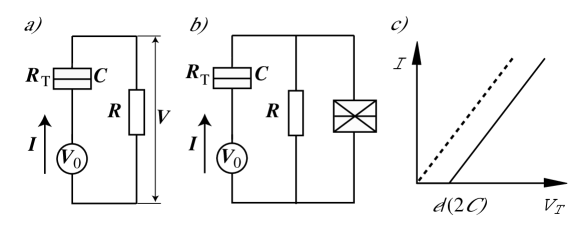
We consider the simplest circuit, which is standard for studies of shot noise in tunnel junctions: a tunnel junction of resistance $R_{T}$ and of capacitance $C$ biased from an ideal voltage source $V_{0}$ via a resistance $R$ (called shunt) in series (Fig. 1a). The voltage across the junction is $V_{T}=V_{0}-V$ where $V=IR$ is the voltage over the shunt resistor and $I=V_{0}/(R_{T}+R)$ is the current through the junction. A basic parameter for our analysis is the ratio $\alpha=R/R_{T}$. If $\alpha\ll 1$ the circuit corresponds to an ideal voltage bias $V_{0}\approx V_{T}$, whereas if $\alpha\gg 1$ this is the case of ideal current bias.

The standard method of noise spectroscopy is to measure voltage $V$ at the shunt OddE ; Rez . On the other hand, a Josephson junction added parallel to the shunt (Fig. 1b) may probe the phase difference fluctuations at the shunt ours ; TNP . We assume that the both resistances, $R_{T}$ and $R$, clearly exceed the quantum resistance $R_{K}=h/e^{2}$. According to the orthodox theory AL at $T=0$, in this limit the average rate of tunneling through the junction at $V_{T}>e/2C$ is $(V_{T}-e/2C)/eR_{T}$. The $IV$ curve for an ideal voltage bias ($V_{T}\approx V_{0}$) is shown in Fig. 1c. The junction is Coulomb blockaded as far as the voltage $V_{T}$ does not exceed the Coulomb voltage offset $e/2C$.

Figure 1: Electric circuit. a) Normal tunnel junction voltage-biased through the shunt resistance $R$. b) Parallel to the shunt there is a Josephson junction, which probes the phase difference at the shunt. c) The $IV$ curve of the normal junction in the limit of ideal voltage bias.

III Full statistics for ideal voltage bias

There is a straightforward procedure to find the full statistics in the limit of ideal voltage bias exactly ours ; TNP . Because of the constant voltage at the junction the probability of tunneling is also constant and the full counting statistics is given by the Poissonian distribution. The generating function, which yields all moments and cumulants, is

$$F_{c}(\lambda,t)=\sum_{n}e^{\lambda n}P_{n}(t)=e^{(V_{T}t/eR_{T})(e^{\lambda}-1)}=e^{(It/e)(e^{\lambda}-1)}~{},$$ (1)

where $P_{n}(t)=e^{-\bar{n}}\bar{n}^{n}/n!$ is the Poissonian distribution, $n$ is the number of tunneling events during the time interval $t$. The average number of events is determined by the current: $\bar{n}=It/e$.

Though in the limit of ideal voltage bias the voltage at the junction $V_{T}\approx V_{0}$ practically does not vary, the small voltage $V\ll V_{0}$ at the shunt strongly fluctuates. In order to find the statistics of voltage $V$ let us consider a sequence of $N$ tunneling events at random moments of time $t_{j}$ ($j=1,2,...N$), which may occur during the long time interval $T$. Time $T$ is connected with $N$ via the relation $N=IT/e$. Any tunneling produces the voltage pulse at the shunt, so the voltage varies in time as

$$V(t)=\sum_{j=1}^{N}{e\over C}e^{-(t-t_{j})/\tau}\Theta(t-t_{j})~{},$$ (2)

where $\tau=RC$ and $\Theta(t)$ is the step function. Then one can find the generating function for the voltage distribution averaging over random moments of time $t_{j}$:

$$F_{v}(\nu)=\left\langle e^{\nu v}\right\rangle=\left\langle e^{\nu\sum_{j}e^{-(t-t_{j})/\tau}}\right\rangle=\prod_{j=1}^{N}\int_{0}^{T}{dt_{j}\over T}e^{\nu e^{-(t-t_{j})/\tau}\Theta(t-t_{j})}$$

$$=\left(1+{\Phi_{v}(\nu)\over T}\right)^{N}=e^{\Phi(\nu)I/e}~{},$$ (3)

where the dimensionless voltage $v=VC/e$ was introduced,

$$\Phi_{v}(\nu)=\int_{0}^{\infty}dt\left(e^{\nu e^{-t/\tau}}-1\right)=\tau[\mbox{E}_{1}(-\nu)-\gamma-\ln(-\nu)]$$ (4)

is the contribution of a single tunneling event, $\gamma$ is Euler’s constant, and $E_{1}(z)=\int_{z}^{\infty}(e^{z}-1)dz/z$ is the exponential integral.

Let us consider the random phase variation, which follows from Eq. (2) and the Josephson relation $d\varphi/dt=eV/\hbar$:

$$\varphi(t)=\sum_{j=1}^{N}r\left[1-e^{-(t-t_{j})/\tau}\right]\Theta(t-t_{j})~{},$$ (5)

where $r=2\pi R/R_{K}$. Our goal is to find the full statistics for the phase difference $\Delta\varphi(t)=\varphi(t+t_{0})-\varphi(t_{0})=\sum_{j}\delta\varphi_{j}$ during a fixed time interval $t$, where the contribution from the tunneling at the moment $t_{j}$ is

$$\delta\varphi_{j}=r\left[1-e^{-(t+t_{0}-t_{j})/\tau}\right]\Theta(t+t_{0}-t_{j})-r\left[1-e^{-(t_{0}-t_{j})/\tau}\right]\Theta(t_{0}-t_{j})~{}.$$ (6)

Similar to the voltage statistics one should find the generating function for the phase difference, which does not depend on $t_{0}$ after averaging:

$$F_{\varphi}(\xi,t)=\left\langle e^{\xi\Delta\phi(t)}\right\rangle=\prod_{j=1}^{N}\int_{0}^{T}{dt_{j}\over T}e^{\xi\delta\varphi_{j}/r}=\left(1+{\Phi_{\varphi}(\xi)\over T}\right)^{N}=e^{\Phi_{\varphi}(\xi,t)I/e}~{},$$ (7)

where $\phi=\varphi/r$ is the rescaled phase and

$$\Phi_{\varphi}(\xi,t)=-t-\tau\left\{e^{\xi}\left[E_{1}(\xi)-E_{1}\left(\xi e^{-t/\tau}\right)\right]+E_{1}\left[-\xi\left(1-e^{-t/\tau}\right)\right]\right.$$

$$\left.+\gamma+\ln\left[-\xi\left(1-e^{-t/\tau}\right)\right]\right\}~{}.$$ (8)

We have introduced the rescaled phase since after this, statistics of phase at long times is identical to counting statistics (see below). Note that at $\xi=ir$ the generating function $F_{\varphi}(\xi,t)$ yields the phase correlator $\langle e^{i\varphi(t)-i\varphi(0)}\rangle$, which determines the current through the normal tunnel junction in the $P(E)$ theory, whereas at $\xi=2ir$ this yields the phase correlator for the Cooper pairs in the Josephson junction ours ; TNP . At long times $t\gg\tau$ the phase statistics becomes identical to the counting statistics (apart from the scaling factor $r$):

$$F_{\varphi}(\xi,t)=e^{(It/e)(e^{\xi}-1)}~{}.$$ (9)

This is equal to $F_{c}(\lambda,t)$, Eq. (1), with $\lambda=\xi$. On the other hand at short times $t\ll\tau$ the voltage does not vary essentially during the time $t$, and the phase statistics should be identical to the voltage statistics. Indeed, at $t\ll\tau$ Eq. (7) yields the voltage generating function $F_{v}(\nu)$, Eq. (3), with $\nu=\xi t/\tau$.

IV Full voltage statistics from master equation

In order to find the full voltage statistics for an arbitrary bias we use the master equation for the voltage probability density $P(V,t)$:

$${\partial P(V,t)\over\partial t}-{1\over RC}{\partial\over\partial V}[VP(V,t)]$$

$$+{1\over eR_{T}}\left[\left(V_{T}-{e\over 2C}\right)P(V,t)-\left(V_{T}+{e\over 2C}\right)P\left(V-{e\over C},t\right)\right]=0~{}.$$ (10)

This equation directly follows from the master equation in Ref. AL, in the limit $T\to 0$ when tunneling can occur only in one direction. Our analysis addresses the case of high currents when the voltage $V_{T}$ at the junction always exceeds the Coulomb gap $e/2C$. We remind that we consider the high-impedance circuit when the resistances $R$ and $R_{T}$ exceed the quantum resistance.

The equation for the generating function ($v=VC/e$),

$$F_{v}(\nu)=\int e^{\nu v}P(V)dV~{},$$ (11)

is obtained by integration of the master equation over the whole interval of relevant voltages:

$${\partial F_{v}(\nu)\over\partial t}+{\nu\over RC}{\partial F_{v}(\nu)\over\partial\nu}+{e^{\nu}-1\over eR_{T}}\left[{e\over C}{\partial F_{v}(\nu)\over\partial\nu}-\left(V_{0}-{e\over 2C}\right)F_{v}(\nu)\right]=0~{}.$$ (12)

In terms of the dimensionless time $\tilde{t}=t/RC$ and the dimensionless voltage $v_{0}=VC/e$, the equation becomes:

$${\partial F_{v}(\nu)\over\partial\tilde{t}}+[\nu+\alpha(e^{\nu}-1)]{\partial F_{v}(\nu)\over\partial\nu}-\alpha(e^{\nu}-1)\left(v_{0}-{1\over 2}\right)F_{v}(\nu)=0~{}.$$ (13)

In the stationary case this is an ordinary differential equation with respect to $\nu$, which has the following solution:

$$F_{v}(\nu)=\exp\left[\left(v_{0}-{1\over 2}\right)\int_{0}^{\nu}\frac{\alpha(e^{z}-1)}{z+\alpha(e^{z}-1)}dz\right]~{}.$$ (14)

The solution satisfies the natural boundary condition that $F_{v}(\nu)=1$ at $\nu=0$. According to Eq. (11) this provides a proper normalization of the probability density.

The limit $\alpha=R/R_{K}\to 0$ corresponds to the ideal-bias case when the generating functions given by Eqs. (3) and (14) are identical keeping in mind that the current is $I=(V_{0}-e/2C)/(R_{T}+R)$. In the general case of arbitrary $\alpha$, the first three cumulants for the voltage at the shunt are:

$$\langle\langle V\rangle\rangle={e\over C}{d\ln F_{v}(\nu)\over d\nu}=IR~{},$$

$$\langle\langle V^{2}\rangle\rangle={e^{2}\over C^{2}}{d^{2}\ln F_{v}(\nu)\over d\nu^{2}}={IR\over 2(1+\alpha)}{e\over C}~{},$$

$$\langle\langle V^{3}\rangle\rangle={e^{3}\over C^{3}}{d^{3}\ln F_{v}(\nu^{3})\over d\nu^{3}}={IR(2-\alpha)\over 6(1+\alpha)^{2}}{e^{2}\over C^{2}}~{}.$$ (15)

The first cumulant is simply the average voltage at the shunt. The third cumulant (skewness) of the voltage distribution changes sign at $\alpha=1/2$. The width of the distribution is determined by the smallest from the two voltages: the shunt voltage $IR$ for the ideal voltage bias ($\alpha\to 0$), or the junction voltage $IR_{T}$ for the ideal current bias ($\alpha\to\infty$).

V Full phase statistics

In order to find the full phase statistics one should consider the master equation for voltage and phase. We introduce the probability density $P(V,\varphi,t)$ for the shunt voltage $V$ and the corresponding phase $\varphi(t)=(e/\hbar)\int^{t}V(t^{\prime})dt^{\prime}$. The master equation is:

$${\partial P(V,\varphi,t)\over\partial t}+{eV\over\hbar}{\partial P(V,\varphi,t)\over\partial\varphi}-{1\over RC}{\partial\over\partial V}[VP(V,\varphi,t)]$$

$$+{1\over eR_{T}}\left[\left(V_{T}-{e\over 2C}\right)P(V,\varphi,t)-\left(V_{T}+{e\over 2C}\right)P\left(V-{e\over C},\varphi,t\right)\right]=0~{}.$$ (16)

The full statistics of voltage and phase is determined by the generating function for the united phase+voltage probability distribution:

$$F_{v\varphi}(\xi,\nu,t)=\int e^{\xi\phi+\nu v}P(V,\varphi,t)d\varphi\,dV~{},$$ (17)

where $\phi=\varphi/r$ is the rescaled phase and $v=VC/e$ is the rescaled voltage. The master equation yields the following equation for the generating function

$${\partial F_{v\varphi}(\xi,\nu,\tilde{t})\over\partial\tilde{t}}+\left[\nu-\xi+\alpha(e^{\nu}-1)\right]{\partial F_{v\varphi}(\xi,\nu,\tilde{t})\over\partial\xi}-\alpha(e^{\nu}-1)\left(v_{0}-{1\over 2}\right)F_{v\varphi}(\xi,\nu,\tilde{t})=0~{}.$$ (18)

Here we use dimensionless time $\tilde{t}=t/RC$. There is a well known analogy of the phase with a coordinate of a diffusing particle and of the voltage with a particle velocity. Correspondingly, the phase distribution can never be stationary and permanently expands. Thus the generating function is always time-dependent. Performing the Laplace transformation,

$$F_{v\varphi}(\xi,\nu,s)=\int_{0}^{\infty}e^{-s\tilde{t}}F_{v\varphi}(\xi,\nu,\tilde{t})d\tilde{t}~{},$$ (19)

the equation for the generating function becomes

$$sF_{v\varphi}(\xi,\nu,s)+\left[\nu-\xi+\alpha(e^{\nu}-1)\right]{dF_{v\varphi}(\xi,\nu,s)\over d\xi}-\alpha(e^{\nu}-1)\left(v_{0}-{1\over 2}\right)F_{v\varphi}(\xi,\nu,s)$$

$$=F_{v\varphi}(\xi,\nu,t)|_{t=0}~{},$$ (20)

where $F_{v\varphi}(\xi,\nu,t)|_{t=0}$ is the initial value of the generating function. The solution of this nonuniform differential equation is

$$F_{v\varphi}(\xi,\nu,s)=F_{0}(\xi,\nu,s)\int_{\xi_{1}+\delta}^{\nu}{F_{v\varphi}(\xi,x,t)|_{t=0}\over[-\xi+x+\alpha(e^{x}-1)]F_{0}(\xi,x,s)}dx~{},$$ (21)

where $\xi_{1}$ is a zero of the denominator in the integrand function,

$$-\xi+\xi_{1}+\alpha(e^{\xi_{1}}-1)=0~{},$$ (22)

and

$$F_{0}(\xi,\nu,s)=\exp\left[\int_{\xi_{1}+\delta}^{\nu}{-s+\left(v_{0}-{1\over 2}\right)\alpha(e^{x}-1)\over-\xi+x+\alpha(e^{x}-1)}dx\right]$$ (23)

is the solution of the uniform equation when the right-hand part of Eq. (20) vanishes. In order to cut divergence at the pole at $x\to\xi_{1}$, an infinitely small constant $\delta$ was introduced. In final expressions this divergence is canceled and the limit $\delta\to 0$ yields convergent results. One can check that the solution Eq. (21) satisfies the boundary condition $F_{v\varphi}(\xi,\nu,t)=1$ at $\xi=\nu=0$, which provides a proper normalization of the probability density. The Laplace transform of this condition is $F_{v\varphi}(\xi,\nu,s)=1/s$ at $\xi=\nu=0$. In order to obtain the full phase statistics from the solution Eq. (21) one should choose the initial condition that

$$F_{v\varphi}(\xi,\nu,t)|_{t=0}=F_{v}(\nu)~{},$$ (24)

where $F_{v}(\nu)$ is the generating function for the stationary shunt voltage distribution given by Eq. (14). Independence of this function on $\xi$ means that we fixed the phase $\varphi=0$ at the initial moment of time $t=0$. Finally the full phase statistics after averaging over the voltage is given by:

$$F_{\varphi}(\xi,s)=F_{v\varphi}(\xi,0,s)=F_{0}(\xi,0,s)\int_{\xi_{1}+\delta}^{0}{F_{v}(x)\over[-\xi+x+\alpha(e^{x}-1)]F_{0}(\xi,x,s)}dx~{}.$$ (25)

Taking derivatives with respect to the variable $\xi$ conjugate to the phase difference one may obtain any moment or cumulant for the phase-difference probability. But even for the second or the third cumulant taking derivatives is a tiresome procedure in general. So we restrict the further analysis with some limiting cases.

Long-time limit

This case was also analyzed quantum-mechanically KNB . We shall see that our general classical analysis completely agrees with it.

In the case of the long-time asymptotics the most important contribution to the integral in (25) comes from the close vicinity of the pole determined by Eq. (22). The solution of the uniform equation, Eq. (23), can be also reduced to the contribution of the pole, and

$$F_{0}(\xi,\nu,s)\approx\exp\left[\int_{\xi_{1}+\delta}^{\nu}{-s+s_{0}\over-\xi+x+\alpha(e^{x}-1)}dx\right]\approx\left({\delta\over\nu-\xi_{1}}\right)^{(s_{0}-s)/(1+\alpha)}~{},$$ (26)

where

$$s_{0}=\left(v_{0}-{1\over 2}\right)\alpha(e^{\xi_{1}}-1)~{}.$$ (27)

For long-time asymptotics the initial condition for the generating function is not essential, and one can assume for simplicity that $F_{v\varphi}(\xi,x,t)|_{t=0}=F_{v}(x)=1$ in Eq. (25). This means that at $t=0$ the voltage and phase difference at the shunt are zero. Finally the Laplace transform of the generating function for phase probability is approximated at long times with

$$F_{\varphi}(\xi,s)\approx{1\over s-s_{0}}~{}.$$ (28)

After the inverse Laplace transformation the generating function in the time presentation is

$$F_{\varphi}(\xi,t)\approx e^{s_{0}\tilde{t}}~{}.$$ (29)

This fully agrees with the result obtained by Kindermann et al. KNB from the quantum-mechanical analysis. This is a manifestation of a simple law, which Kindermann et al. have formulated for the full statistics of two devices connected in series with the ideal voltage source. If the full statistics (either counting statistics or phase statistics) for any of two devices connected directly to the voltage source without another device are $F_{1}(\xi_{1})$ or $F_{2}(\xi_{2})$ respectively, then for the two devices connected together the full statistics is $F(\xi)=F_{1}(\xi_{1})=F_{2}(\xi_{2})$ at the condition that $\xi=\xi_{1}+\xi_{2}$. In our case, the two devices are a normal tunnel junction and a macroscopic resistor (shunt). Then $F_{1}(\xi_{1})=e^{(It/e)(e^{\xi_{1}}-1)}$ follows from the phase statistics of the junction at the ideal voltage bias, Eq. (9), whereas $F_{2}(\xi_{2})=e^{(It)\xi_{2}/e}$ corresponds to a macroscopic resistor (shunt) under fixed voltage bias $IR$. Equation (22) is identical to the equation $F_{1}(\xi_{1})=F_{2}(\xi-\xi_{1})$.

The generating function Eq. (29) yields the following first 4 cumulants:

$$\langle\langle\varphi\rangle\rangle=r{d\ln F_{\varphi}\over d\xi}=r{ds_{0}\over d\xi}\tilde{t}=r{ds_{0}\over d\xi_{1}}{d\xi_{1}\over d\xi}\tilde{t}=r\left(v_{0}-{1\over 2}\right)\tilde{t}{\alpha\over 1+\alpha}=r{It\over e}~{},$$ (30)

$$\langle\langle\varphi^{2}\rangle\rangle=r^{2}{d^{2}\ln F_{\varphi}\over d\xi^{2}}=r^{2}\left(v_{0}-{1\over 2}\right)\tilde{t}{\alpha\over(1+\alpha)^{3}}=r^{2}{It\over e}{1\over(1+\alpha)^{2}}~{},$$ (31)

$$\langle\langle\varphi^{3}\rangle\rangle=r^{3}{d^{3}\ln F_{\varphi}\over d\xi^{3}}=r^{3}\left(v_{0}-{1\over 2}\right)\tilde{t}{\alpha(1-2\alpha)\over(1+\alpha)^{5}}=r^{3}{It\over e}{1-2\alpha\over(1+\alpha)^{4}}~{},$$ (32)

$$\langle\langle\varphi^{4}\rangle\rangle=r^{4}{d^{4}\ln F_{\varphi}\over d\xi^{4}}=r^{4}\left(v_{0}-{1\over 2}\right)\tilde{t}{\alpha(1-8\alpha+6\alpha^{2})\over(1+\alpha)^{7}}=r^{4}{It\over e}{1-8\alpha+6\alpha^{2}\over(1+\alpha)^{6}}~{}.$$ (33)

Kindermann et al. KNB have shown that in the limit of ideal current bias ($\alpha\gg 1$) the statistics of the phase at a contact of arbitrary transparency corresponds to the Pascal distribution Spi . If the contact transparency is very low (the case of tunnel junction) the Pascal distribution is reduced to the chi-square distribution. One can check that this fully agrees with our analysis, and the found full phase statistics corresponds to the chi-square distribution for phase probability.

Short-time limit

The full phase statistics for short time intervals directly follows from a plausible assumption that the voltage does not vary during the observation time. This means that the generating function $F_{\varphi}(\xi)$ for the phase is equal to the generating function $F_{v}(\nu)$ for the voltage, Eq. (14), with $\nu=\xi t/\tau$ as directly proved for an ideal voltage bias in Sec. III.

Our analysis shows that the crossover between the long-time and the short-time behavior is governed by the relaxation time $\tilde{\tau}=CRR_{T}/(R_{T}+R)$. This time is different from the relaxation time $\tau=RC$, which characterizes the electron transport in the circuit between tunneling events. The two relaxation times coincide only in the ideal-voltage-bias limit.

VI Counting statistics

In order to find the full counting statistics we introduce the density $P_{n}(V,t)$ of probability that during the time interval $t$ $n$ electrons tunneled through the junction and that in the end of the interval the voltage at the shunt is $V$. The master equation for this probability is

$${\partial P_{n}(V,t)\over\partial t}-{1\over RC}{d\over dV}[VP_{n}(V,t)]$$

$$+{1\over eR_{T}}\left[\left(V_{T}-{e\over 2C}\right)P_{n}(V,t)-\left(V_{T}+{e\over 2C}\right)P_{n-1}\left(V-{e\over C},t\right)\right]=0~{}.$$ (34)

Let us introduce the generating function:

$$F_{cv}(\lambda,\nu,t)=\sum_{n}e^{\lambda n}\int e^{\nu v}P_{n}(V,t)dV~{}.$$ (35)

The Laplace transform of the equation for the generating function is (the dimensionless time variable $\tilde{t}=t/RC$ was used):

$$sF_{cv}(\lambda,\nu,s)+{dF_{cv}(\lambda,\nu,s)\over d\nu}\left[\nu+\alpha(e^{\lambda+\nu}-1)\right]-v_{0}\alpha(e^{\lambda+\nu}-1)F_{cv}(\lambda,\nu,s)$$

$$=F_{cv}(\lambda,\nu,t)|_{t=0}~{}.$$ (36)

The left-hand side of this equation is identical to the left-hand side of Eq. (20) after transformation $\xi=\lambda+\nu$. The full counting statistics corresponds to the limit $\nu\to 0$. Eventually the generating function can be easily obtained from Eq. (25) for the full phase statistics:

$$F_{c}(\lambda,s)=F_{0}(\lambda,0,s)\int_{\xi_{1}+\delta}^{0}{F_{v\varphi}(\lambda+x,x,t)|_{t=0}\over[-\lambda+x+\alpha(e^{x}-1)]F_{0}(\lambda,x,s)}dx~{}.$$ (37)

Long times

The only difference between the phase statistics and the full counting statistics appears in the initial boundary condition. Since for the long-time asymptotic the initial boundary condition is not essential, in this limit the cumulants for the full counting statistics can be obtained from those for the full phase statistics [Eqs. (30-31)] by simple rescaling. Namely, the relation between two types of cumulants is $\langle\langle n^{k}\rangle\rangle=\langle\langle\phi^{k}\rangle\rangle=\langle\langle\varphi^{k}\rangle\rangle/r^{k}$. This relation was derived by Kindermann et al. KNB , but it was approximate in their quantum-mechanical analysis. In our purely classical approach this relation is exact.

Short times

In analogy with the short-time limit ($t\ll\tilde{\tau}$) of the phase statistics we use the fact that the voltage does not vary essentially during the time $t$. If one considers a subensemble of realizations, which correspond to some fixed voltage $V_{T}$ at the junction during the time interval $t$, the distribution of numbers of tunneling events is Poissonian and the generating function is given by Eq. (1). But one should take into account that the voltage $V_{T}$ at the junction fluctuates. Thus one should average over $V_{T}=V_{0}-V$, and the generating function is given by

$$F_{c}(\lambda,t)=\int e^{(V_{T}t/eR_{T})(e^{\lambda}-1)}P(V_{T})dV_{T}=\int e^{[(V_{0}-V)t/eR_{T}(e^{\lambda}-1)}P(V)dV~{}.$$ (38)

One can see that the generating function for the counting statistics is directly connected with the generating function for the voltage, Eq. (11):

$$F_{c}(\lambda,t)=e^{(V_{0})t/eR_{T}(e^{\lambda}-1)}F_{v}(\tilde{\nu})~{},$$ (39)

where

$$\tilde{\nu}=-{t\over R_{T}C}(e^{\lambda}-1)~{}.$$ (40)

This allows to obtain expressions for any cumulant of the full counting statistics using the expressions for voltage cumulants, Eq. (15). The first three of them are:

$$\langle\langle n\rangle\rangle={d\ln F_{c}\over d\lambda}={V_{0}t\over eR_{T}}+{d\ln F_{v}\over d\tilde{\nu}}{d\tilde{\nu}\over d\lambda}$$ (41)

$$={V_{0}t\over eR_{T}}-\langle\langle V\rangle\rangle{C\over e}{t\over R_{T}C}={It\over e}~{},$$ (42)

$$\langle\langle n^{2}\rangle\rangle={d^{2}\ln F_{c}\over d\lambda^{2}}={V_{0}t\over eR_{T}}+{d\ln F_{v}\over d\tilde{\nu}}{d^{2}\tilde{\nu}\over d\lambda^{2}}+{d^{2}\ln F_{v}\over d\tilde{\nu}^{2}}\left({d\tilde{\nu}\over d\lambda}\right)^{2}={V_{0}t\over eR_{T}}-\langle\langle V\rangle\rangle{C\over e}{t\over R_{T}C}$$

$$+\langle\langle V^{2}\rangle\rangle{C^{2}\over e^{2}}\left({t\over R_{T}C}\right)^{2}={It\over e}\left[1+{t\over\tilde{\tau}}{\alpha^{2}\over 2(1+\alpha)^{2}}\right]~{},$$ (43)

$$\langle\langle n^{3}\rangle\rangle={d^{3}\ln F_{c}\over d\lambda^{3}}={V_{0}t\over eR_{T}}e^{\lambda}+{d\ln F_{v}\over d\tilde{\nu}}{d^{3}\tilde{\nu}\over d\lambda^{3}}+3{d^{2}\ln F_{v}\over d\tilde{\nu}^{2}}{d^{2}\tilde{\nu}\over d\lambda^{2}}{d\tilde{\nu}\over d\lambda}+{d^{3}\ln F_{v}\over d\tilde{\nu}^{3}}\left({d\tilde{\nu}\over d\lambda}\right)^{3}\to{It\over e}$$

$$+3\langle\langle V^{2}\rangle\rangle{C^{2}\over e^{2}}\left({t\over R_{T}C}\right)^{2}-\langle\langle V^{3}\rangle\rangle{C^{3}\over e^{3}}\left({t\over R_{T}C}\right)^{3}$$

$$={It\over e}\left[1+{t\over\tilde{\tau}}{3\alpha^{2}\over 2(1+\alpha)^{2}}-\left({t\over\tilde{\tau}}\right)^{2}{\alpha^{3}(2-\alpha)\over 6(1+\alpha)^{4}}\right]~{}.$$ (44)

These expressions demonstrate that at short times $t\ll\tilde{\tau}=CRR_{T}/(R_{T}+R)$ the counting statistics becomes Poissonian even in the limit of current bias $\alpha\to\infty$. Thus for short times the circuit (environment) effects are not so essential as for long times. It is worthwhile to note that “short” times $t\ll\tilde{\tau}$ in reality are not necessarily short compared with the average time $e/I$ between tunneling events since we consider the case of high currents $I$, and very many electrons may tunnel during the “short” time $t\ll\tilde{\tau}$.

VII Numerical simulation

In our computational model, the time dependence of charge $Q(t)=CV_{T}(t)$ on the junction with capacitance $C$ is obtained by integrating the equation

$$\frac{dQ}{dt}=\frac{V_{0}-Q/C}{R}-\left(\frac{dQ}{dt}\right)_{T},$$ (45)

where the first term on the right represents charge relaxation through the shunt resistor $R$, and the latter term represents tunneling current in the tunnel junction. According to Sec. II at $V_{T}>e/2C$ the average tunneling rate $\langle dQ_{I}/dt_{T}\rangle$ is $(Q/e-1/2)/RC$. Employing standard Monte-Carlo methods, this average rate is used to generate tunneling events, which are considered to take place instantaneously on the time scales of other processes. A ready-made, Mersenne-Twisters-type random number generator Mersenne was employed in our Fortran code.

The simulation was performed using parameter values close to standard mesoscopic tunnel junctions, namely $R_{T}=10$ k$\Omega$ and $C=1$ fF which corresponds to a Coulomb voltage of $e/2C\sim 0.1$ mV. We used $V_{0}=5$ mV for the bias voltage, while the length of the time record was typically set to 1 ns. With these values our time trace displayed altogether a few hundred tunneling events. The relaxation rate $\tilde{\tau}=CRR_{T}/(R_{T}+R)$ normally does not exceed 10 ps, and our simulation is basically in the long time limit discussed in Secs. V and VI. The time step in the integration was $\Delta t=10^{-14}-10^{-13}$ s. The simulation was initialized for 50000 iterations before starting the calculation of the actual time traces. For making distributions, the calculation was repeated for $5-10\cdot 10^{5}$ times using the previous simulation as an initialization for the next one.

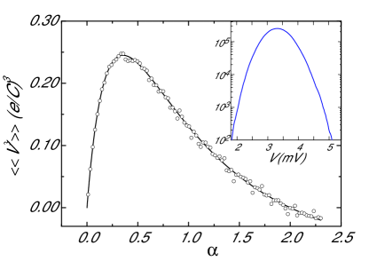
Fig. 2 characterizes the skewness of the distribution of the voltage $V$ over the shunt resistor obtained in our simulations. The inset displays the logarithm of a voltage distribution $\ln P(V)$, calculated at $\alpha=0.5$. The asymmetry is clearly visible in the wings of the $\ln P(V)$-curve. The solid curve depicts the theoretical curve for $\langle\langle V^{3}\rangle\rangle$ obtained from Eq. (15). The master equation approach is seen to agree with the Monte-Carlo simulation within the scatter of the data points.

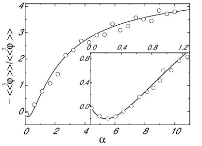
Phase $\varphi(t)$ was calculated from the simulated voltage trace by numerically evaluating $\int dtV(t)$ using a 3-point Simpson rule. Fig. 3 displays the result for the ratio $\langle\langle\varphi^{3}\rangle\rangle/\langle\langle\varphi^{2}\rangle\rangle$; we have chosen this ratio as both the nominator and the denominator are proportional to $I$, eliminating the bias dependence off from it. The behavior at small values of $\alpha$ is illustrated in the inset in more detail. The simulated data are seen to display a change of sign in a similar manner as in the theory at $\alpha=0.5$. Notice that the functional dependence here coincides with the current fluctuation results in the low-frequency limit KNB .

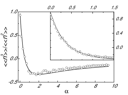
Fig. 4 illustrates the ratio of the skewness to the variance for the counting statistics as a function of the parameter $\alpha$ in the long-time limit, i.e. when the length of the time trace exceeds the relaxation time $\tilde{\tau}=CRR_{T}/(R_{T}+R)$. In general, we find a good agreement between our Monte-Carlo simulation and the ratio calculated from Eqs. (31) and (32) with help of the relation $\langle\langle n^{k}\rangle\rangle=\langle\langle\varphi^{k}\rangle\rangle/r^{k}$, except for a small offset at $\alpha>2$. The inset magnifies the results at $\alpha<1.5$: the data on $\langle\langle n^{3}\rangle\rangle/\langle\langle n^{2}\rangle\rangle$ is seen to approach the Poisson result $\langle\langle n^{3}\rangle\rangle/\langle\langle n^{2}\rangle\rangle=1$ as expected when $\alpha\rightarrow 0$.

Figure 2: Skewness of the voltage distribution over the shunt resistor as a function of $\alpha=R/R_{T}$. The solid curve is calculated using Eq. (15). The inset displays the probability distribution $P(V)$ for voltage at $\alpha=0.5$ in arbitrary units.

Figure 3: Illustration of phase statistics over the shunt resistor in terms of the ratio $\langle\langle\varphi^{3}\rangle\rangle/\langle\langle\varphi^{2}\rangle\rangle$. The solid curve is calculated using Eqs. (31) and (32). The inset displays a magnification of the initial part of the data.

Figure 4: Ratio of the second and the third cumulants of the counting statistics distribution. The solid curve is calculated using Eqs. (31) and (32) and the relation $\langle\langle n^{k}\rangle\rangle=\langle\langle\varphi^{k}\rangle\rangle/r^{k}$. The inset displays a magnification of the initial part of the data.

VIII Conclusions

Our classical approach based on the master equation provides the full statistics of electron transport through a normal junction in a high-impedance circuit. In addition to the full counting statistics, the statistics of voltage and phase at the shunt resistor was found. The analysis is valid for any time interval of observation. The results are in full agreement with the results of the quantum-mechanical analysis performed in the long-time limit KNB . In particular, the crossover of full counting statistics from the Poissonian in the voltage-biased limit to the chi-square distribution in the current-biased case was obtained. The identity of counting statistics and phase statistics, which was found as an approximate result of the quantum-mechanical analysis KNB , was proven to be exact within classical approach. Our analysis shows that strong environment (circuit) effects on counting statistics become much weaker at short time scales (high frequencies). We have performed numerical simulations using Monte-Carlo methods, which fully agree with our analytical results.

References

• (1) W. Schottky, Annalen der Physik 57, 541 (1918).
• (2) Ya.M. Blanter and M. BΓΌttiker, Phys. Rep. 336, 1 (2000).
• (3) L.S. Levitov and G.B. Lesovik, Pis’ma Zh. Eksp. Teor. Fiz. 58, 225 (1993) [JETP Lett. 58, 230 (1993)].
• (4) M. Kindermann, Yu.V. Nazarov, and C.W. J. Beenakker, Phys. Rev. Lett. 90, 246805 (2003).
• (5) B. Reulet, J. Senzier, and D.E. Prober, Phys. Rev. Lett. 91, 196601 (2003).
• (6) Yu. Bomze, G. Gershon, D. Shovkun, L.S. Levitov, and M. Reznikov, cond-mat/0504382.
• (7) J. Delahaye, R. Lindell, M.S. SillanpÀÀ, M.A. Paalanen, E.B. Sonin, and P.J. Hakonen, cond-mat/0209076 (unpublished); R. Lindell, J. Delahaye, M.A. SillanpÀÀ, T.T. HeikkilΓ€, E.B. Sonin, and P.J. Hakonen, Phys. Rev. Lett. 93, 197002 (2004); E. B. Sonin, Phys. Rev. B 70, 140506(R) (2004).
• (8) E.B. Sonin, cond-mat/0505424.
• (9) J. Tobiska and Yu.V. Nazarov, Phys.Rev. Lett. 93, 106801 (2004).
• (10) J.P. Pekola, Phys.Rev. Lett. 93, 206601 (2004); J.P. Pekola, T.E. Nieminen, M. Meschke, J.M. Kivioja, A.O. Niskanen, and J.J. Vartiainen, cond-mat/0502446.
• (11) K.E. Nagaev, Phys. Rev. 66, 075334 (2002); cond-mat/0512246.
• (12) D.V. Averin and K.K. Likharev, in: Mesoscopic Phenomena in Solids, ed. B.L. Altshuler, P.A. Lee, and R.A. Webb, (Elsevier, 1991), p. 173.
• (13) D.A. Bagrets and Yu.V. Nazarov, Phys. Rev. B 67, 085316 (2003).
• (14) M.R. Spiegel, Theory and problems of probability and statistics, (McGraw Hill, N.Y., 1975)., p. 115.
• (15) Matsumoto and T. Nishimura, ACM Trans. on Modeling and Computer Simulation 8, 3 (1998).