Equations of motion approach to decoherence and current noise in ballistic interferometers coupled to a quantum bath

Abstract

We present a technique for treating many particles moving inside a ballistic interferometer, under the influence of a quantum-mechanical environment (phonons, photons, Nyquist noise etc.). Our approach is based on solving the coupled Heisenberg equations of motion of the many-particle system and the bath and is inspired by the quantum Langevin method known for the Caldeira Leggett model. It allows to study decoherence and the influence of the bath on other properties of the interferometer. As a first application, we treat a fermionic Mach-Zehnder interferometer. In particular, we discuss the dephasing rate and present full analytical expressions for the leading corrections to the current noise, brought about by the coupling to the quantum bath.

I Introduction

Decoherence, the destruction of quantum-mechanical phase coherence by a fluctuating environment, plays an important role, ranging from fundamental questions such as the quantum-classical correspondence to potential applications (like quantum information). For most of the recent two decades, the focus of research has been on quantum-dissipative systems with few degrees of freedom: the most prominent examples are the single particle (e.g. Caldeira-Leggett model callegg ; Weiss ) or a single two-level system (spin-boson model) and other impurity models (e.g. the Kondo model in transport through quantum dots). However, such a description is no longer adequate when it comes to transport interference effects both in disordered systems (weak localization, universal conductance fluctuations) or man-made interference devices (Aharonov-Bohm rings, double quantum dot interferometers, atom chip interference setups etc.). In those cases, we are dealing with a many-particle system. As long as this is coupled to classical noise, we can still use the single particle picture. Both the technical effort and the physical ideas expand considerably when going over to a full quantum bath. Up to now, there have been comparatively few treatments of quantum-dissipative many-particle systems (for examples see OpenLuttLiquids ; aleinerwhichpath ; ABring ; DDot ; FlorianDima and references therein).

In this article, we describe an equations of motion approach for ballistic interferometers coupled to a quantum bath (Fig. 1). It is physically transparent, more efficient than generic methods (like Keldysh diagrams) and straightforwardly keeps important physics, such as the effects of Pauli blocking in fermionic systems. It may be applied to describe decoherence (or dephasing; we use the terms interchangeably) and, in general, to calculate the current noise and other higher-order correlators of the particle field.

We have already introduced this method in a recent short articleEPL , and applied it to the electronic Mach-Zehnder interferometer realized at the Weizmann instituteHeiblumEtAl , discussing the loss of visibility in the current interference pattern and (briefly) the effects on the current noise. The purpose of the present paper is four-fold: (i) to relate our many-particle method to the Quantum Langevin equation as it is known for a single particle in the context of the Caldeira-Leggett model (Sec. II.1), (ii) to provide more details of the method and on how to evaluate the resulting expressions using perturbation theory (Sec. IV.3), (iii) to derive and present full analytical expressions for the leading correction to the current noise of a MZ setup coupled to a quantum bath (Sec. IV.4), and (iv) to add to our previous brief discussion of the current noise (Sec. IV.5).

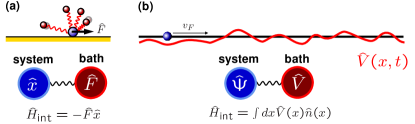
Figure 1: (a) The Caldeira-Leggett model (single particle and oscillator bath) and (b) a ballistic many-particle system subject to a quantum noise potential $\hat{V}(x,t)$.

II Equations of motion approach to decoherence in ballistic interferometers

II.1 Brief reminder of the quantum Langevin equation

The quantum Langevin equation can be employed to solve the Caldeira-Leggett modelcallegg ; Weiss of a single particle coupled to a bath of harmonic oscillators. Briefly, the idea is the following, when formulated on the level of Heisenberg equations (where it is formally exact). The total quantum force $\hat{F}$ acting on the given particle, due to the bath particles, can be decomposed into two parts:

$$\hat{F}(t)=\hat{F}_{(0)}(t)+\int_{-\infty}^{t}D^{R}(t-t^{\prime})\hat{x}(t^{\prime})dt^{\prime}$$ (1)

The first describes the intrinsic fluctuations, present even in absence of the coupling. It derives from the solution to the free equations of motion of the bath oscillators, with fluctuations due to the stochastic initial conditions. For example, the force might be a linear superposition of normal oscillator coordinates, $\hat{F}_{(0)}(t)=\sum_{j}g_{j}\hat{Q}_{j(0)}(t)$ with $\hat{Q}_{j(0)}(t)=\hat{Q}_{j(0)}(0)\cos(\Omega_{j}t)+(\hat{P}_{j(0)}(0)/M_{j}\Omega_{j})\sin(\Omega_{j}t)$. The fluctuations of $\hat{Q}_{j(0)}(0)$ and $\hat{P}_{j(0)}(0)$ includes both thermal and quantum (zero-point) fluctuations. The second part of the force is due to the response of the bath to the particle’s motion (here: the $\hat{x}$-coordinate, if the coupling is of the type $\hat{F}\hat{x}$). We will call it the “back-action” term, and it gives rise to features such as mass renormalization and friction. As the bath equations of motion are linear (since we are dealing with a harmonic oscillator bath), the response is linear for arbitrary coupling strength, and the resulting equation (1) for the force is valid on the operator level (not only for averages). In this way, one has “integrated out” the bath by solving for its motion. Plugging the force $\hat{F}$ into the right-hand-side (rhs) of the Heisenberg equation of motion for $\hat{x}$ yields the quantum Langevin equation:

$$m\frac{d^{2}\hat{x}(t)}{dt^{2}}=\hat{F}(t)-U^{\prime}(\hat{x}(t))$$ (2)

In practice, this equation can only be solved for a harmonic potential $U(x)$, i.e. for a free particle or a harmonic oscillator. This is why the range of applications of the quantum Langevin equation is usually rather restricted. For the example of a harmonic oscillator (bare frequency $\omega_{0}$), we have, with the help of Eq. (1) and after going to frequency space:

$$\hat{x}(\omega)=\frac{\hat{F}_{(0)}(\omega)}{m(\omega_{0}^{2}-\omega^{2})-D^{R}(\omega)}$$ (3)

One can obtain averages of moments of $\hat{x}$ (and $\hat{p}$) by plugging in the formal solution and employing the correlator of $\hat{F}_{(0)}(t)$ (using the Wick theorem for higher-order correlators).

In the case of a many-particle system, it is the density $\hat{n}(x)=\hat{\psi}^{\dagger}(x)\hat{\psi}(x)$ that couples to a scalar noise potential $\hat{V}(x)$. The place of $\hat{x}$ and $\hat{F}$ in the quantum Langevin equation for a single particle is thus taken by the particle field $\hat{\psi}$ and $\hat{V}$, respectively.

II.2 Coupled equations for the many-particle system and the bath

Let us now turn to the case of many particles (fermions or bosons) traveling ballistically inside the arm of an interferometer. We will assume chiral motion and use a linearized dispersion relation, as this is sufficient to describe decoherence (neglecting acceleration/retardation effects). We start from Heisenberg’s equations of motion for the particles and the bath. A particle field moving ballistically at constant speed (see Fig.1 (b)) obeys the following equation:

$$i(\partial_{t}-v_{F}\partial_{x})\hat{\psi}(x,t)=\int dx^{\prime}K(x-x^{\prime})\hat{V}(x^{\prime},t)\hat{\psi}(x^{\prime},t)\,,$$ (4)

where $\hat{V}$ evolves in presence of the interaction, see below. Here $v_{F}$ would be the Fermi velocity in the case of fermions, or the velocity with which bosons have been injected into the interferometer (e.g. as a BEC cloud in an atom chip, or the speed of light for photons). We must consider states within a finite band, thus $K(x-x^{\prime})=\{\hat{\psi}(x),\hat{\psi}^{\dagger}(x^{\prime})\}\neq\delta(x-x^{\prime})$ (written for fermions, analogous for bosons). Nevertheless, for the purpose of our subsequent leading-order approximation, it turns out we can replace the right-hand side by $\hat{V}(x,t)\hat{\psi}(x,t)$ (neglecting, e.g., velocity-renormalization in higher orders). The corresponding formal solution describes the accumulation of a random “quantum phase”:

$$\hat{\psi}(x,t) = \hat{T}\exp\left[-i\int_{t_{0}}^{t}dt_{1}\,\hat{V}(x-v_{F}(t-t_{1}),t_{1})\right]\times$$ (5)

$$\hat{\psi}(x-v_{F}(t-t_{0}),t_{0})\,.$$

In contrast to the case of classical noiseunserPRL , the field $\hat{V}$ contains the response to the particle density, in addition to the homogeneous solution $\hat{V}_{(0)}$ of the equations of motion (i.e. the free fluctuations):

$$\hat{V}(x,t)=\hat{V}_{(0)}(x,t)+\int_{-\infty}^{t}dt^{\prime}\,D^{R}(x,t,x^{\prime},t^{\prime})\hat{n}(x^{\prime},t^{\prime})\,.$$ (6)

Here $D^{R}$ is the unperturbed retarded bath Green’s function, $D^{R}(1,2)\equiv-i\theta(t_{1}-t_{2})\left\langle[\hat{V}(1),\hat{V}(2)]\right\rangle$, where $\hat{V}$-correlators refer to the free field. This (exact) step is analogous to the derivation of an operator quantum Langevin equation, see above. Together with (5), it correctly reproduces results from lowest-order diagrammatic perturbation theory.

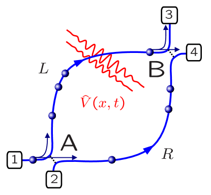
Figure 2: Schematic of the Mach-Zehnder setup, with beam splitters $A,B$, input ports $1,2$, and output ports $3,4$.

Below we will apply our approach to the fermionic Mach-Zehnder interferometer, though the influence of quantum noise on bosonic interferometers (like in LevinsonEMField ) represents another interesting future avenue of research. We note that recently a different kind of quantum Langevin method has been developed for transport through quantum dotsBingDong .

III Application to the Mach-Zehnder interferometer

III.1 Introduction

In contrast to the usual mesoscopic Aharonov-Bohm ring setups, the recently realized Mach-Zehnder interferometer for electronsHeiblumEtAl ; NederHeiblum offers the possibility to study an ideal two-way interference geometry, with chiral single-channel transport and in the absence of backscattering. The loss of visibility with increasing bias voltage or temperature has been observed, and the idea of using shot noise measurements to learn more about potential dephasing/decoherence mechanisms has been introduced. Recent experimental results present a puzzling picture (e.g. oscillations in the visibilityNederHeiblum ), that has not been explained so far. Under the assumption that at least part of the loss in visibility is due to decoherence processes, the observed decrease in visibility with increasing bias voltage is a good indication that Pauli blocking effects are important, as this effect is due to lifting the restrictions of Pauli blocking on the scattering of particles.

On the theoretical side, the loss of interference contrast in the current had been studied for the Mach-Zehnder setupSeelig prior to this experiment. More recently the influence of decoherence on shot noise has been analyzedunserPRL (see levinson for related work in quantum point contact), revealing important differences between phenomenological and microscopic approaches, leading to renewed investigations on the so-called dephasing terminal model DephasingTerminal and calculations of the full counting statistics in the MZ setup FCSMZ . However, all of these works deal with a classical noise field acting on the electrons. Thus, experimentally observed features such as the increase of the dephasing rate with rising bias voltage could not be studied, as this is a true many-body effect (see below).

III.2 The model

We consider a model of spinpolarized fermions, moving chirally and without backscattering through an interferometer at constant speed $v_{F}$ (see Fig. 2). The two beamsplitters $A$ and $B$ connect the fermion fields $\hat{\psi}_{\alpha}$ of the input ($\alpha=1,2$) and output ($\alpha=3,4$) channels to those of the left and right arm ($\alpha=L,R$), which we take to be of equal length $l$:

$$\hat{\psi}_{L}(0,t) = r_{A}\hat{\psi}_{1}(0,t)+t_{A}\hat{\psi}_{2}(0,t)$$ (7)

$$\hat{\psi}_{R}(0,t) = t_{A}\hat{\psi}_{1}(0,t)+r_{A}\hat{\psi}_{2}(0,t)$$ (8)

$$\hat{\psi}_{3}(l,t) = r_{B}e^{i\phi}\hat{\psi}_{L}(l,t)+t_{B}\hat{\psi}_{R}(l,t)$$ (9)

$$\hat{\psi}_{4}(l,t) = t_{B}e^{i\phi}\hat{\psi}_{L}(l,t)+r_{B}\hat{\psi}_{R}(l,t)$$ (10)

The transmission (reflection) amplitudes $t_{A/B}\,(r_{A/B})$ fulfill $t_{j}^{*}r_{j}=-t_{j}r_{j}^{*}$ due to unitarity, and we have included the Aharonov-Bohm phase difference $\phi$. The input fields $\alpha=1,2$ are described by Fermi distributions $f_{1,2}$, where the chemical potential difference defines the transport voltage: $eV=\mu_{1}-\mu_{2}$. We have

$$\left\langle\psi_{\alpha}^{\dagger}(0,0)\psi_{\alpha}(0,t)\right\rangle=\int_{-k_{c}}^{k_{c}}(dk)\,f_{\alpha k}e^{-iv_{F}kt}$$ (11)

(note $\hbar=1$), with a band-cutoff $k_{c}$. Here and in the following, we use the notation $(dk)\equiv dk/(2\pi)$.

The particles are assumed to have no intrinsic interaction, but are subject to an external free bosonic quantum field $\hat{V}$ (linear bath) during their passage through the arms $L,R$: $\hat{H}_{{\rm int}}=\sum_{\lambda=L,R}\int dx\,\hat{V}_{\lambda}(x)\hat{n}_{\lambda}(x)$ with $\hat{n}_{\lambda}(x)=\hat{\psi}_{\lambda}^{\dagger}(x)\hat{\psi}_{\lambda}(x)$.

We focus on the current going into output port $3$, which is related to the density: $\hat{I}(t)=ev_{F}\hat{n}_{3}(t)$ with $\hat{n}_{3}(t)=\hat{\psi}_{3t}^{\dagger}\hat{\psi}_{3t}$, where we take fields $\hat{\psi}_{\alpha t}=\hat{\psi}_{\alpha}(l,t)$ at the position of the final beamsplitter B (except where noted otherwise). In the following we set $e=v_{F}=1$, except where needed for clarity. We thus have

$$\left\langle\hat{I}\right\rangle=R_{B}\left\langle\hat{\psi}_{L}^{\dagger}\hat{\psi}_{L}\right\rangle+T_{B}\left\langle\hat{\psi}_{R}^{\dagger}\hat{\psi}_{R}\right\rangle+e^{i\phi}t_{B}^{*}r_{B}\left\langle\hat{\psi}_{R}^{\dagger}\hat{\psi}_{L}\right\rangle+{\rm c.c.}.$$ (12)

Therefore, the calculation of the average current has been reduced to a calculation of the elements of a density matrix $\left\langle\hat{\psi}_{\lambda^{\prime}}^{\dagger}\hat{\psi}_{\lambda}\right\rangle$ describing the coherence properties of the fermions right at the second beam splitter (after having been subject to the quantum noise field). We have set $T_{B}=|t_{B}|^{2}$ and $R_{B}=1-T_{B}$.

III.3 Influence on the interference contrast

In this section, we will remind the reader of our results for the influence of the quantum bath on the interference term in the current $I(\phi)$. These have already been presented in a brief communicationEPL , but we repeat them here in order to keep the discussion self-contained. They form the basis of the subsequent sections on the current noise.

In order to obtain the interference term in the current, we expand the exponential, Eq. (5), to second order, insert the formal solution, Eq. (6), and perform Wick’s averaging over fermion fields, while implementing a “Golden Rule approximation”, i.e. keeping only terms linear in the time-of-flight $\tau$.

These steps will be explained in more detail below, in Section IV.3, for the case of the current noise, so we do not display them here.

Note that accounting for cross-correlations between the fluctuations in both arms (“vertex-corrections”) is straightforward for a geometry with symmetric coupling to parallel arms at a distance $d$ (assuming $d\ll l$). Then, in the following results (Eqs. (15), (41)-(45), and $\Gamma_{\varphi}$), we have to set $\left\langle\hat{V}\hat{V}\right\rangle=\left\langle\hat{V}_{L}\hat{V}_{L}\right\rangle-\left\langle\hat{V}_{L}\hat{V}_{R}\right\rangle$ and $D^{R}=D_{LL}^{R}-D_{LR}^{R}$. These correlators, of fields being defined on the one-dimensional interferometer arms, actually have to be derived from their threedimensional versions, e.g. $\left\langle\hat{V}_{L}(x,t)\hat{V}_{R}(x^{\prime},t)\right\rangle=\left\langle\hat{V}(x,y+d,z,t)\hat{V}(x^{\prime},y,z,t^{\prime})\right\rangle$ if the arms are parallel to the $x$-axis and separated in the $y$-direction.

Without bath, the interference term is given by

$$\left\langle\hat{\psi}_{R}^{\dagger}\hat{\psi}_{L}\right\rangle_{(0)}=r_{A}t_{A}^{*}\int(dk)\delta f_{k}=r_{A}t_{A}^{*}(eV/2\pi),$$ (13)

where we define $\delta f_{k}\equiv f_{1k}-f_{2k}$ and $\bar{f}_{k}\equiv(f_{1k}+f_{2k})/2$ (for later).

The leading correction to the interference term can be expressed in terms of a phase-shift and a dephasing rate:

$$\delta\left\langle\hat{\psi}_{R}^{\dagger}\hat{\psi}_{L}\right\rangle=r_{A}t_{A}^{*}\int(dk)\delta f_{k}[i\delta\bar{\varphi}(k)-\Gamma_{\varphi}(k)\tau]$$ (14)

Note that the “classical” contributions $\left\langle\hat{\psi}_{\lambda}^{\dagger}\hat{\psi}_{\lambda}\right\rangle$ (with $\lambda=L,R$) are not affected by the noisy environment. Here the effective average phase shift induced by coupling to the bath is energy-dependent, and given by:

$$\delta\bar{\varphi}(k)=\tau(R_{A}-T_{A})\int(dq)({\rm Re}D_{q,q}^{R}-D_{0,0}^{R})\delta f_{k-q}\,.$$ (15)

Essentially, the phase shift is due to the effective coupling between the electrons, mediated by the bath (containing Hartree and Fock contributions). For that reason, it depends on the nonequilibrium Fermi distribution (difference) $\delta f$. The phase shift vanishes for $T_{A}=1/2$, since then there is complete symmetry between both arms.

The suppression of the interference term is quantified by the dephasing rate $\Gamma_{\varphi}(k)$, within the Markoff/Golden Rule approximation adopted here. In the case of classical Gaussian noise, the suppression can be evaluated exactly (“to all orders” in the system-bath interaction). It is equal to $\exp(-\left\langle\varphi^{2}\right\rangle/2)$, where $\varphi$ is the phase difference between the two arms of the interferometer, fluctuating due to the action of the noisy potential. For the case of a single particle coupled to a quantum bath, the same suppression factor would be given in general by the overlap of bath states that have evolved under the influence of the particle traveling along the left or the right armSAI . Up to now, we have not been able to find an equally simple interpretation for the many-particle case.

The total dephasing rate is $\Gamma_{\varphi}(k)=\Gamma_{\varphi}^{L}(k)+\Gamma_{\varphi}^{R}(k)$. For equal coupling to both arms, this can be written as:

$$\Gamma_{\varphi}(\epsilon)=\int_{0}^{\infty}\frac{d\omega}{v_{F}}{\rm DOS}_{q}(\omega)[2n(\omega)+1-(\bar{f}(\epsilon-\omega)-\bar{f}(\epsilon+\omega))]$$ (16)

The rate (at energy $\epsilon=\epsilon(k)=v_{F}(k-k_{F})+\epsilon_{F}$) is an integral over all possible energy transfers $\omega$ from and to the bath (which have been combined, so $\omega>0$ here). They are weighted by the bath spectral “density of states” ${\rm DOS}_{q}(\omega)=-{\rm Im}D_{q}^{R}(\omega)/\pi$, where $q=\omega/v_{F}$ for ballistic motion (in this definition, ${\rm DOS}$ has the dimensions $\omega/q$).

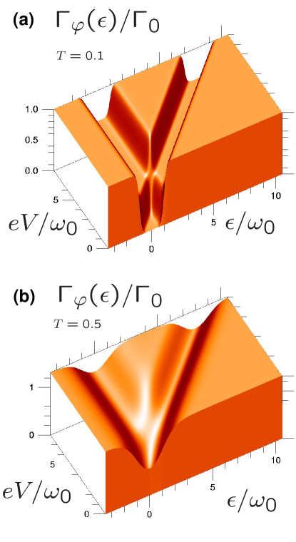
Figure 3: Energy-resolved dephasing rate for an optical phonon mode (at $\omega_{0}$), as a function of transport voltage applied to the Mach-Zehnder, for two different temperatures: (a) $T=0.1\omega_{0}$, (b) $T=0.5\omega_{0}$. Here $\Gamma_{0}=\Gamma_{\varphi}(\epsilon\rightarrow\infty,T=0)$.

The first term in brackets, $2n(\omega)+1$, describes the strength of thermal and quantum fluctuations (with $n(\omega)=(e^{\omega/T}-1)^{-1}$ the Bose-Einstein distribution). It stems from the $\hat{V}_{(0)}$ in the quantum phase. By itself, this would give rise to an energy-independent rate and a visibility independent of bias voltage, in contradiction to experimental results. In fact, such a procedure (dropping the back-action terms) would describe a different physical situation: that of a single particle coupled to a quantum bath (in absence of the Fermi sea).

Thus, the second term is crucially important. The “back-action” $\propto D^{R}\hat{n}$ introduces the nonequilibrium Fermi functions ($f_{L}=R_{A}f_{1}+T_{A}f_{2}$, $f_{R}=T_{A}f_{1}+R_{A}f_{2}$, and their average, $\bar{f}=(f_{L}+f_{R})/2=(f_{1}+f_{2})/2$) which capture the physics of Pauli blocking: Large energy transfers $v_{F}|q|\gg eV,T$ are forbidden for states $k$ within the transport voltage window. This can be seen in Fig. 3, which displays the energy-dependence of the dephasing rate, as a function of voltage and temperature. For the simplest example of an optical phonon mode (where only an energy transfer $\omega_{0}$ is allowed), we find two dips in the dephasing rate at large voltages. These occur around the edges of the non-equilibrium Fermi distribution $\bar{f}$, i.e. at the edges of the voltage window, and their width is $2\omega_{0}$. When the voltage is reduced, these two dips merge and the rate goes down to zero. Thus, when averaging this rate over the voltage window (in which electrons contribute to the current), the average rate becomes zero for $V,T\rightarrow 0$. As a result, the interference contrast (visibility) becomes perfect (see also the energy-averaged dephasing rate depicted in EPL ). In contrast, at higher temperature, two effects increase the dephasing rate: First, thermal smearing of the Fermi distributions reduces the restrictions of Pauli blocking, and second, thermal fluctuations in the bath lead to processes of induced emission and absorption.

Note that the strong energy-dependence of the dephasing rate in the many-fermion case is markedly different from the single-particle situation, and thus the dependence on the bath spectrum is completely different as well. In the single-particle case, it is enough to know the variance $\left\langle\varphi^{2}\right\rangle$ of the fluctuating phase difference, in order to calculate the loss of visibility. In the many-particle case, we have to keep track of the full bath spectrum $\left\langle\hat{V}\hat{V}\right\rangle_{q,\omega}$.

As we have only evaluated the corrections to lowest order, we should be able to make contact to Fermi’s Golden Rule, describing the scattering of electrons inside the interferometer arms, by emission or absorption of phonons (bath quanta). Indeed, it turns out that the dephasing rate is related to Golden Rule scattering rates. However, we emphasize that it is not given solely by the rate for scattering of particles, as one might naively assume. Rather, hole-scattering processes provide an equally important contribution to the dephasing rate, which is thus the sum of particle- and hole-scattering rates. In our case, we find:

$$\Gamma_{\varphi}^{L/R}=(\Gamma_{p}^{L/R}+\Gamma_{h}^{L/R})/2,$$ (17)

with $\Gamma_{p}^{L/R}(k)=\int(dq)\,\left\langle\hat{V}\hat{V}\right\rangle_{q,q}(1-f_{L/R,k-q})$ and $\Gamma_{h}^{L/R}(k)=\int(dq)\,\left\langle\hat{V}\hat{V}\right\rangle_{q,q}f_{L/R,k+q}$. This is because both processes destroy the superposition of many-particle states that is created when a particle passes through the first beam splitter, entering the left or the right arm. A more detailed qualitative discussion may be found in JvDAndMe , for the case of weak localization, and in the next subsection.

For linear transport, i.e. a the limit of infinitesimal bias voltage $V\rightarrow 0$, we have $f_{Lk-q}-f_{Lk+q}\rightarrow-\tanh(\beta(k-q)/2)$ under the integral. Then we recover the result well known in the theory of weak localizationWLdephasingDiags , where ballistic motion in our case ($\omega=v_{F}q$) is replaced by diffusion.

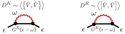
Figure 4: Contributions to the decoherence rate in a Keldysh-diagrammatic treatment. Left: Diagram involving both thermal and quantum fluctuations of the bath, but no Fermi distributions. This diagram is the same in a single-particle situation. Right: Diagram corresponding to the “back-action” term discussed in the equations of motion approach. It involves the fermionic Keldysh Green’s function (that contains the Fermi distribution, $G^{K}(\epsilon-\omega)\propto 1-2f(\epsilon-\omega)$) and the bath’s retarded propagator (describing the response).

Finally, we note that a treatment using Keldysh diagrams would yield (in the absence of vertex corrections) a dephasing rate that is equal to the decay rate of the retarded (or advanced) propagator, and thus given by the sum of the two diagrams shown in Fig. 4. These correspond exactly to the first and the second contribution discussed above. For the average current, the effort involved in both calculations (Keldysh or equations of motion) is still about the same (a few lines). However, for the shot noise corrections discussed below, we found the equations of motion method much more convenient.

III.4 Particle- and hole-scattering contributions to the dephasing rate

In this section, we briefly provide a more qualitative discussion of the fact that hole-scattering processes lead to an equally important contribution to the dephasing rate $\Gamma_{\varphi}=(\Gamma_{p}+\Gamma_{h})/2$. The ratio of $\Gamma_{p}$ and $\Gamma_{h}$ depends on the energy under consideration, with $\Gamma_{p}$ providing the full dephasing rate at high energies, and $\Gamma_{h}$ accounting for $\Gamma_{\varphi}$ at low energies (see EPL ).

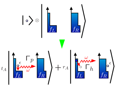
Figure 5: Contribution of particle- and hole-scattering processes to the dephasing rate in a many-fermion interferometer.

This is a generic feature for decoherence of fermionic systems. Even though it is implicit in known diagrammatic resultsWLdephasingDiags , we are not aware of any simple physical discussion (except our own recent treatment JvDAndMe in the case of weak localization). From the perspective of a single particle, the first beam splitter creates a superposition of the form $t_{A}\left|R\right\rangle+r_{A}\left|L\right\rangle$, with the states $R/L$ denoting a wave packet inside the right/left arm. In the presence of a sea of other fermions inside the interferometer arms, we should write instead a superposition of many-body states (see Fig. 5), schematically:

$$t_{A}\left|\ldots,\underline{0},\ldots;\,\ldots,\underline{1},\ldots\right\rangle+r_{A}\left|\ldots,\underline{1},\ldots;\,\ldots,\underline{0},\ldots\right\rangle$$ (18)

We have indicated the occupations $\left|{\rm left};\,{\rm right}\right\rangle$ of single-particle states in both arms, with a bar denoting the energy level $\epsilon$ of interest and the remaining particles (in the nonequilibrium distributions) playing the role of spectators. The interference term $\left\langle\hat{\psi}_{L}^{\dagger}\hat{\psi}_{R}\right\rangle$ is sensitive to the coherent superposition that requires not only the presence of a particle in one arm but also the absence of a particle in the other arm. This is why the many-body superposition can equally be destroyed by particle- and hole-scattering (leading to states with $\left|\ldots,\underline{0},\ldots;\,\ldots,\underline{0},\ldots\right\rangle$ or $\left|\ldots,\underline{1},\ldots;\,\ldots,\underline{1},\ldots\right\rangle$, respectively). We emphasize that the dephasing rate is independent of the amplitudes $t_{A}$ and $r_{A}$ in this superposition. The reason is basically that the dephasing rate describes the decay of the off-diagonal element of the density matrix (in the space of these two states), and that the amplitudes only enter as a constant prefactor in that element. Thus, the dephasing rate is simply given by the sum of particle- and hole-scattering rates, as noted above. The factor $1/2$ arises because we are not asking about the decay of populations (which is described by $\Gamma_{p}$ and $\Gamma_{h}$) but essentially the decay of a wave amplitude. This is the same factor that arises in the relation $T_{2}=2T_{1}$ known for pure dephasing processes in the context of Bloch equations.

IV Current Noise in the Mach-Zehnder setup

IV.1 Introduction

As our method yields directly the modified particle fields, it may be used, in principle, to calculate any higher-order correlator of those fields. Of particular experimental interest is the current noise in the output port of the interferometer. This has been (and is) currently being studied in the Weizmann MZ setupHeiblumEtAl ; NederHeiblum .

IV.2 General properties

The zero-frequency current noise power is defined as

$$S\equiv\int_{-\infty}^{+\infty}dt\,\left\langle\left\langle\hat{I}(t)\hat{I}(0)\right\rangle\right\rangle\,,$$ (19)

where the double bracket denotes the irreducible part: $\left\langle\left\langle\hat{I}(t)\hat{I}(0)\right\rangle\right\rangle=\left\langle\hat{I}(t)\hat{I}(0)\right\rangle-\left\langle\hat{I}\right\rangle^{2}$. For the MZ setup considered here, the current noise only has contributions up to the second harmonic in the external flux:

$$S=S_{0}+S_{1}\cos(\phi-\delta\phi_{1})+S_{2}\cos(2(\phi-\delta\phi_{2})).$$ (20)

The dependence on $\phi$ and $T_{B},R_{B}$ can be made explicit,

$$S=R_{B}T_{B}C_{0}+R_{B}^{2}C_{0R}+T_{B}^{2}C_{0T}+$$ (21)

$$2\textrm{Re}\left[e^{i\phi}(t_{B}^{*}r_{B})(R_{B}C_{1R}+T_{B}C_{1T})-e^{2i\phi}T_{B}R_{B}C_{2}\right]\,.$$

with the coefficients following directly from inserting Eq. (9) into (19), see below. Here $S_{0},S_{1},S_{2},\delta\phi_{1}$ and $\delta\phi_{2}$ can be obtained by comparing Eqs. (21) and (20).

The coefficients $C_{0},C_{0R},\ldots$ are expressed in terms of four-point Green’s functions, similar to the expression for the average current. These, in turn, contain the full dependence on interactions, as well as on voltage, temperature, and $T_{A}$. We list them for reference, setting $L_{t}\equiv\hat{\psi}_{L}(t)$ and $R_{t}\equiv\hat{\psi}_{R}(t)$ for brevity. We will also set $v_{F}\equiv 1$, as before.

$$C_{0R} = \int dt\,\left\langle\left\langle L_{t}^{\dagger}L_{t}L_{0}^{\dagger}L_{0}\right\rangle\right\rangle$$ (22)

$$C_{0T} = \int dt\,\left\langle\left\langle R_{t}^{\dagger}R_{t}R_{0}^{\dagger}R_{0}\right\rangle\right\rangle$$ (23)

$$C_{0} = \int dt\,\left\langle\left\langle L_{t}^{\dagger}L_{t}R_{0}^{\dagger}R_{0}+R_{t}^{\dagger}R_{t}L_{0}^{\dagger}L_{0}\right\rangle\right\rangle+$$ (25)

$$\int dt\,\left\langle\left\langle L_{t}^{\dagger}R_{t}R_{0}^{\dagger}L_{0}\right\rangle\right\rangle+\left\langle\left\langle R_{t}^{\dagger}L_{t}L_{0}^{\dagger}R_{0}\right\rangle\right\rangle$$

$$C_{1R} = \int dt\,\left\langle\left\langle R_{t}^{\dagger}L_{t}L_{0}^{\dagger}L_{0}\right\rangle\right\rangle+\left\langle\left\langle L_{t}^{\dagger}L_{t}R_{0}^{\dagger}L_{0}\right\rangle\right\rangle$$ (26)

$$C_{1T} = \int dt\,\left\langle\left\langle R_{t}^{\dagger}R_{t}R_{0}^{\dagger}L_{0}\right\rangle\right\rangle+\left\langle\left\langle R_{t}^{\dagger}L_{t}R_{0}^{\dagger}R_{0}\right\rangle\right\rangle$$ (27)

$$C_{2} = \int dt\,\left\langle\left\langle R_{t}^{\dagger}L_{t}R_{0}^{\dagger}L_{0}\right\rangle\right\rangle$$ (28)

$C_{0(R/T)}$ are real-valued, the other coefficients may become complex.

In the absence of a quantum bath, these coefficients have the following values:

$$C_{0R/T}^{(0)} = \int(dk)\left[\bar{f}_{k}(1-\bar{f}_{k})-\frac{1}{4}(R_{A}-T_{A})^{2}\delta f_{k}^{2}\right]$$ (29)

$$C_{0}^{(0)} = \int(dk)\left\{f_{Lk}(1-f_{Rk})+f_{Rk}(1-f_{Lk}))\right\}$$ (31)

$$-2R_{A}T_{A}\int(dk)\,\delta f_{k}^{2}$$

$$C_{1R/T}^{(0)} = \pm r_{A}t_{A}^{*}(T_{A}-R_{A})\int(dk)\,\delta f_{k}^{2}\,$$ (32)

$$C_{2}^{(0)} = R_{A}T_{A}\int(dk)\,\delta f_{k}^{2}\,.$$ (33)

Those expressions yield the result given by the well-known scattering theory of shot noise of non-interacting fermions PartitionNoiseOriginal ; BuettikerOriginal ; JongBeenakker ; BlanterBuettiker :

$$S_{(0)}=\int(dk)(f_{2k}+\delta f_{k}\mathcal{T})(1-(f_{2k}+\delta f_{k}\mathcal{T}))\,,$$ (34)

where $\mathcal{T}(\phi)=T_{A}T_{B}+R_{A}R_{B}+2t_{A}^{*}r_{A}t_{B}^{*}r_{B}\cos(\phi)$ is the transmission probability from $1$ to $3$.

For our model, the full shot noise power $S$ may be shown to be invariant under each of the following transformations, if the bath couples equally to both arms of the interferometer: (i) $t_{A}\leftrightarrow r_{A},\,\phi\mapsto-\phi$ (ii) $V\mapsto-V,\,\phi\mapsto-\phi$ (iii) $t_{B}\leftrightarrow r_{B}$. As a consequence, $C_{1T}=-C_{1R}$. Note that the free result (34) is invariant under $\phi\mapsto-\phi$ and $V\mapsto-V$ separately, but these symmetries may be broken by a bath-induced phase-shift, to be discussed below.

IV.3 Evaluation of current noise to leading order in the interaction

In order to evaluate the correlators (22)-(28) to leading order in the interaction, we expand the general solution of the equations of motion for the electron operators. Let $L_{t}^{(0)}$ denote the unperturbed electron field, and $g$ a formal expansion parameter (to be set to $1$ in the end). Then we have, for the electron field at the end of the left arm, just before the final beamsplitter:

$$L_{t} = \left[1-ig\int_{0}^{\tau}dt_{1}\tilde{V}_{L}(t_{1},t)-\right.$$

$$g^{2}\int_{0}^{\tau}dt_{1}\int_{0}^{t_{1}}dt_{2}\,\tilde{V}_{L}(t_{1},t)\tilde{V}_{L}(t_{2},t)-$$

$$ig^{2}\int_{0}^{\tau}dt_{1}\int_{-\infty}^{+\infty}dt_{2}\int_{-\infty}^{+\infty}dx_{2}\,\times$$

$$\left.\tilde{D}_{LL}^{R}(t_{1},t;x_{2},t_{2})\,L_{\tau+t_{2}-x_{2}/v_{F}}^{(0)\dagger}L_{\tau+t_{2}-x_{2}/v_{F}}^{(0)}\right]L_{t}^{(0)}$$

We have expressed the arguments of the potentials $V$ and response kernel $D^{R}$ in terms of the time $t_{1}=0\ldots\tau$ elapsed since entry into the left interferometer arm, with the electron moving from $x=0$ to $x=l=v_{F}\tau$ during the corresponding time-interval $[t-\tau,t]$. We have set

$$\tilde{V}_{L}(t_{1},t) \equiv \hat{V}_{L}(v_{F}t_{1},t-\tau+t_{1})$$ (36)

$$\tilde{D}_{LL}^{R}(t_{1},t;x_{2},t_{2}) \equiv D^{R}(v_{F}t_{1}-x_{2},t-\tau+t_{1}-t_{2})\,,$$ (37)

assuming a stationary environment that is translationally invariant. The expressions for $R_{t}$ are completely analogous. In writing down Eq. (IV.3), we have omitted the cross-term $D_{LR}^{R}$, assuming that the wavelength of relevant fluctuations is considerably shorter than the distance between the arms of the interferometer (such a term can be added easily, see the remark above, in Section III.3). This also implies $\left\langle\hat{V}_{L}\hat{V}_{R}\right\rangle=0$. In terms of the bath spectra, we have (both for $L$ and $R$):

$$\left\langle\tilde{V}_{L}(t^{\prime}_{1},t^{\prime})\tilde{V}_{L}(t_{1},t)\right\rangle=$$

$$\int(dq)\int(d\omega)\,e^{i[(v_{F}q-\omega)(t^{\prime}_{1}-t_{1})-\omega(t^{\prime}-t)]}\left\langle\hat{V}\hat{V}\right\rangle_{q\omega}$$ (38)

$$\tilde{D}_{LL}^{R}(t_{1},t;x_{2},t_{2})=$$

$$\int(dq)\int(d\omega)e^{i[q(v_{F}t_{1}-x_{2})-\omega(t_{1}-t_{2}+t-\tau)]}D_{q\omega}^{R}$$ (39)

We now evaluate the leading order ($g^{2}$) correction to the noise power (21), by inserting the expressions for $L_{t}$ and $R_{t}$ into the coefficients $C_{0},C_{1T},C_{1R},$ and $C_{2}$ (Eqs. (25)-(28)). Bare electron operators are contracted using Wick’s theorem, and the resulting averages can be performed by expressing $L_{t}^{(0)},\,R_{t}^{(0)}$ via $\hat{\psi}_{1,2}$ (Eqs. (7),(8)) and employing Eq. (11). After inserting the Fourier representations $\left\langle\hat{V}\hat{V}\right\rangle_{q\omega}$ and $D_{q\omega}^{R}$, all temporal and spatial integrations have to be carried out. In doing so, we will use a Golden Rule (Markoff) approximation, i.e. we keep only the leading order in $\tau$,

$$\int_{0}^{\tau}dt_{1}\int_{0}^{t_{1}}dt_{2}e^{i\lambda(t_{1}-t_{2})} \approx \tau\frac{i}{\lambda+i0}\,$$ (40)

(and so on), assuming the correlation time of the environment to be much shorter than the time-of-flight $\tau$. Although it is in principle straightforward to go beyond this approximation (evaluating all these integrals exactly), the result gets very unwieldy, and other effects (such as the curvature of the interferometer paths) should be taken into account as well on that refined level of description. Thus, we are neglecting the fact that energy- and momentum-conservation will only be fulfilled up to a Heisenberg uncertainty $\tau^{-1}$ and $l^{-1}$, respectively. Within this approximation, we have been allowed to extend the $x_{2}$-integral in Eq. (IV.3) over all of space, even though the interaction is assumed to be restricted to the interferometer arm (it will be restricted automatically by the short range of $D^{R}$ and the fact that $t_{1}\in[0,\tau]$).

IV.4 Current noise corrections due to the quantum bath

After a straightforward but lengthy calculation, we arrive at the leading-order corrections to the coefficients $C_{0},C_{1R},C_{2}$ in the noise power $S$. Here we list the explicit analytical results for the shot noise correction (cf. Eq. 21), valid for arbitrary bath spectra (note $\delta C_{0R/T}=0$ and $\delta C_{1T}=-\delta C_{1R}$):

$$\frac{\delta C_{0}}{4\tau R_{A}T_{A}}=-\int(dk)(dq)\,{\rm Im}D_{q,q}^{R}\times$$

$$\left[\delta f_{k}\delta f_{k+q}(\bar{f}_{k+q}-\bar{f}_{k})+\right.$$

$$\left.(f_{1k}^{2}+f_{2k}^{2})\bar{f}_{k+q}-(f_{1k+q}^{2}+f_{2k+q}^{2})\bar{f}_{k}\right]+$$

$$\int(dk)(dq)\left\langle\hat{V}\hat{V}\right\rangle_{q,q}\times$$

$$[(f_{1k+q}-f_{1k})(1-f_{1k})+(f_{2k+q}-f_{2k})(1-f_{2k})]$$

$$+(eV/2\pi)^{2}\left\langle\hat{V}\hat{V}\right\rangle_{0,0}\,,$$ (41)

$${\rm Re}\frac{\delta C_{1R}}{\tau r_{A}t_{A}^{*}(R_{A}-T_{A})}=\int(dk)(dq){\rm Im}D_{q,q}^{R}\times$$

$$[\delta f_{k}\delta f_{k+q}(\bar{f}_{k+q}+3\bar{f}_{k}-2)+\delta f_{k+q}^{2}\bar{f}_{k}-\delta f_{k}^{2}\bar{f}_{k+q}]+$$

$$\left[\int(dq)\left\langle\hat{V}\hat{V}\right\rangle_{q,q}\right]\left[\int(dk)\delta f_{k}^{2}\right]\,,$$ (42)

$${\rm Im}\frac{\delta C_{1R}}{\tau r_{A}t_{A}^{*}}=\int(dk)(dq){\rm Re}D_{q,q}^{R}\times$$

$$\left[-\delta f_{k}\delta f_{k+q}(\delta f_{k+q}+2\delta f_{k})(T_{A}-R_{A})^{2}/2+\right.$$

$$2R_{A}T_{A}\delta f_{k}\delta f_{k+q}^{2}+\delta f_{k+q}\bar{f}_{k}(3-2\bar{f}_{k})$$

$$\left.-\delta f_{k}\bar{f}_{k+q}+2\bar{f}_{k}\bar{f}_{k+q}(\delta f_{k}-\delta f_{k+q})\right]$$

$$+D_{0,0}^{R}(eV/2\pi)\int(dk)\times$$

$$\left[\delta f_{k}^{2}(\frac{3}{2}(T_{A}^{2}+R_{A}^{2})-5R_{A}T_{A})-2\bar{f}_{k}(1-\bar{f}_{k})\right]\,,$$ (43)

$$\frac{{\rm Re}\delta C_{2}}{2\tau R_{A}T_{A}}=(eV/2\pi)^{2}\left\langle\hat{V}\hat{V}\right\rangle_{0,0}-$$

$$2\int(dk)(dq)\,{\rm Im}D_{q,q}^{R}\bar{f}_{k}\delta f_{k+q}(\delta f_{k}+\delta f_{k+q})-$$

$$\int(dk)(dq)\left\langle\hat{V}\hat{V}\right\rangle_{q,q}\delta f_{k}(\delta f_{k}+\delta f_{k+q})$$ (44)

$${\rm Im}\delta C_{2}=-4R_{A}T_{A}\int(dk)\delta f_{k}^{2}\delta\bar{\varphi}_{k}\,.$$ (45)

To obtain physical insights, it is best to translate the coefficients that have been obtained above into corrections to the different harmonics $S_{0},S_{1},S_{2}$ of the noise pattern $S(\phi)$ and the phase shifts $\delta\phi_{1}$ and $\delta\phi_{2}$ (compare Eqs. (20) and (21)). Then we find, for the lowest order corrections:

$$\delta S_{0} = R_{B}T_{B}\delta C_{0}$$ (46)

$$\frac{\delta S_{1}}{S_{1}} = \frac{i{\rm Im}\delta C_{1R}}{C_{1R}^{(0)}}$$ (47)

$$\frac{\delta S_{2}}{S_{2}} = \frac{{\rm Re}\delta C_{2}}{C_{2}^{(0)}}$$ (48)

$$\delta\phi_{1} = \frac{i{\rm Re}\delta C_{1R}}{C_{1R}^{(0)}}$$ (49)

$$\delta\phi_{2} = -\frac{{\rm Im}\delta C_{2}}{C_{2}^{(0)}}$$ (50)

(Note, when comparing with Eqs. (42) and (43), that we took into account $r_{A}t_{A}^{*}$, and thus also $C_{1R}^{(0)}$, being purely imaginary)

IV.5 Discussion of current noise in the Mach-Zehnder coupled to a quantum bath

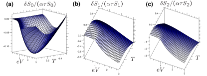
Figure 6: (a) Correction to the flux-averaged current noise power $S_{0}$ for a damped optical phonon mode (strength $\alpha$, time-of-flight $\tau$), normalized with respect to unperturbed value. (b) and (c): The corrections to the first and second harmonics $S_{1}$ and $S_{2}$ are negative, revealing the loss of interference contrast in $S(\phi)$. Energies are plotted in units of the phonon mode ($\omega_{0}=1$), and the MZ setup has been chosen asymmetric ($T_{A}=0.3,T_{B}=0.4$).

The results of evaluating Eqs. (46)-(50) are shown in Figs. (6) and (7) for the illustrative example of a damped optical phonon mode, $D_{q,\omega}^{R}=\alpha[(\omega-\omega_{0}+i\eta)^{-1}-(\omega+\omega_{0}+i\eta)^{-1}]$, with $\eta/\omega_{0}=0.1$.

As expected, the $\phi$-dependence of the shot noise (21) is suppressed, i.e. not only the visibility (interference contrast) of the current pattern $I(\phi)$ but also that of the shot noise pattern $S(\phi)$ is reduced by the bath: see Fig. 6 (b) and (c). We emphasize that this reduction becomes noticeable only once the voltage or the temperature become comparable to the frequency of the phonon mode. Only then the particle can lose its coherence by leaving a trace in the bath (that acts as a kind of “which-way detector”). This is the same behaviour found for the visibility of the current, and it is satisfying that this simple qualitative physical idea also holds for decoherence in shot noise. Note, however, that we have not found a way to express the comparatively complicated formulas for $\delta S_{1}$ and $\delta S_{2}$ in terms of the simple dephasing rate which we derived above, Eq. 16. It is interesting to note that the decrease of the second harmonic $S_{2}$ proceeds faster than that of the first harmonic, $S_{1}$. This is qualitatively consistent with the observations made by Chung et al. for a MZ setup using the phenomenological dephasing terminal modelchung .

There is no Nyquist noise correction, as seen in Fig. 6 (a), at $V=0$. This can be understood easily, since the (unperturbed) Nyquist noise $S_{(0)}(V=0)$ does not depend on $\phi$ and thus should not be sensitive to a noisy environment that changes the phase $\phi$.

The limit of classical noise (treated to all orders in Refs. unserPRL ) is recovered by setting $D^{R}=0$ and using the symmetrized correlator $\left\langle V_{{\rm cl}}V_{{\rm cl}}\right\rangle=\left\langle\left\{\hat{V},\hat{V}\right\}\right\rangle/2$ everywhere in the shot noise correction derived here, with the exception of Eq. (41), which has to be replaced by:

$$\frac{\delta C_{0}^{{\rm cl}}}{\tau}=2\int(dk)(dq)\left\langle V_{{\rm cl}}V_{{\rm cl}}\right\rangle_{q,q}\times$$

$$[(f_{Lk+q}-f_{Lk})(1-f_{Rk})+(f_{Rk+q}-f_{Rk})(1-f_{Lk})]+$$

$$4R_{A}T_{A}\left[\int(dk)\,\delta f_{k}\right]^{2}\left\langle V_{{\rm cl}}V_{{\rm cl}}\right\rangle_{0,0}\,.$$ (51)

This contribution contains a finite $\phi$-independent Nyquist noise correction (cf. unserPRL ), in contrast to our result for the quantum bath. This may be understood as being due to heating of the MZ electrons by a bath which is nominally at infinite temperature (according to the fluctuation-dissipation theorem FDT, applied to the case $D^{R}=0$).

We emphasize that it is impossible to recover the full quantum noise result by inserting some suitably modified classical noise correlator $\left\langle V_{{\rm cl}}V_{{\rm cl}}\right\rangle$. This is in contrast to the dephasing rate, where such a procedure (with $\left\langle V_{{\rm cl}}V_{{\rm cl}}\right\rangle$ containing Fermi functions for Pauli blocking, see Refs. JvDAndMe or alsoCohenImry ) can be made to work. In particular, having only classical noise cannot yield the important phase shift terms. In contrast, the conductance fluctuations are correctly captured even by the classical approach.

At large $V$ (larger than the bath spectrum cutoff), there is a contribution $\propto V^{2}$ in $\delta S_{0}$ and $\delta S_{2}$, due to time-dependent conductance fluctuations ($\delta I\propto\delta G(\phi(t))\cdot V$), corresponding to the leading order of “$S_{{\rm cl}}$” in Refs. unserPRL (see $\left\langle\hat{V}\hat{V}\right\rangle_{0,0}$ terms in Eqs. (41) and (44)).

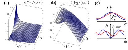
Figure 7: Corrections to the phase shifts $\delta\phi_{1}$ (a) and $\delta\phi_{2}$ (b) of the first and second harmonic in the shot noise pattern $S(\phi)$, in an asymmetric MZ setup (parameters as in Fig. 6). These phase shifts will, in general, be different from the effective phase shift $\delta\bar{\varphi}$ in the current pattern, leading to the situation schematically depicted in (c).

As mentioned in EPL the main surprising feature connected to the shot noise correction is the behaviour of the phase-shifts $\delta\phi_{1,2}$. Naively, one might expect the effective phase shift to be one and the same for all quantities depending on the Aharonov-Bohm phase, whether it be the current $I(\phi)$ or the shot noise $S(\phi)$. However, the phase-shift $\delta\phi_{2}$ in the $e^{2i\phi}$ term is twice as large as expected from the phase-shift in $I(\phi)$ and, moreover, the $e^{i\phi}$ phase-shift $\delta\phi_{1}$ does not vanish even if $T_{A}=1/2$ (but $T_{B}\neq 1/2$). As a consequence, and in contrast to the current $I(\phi)$, even for completely symmetric interferometer arms (same density, same Fermi distributions, same coupling to the bath), there remains a $\phi\leftrightarrow-\phi$-asymmetry in $\delta S$. The explanationEPL rests on the fact that the phase shift is sensitive to the density difference between the arms (as discussed above). As a consequence, density fluctuations in both arms also lead to fluctuations of this phase shift. While the average current only feels the average phase shift $\delta\bar{\varphi}$, the current noise is affected by those fluctuations. The extra terms in $\delta S$, which are responsible for the deviation from the behaviour of the average current, come about because the fluctuations of the phase shift are correlated with the output current, $\left\langle(\delta\hat{\varphi}(t)-\delta\bar{\varphi})(\hat{I}(0)-\bar{I})\right\rangle\neq 0$. This is a straightforward consequence of the fact that the output current $\hat{I}$ itself is correlated with the currents/densities traveling inside the interferometer arms. This also explains the fact that $T_{A}=1/2$ is not enough to obtain a $\phi$-symmetric shot noise (since the correlator $\left\langle\delta\hat{\varphi}\hat{I}\right\rangle$ depends on $T_{B}$ as well).

We emphasize that a fluctuating effective phase shift depending on the density fluctuations inside the arms will quite likely be present in any model of interacting fermions moving inside an interferometer (either with intrinsic interactions, i.e. as a Luttinger liquidLawFeldmanGefen , or with interactions mediated by a bath, like in the present work). Thus, the consequences (different phase shifts in current and current noise, and different phases of the two harmonics in the current noise) will hold more generally than our specific model. It is thus important to carry out experiments that test for those phase shifts in asymmetric interacting interferometers.

IV.6 Conclusions

We have presented an equations of motion (quantum Langevin) approach to ballistic interferometers containing many particles coupled to a quantum bath. It takes into account the simplifications provided by the chiral motion at approximately constant velocity, and is thus more efficient than more general approaches. In particular, it is able to keep, in a straightforward and physically transparent manner, many-body effects, such as Pauli blocking (described as a consequence of the backaction of the bath onto the system) or the influence of hole-scattering processes in the case of fermions. We have applied this method to the fermionic Mach-Zehnder interferometer, presenting full analytical results for the influence of the quantum bath on the current noise. As we have discussed, the main effects are a reduction of the interference contrast in the shot noise pattern $S(\phi)$ and a peculiar behaviour of the effective phase shifts in the two harmonics of $S(\phi)$, for asymmetric setups.

We are anticipating future applications such as the treatment of higher-order effects of the bath or decoherence in bosonic (atom-chip) interferometers.

- (1) A. O. Caldeira and A. J. Leggett, Physica 121A, 587 (1983); Phys. Rev. A 31, 1059 (1985).
- (2) U. Weiss: Quantum Dissipative Systems, World Scientific, Singapore (2000).
- (3) A. H. C. Neto, C. D. Chamon, C. Nayak, Phys. Rev. Lett. 79, 4629 (1997).
- (4) I. L. Aleiner, N. S. Wingreen, and Y. Meir, Phys. Rev. Lett. 79, 3740 (1997).
- (5) F. Marquardt and C. Bruder, Phys. Rev. B 65, 125315 (2002).
- (6) F. Marquardt and C. Bruder, Phys. Rev. B 68, 195305 (2003).
- (7) F. Marquardt and D. S. Golubev, Phys. Rev. Lett. 93, 130404 (2004); Phys. Rev. A 72, 022113 (2005).
- (8) F. Marquardt, Europhys. Lett. 72, 788 (2005).
- (9) Y. Ji, Y. Chung, D. Sprinzak, M. Heiblum, D. Mahalu, and H. Shtrikman, Nature 422, 415 (2003).
- (10) F. Marquardt and C. Bruder, Phys. Rev. Lett. 92, 056805 (2004); Phys. Rev. B 70, 125305 (2004).
- (11) Y. Levinson, J. Phy. A 37, 3003 (2004).
- (12) Bing Dong, Norman J.M. Horing, H.L. Cui, Phys. Rev. B 72, 165326 (2005).
- (13) I. Neder, M. Heiblum, Y. Levinson, D. Mahalu, and V. Umansky, Phys. Rev. Lett. 96, 016804 (2006).
- (14) G. Seelig and M. Büttiker, Phys. Rev. B 64, 245313 (2001).
- (15) Y. Levinson and P. Wölfle, Phys. Rev. Lett. 83, 1399 (1999).
- (16) S. Pilgram, P. Samuelsson, H. Förster, M. Büttiker, cond-mat/0512276.
- (17) H. Förster, S. Pilgram, and M. Büttiker, Phys. Rev. B 72, 075301 (2005).
- (18) A. Stern, Y. Aharonov, and Y. Imry, Phys. Rev. A 41, 3436 (1990).
- (19) F. Marquardt, J. v. Delft, R. Smith, and V. Ambegaokar, cond-mat/0510556.
- (20) H. Fukuyama and E. Abrahams, Phys. Rev. B 27, 5976 (1983); I. Aleiner, B. L. Altshuler, and M. E. Gershenzon, Waves in Random Media 9, 201 (1999) [cond-mat/9808053]
- (21) V. A. Khlus, Zh. Eksp. Teor. Fiz. 93, 2179 (1987); G. B. Lesovik, JETP Lett. 49, 592 (1989)
- (22) M. Büttiker, Phys. Rev. Lett. 65, 2901 (1990); Phys. Rev. B 46, 12485 (1992)
- (23) M. J. M. de Jong and C. W. J. Beenakker, in Mesoscopic Electron Transport, ed. by L. P. Kouwenhoven et al., NATO ASI Series Vol. 345 (Kluwer Academic, Dordrecht, 1997)
- (24) Ya. M. Blanter and M. Büttiker, Phys. Rep. 336, 1 (2000).
- (25) V. S.-W. Chung, P. Samuelsson, and M. Büttiker, Phys. Rev. B 72, 125320 (2005).
- (26) D. Cohen and Y. Imry, Phys. Rev. B 59, 11143 (1999).
- (27) K. T. Law, D. E. Feldman, and Yu. Gefen, cond-mat/0506302.