Distance traveled by random walkers before absorption in a random medium

Abstract

We consider the penetration length $l$ of random walkers diffusing in a medium of perfect or imperfect absorbers of number density $\rho$. We solve this problem on a lattice and in the continuum in all dimensions $D$, by means of a mean-field renormalization group. For a homogeneous system in $D>2$, we find that $l\sim\max\left(\xi,\rho^{-1/2}\right)$, where $\xi$ is the absorber density correlation length. The cases of $D=1$ and $D=2$ are also treated. In the presence of long-range correlations, we estimate the temporal decay of the density of random walkers not yet absorbed. These results are illustrated by exactly solvable toy models, and extensive numerical simulations on directed percolation, where the absorbers are the active sites. Finally, we discuss the implications of our results for diffusion limited aggregation (DLA), and we propose a more effective method to measure $l$ in DLA clusters.

I Introduction

The dynamics of random walkers diffusing in the presence of a finite density of perfect absorbers is a rich problem which has been widely discussed in the physical and mathematical literature donsker . At very large times, the density of surviving walkers does not decay exponentially as a simple mean-field argument would predict, but rather behaves as

$$n(t)\sim\exp\left[-C_{D}\rho^{\frac{2}{D+2}}t^{\frac{D}{D+2}}\right],$$ (1)

where $\rho$ is the absorber density, and $C_{D}$ is a numerical constant. The physical interpretation is that the process is dominated by particles starting in very large absorber-free regions (voids), of linear size $L$. In $D$ dimensions, these regions have a probability of order

$$\exp(-\rho L^{D}),$$ (2)

for small $\rho$. In a void of size $L$, solving the diffusion equation with absorbing conditions on its surface shows that the density typically decays as $\exp(-t/L^{2})$. A saddle-point argument then leads to the result of Eq. (1), with the relevant regions being of typical size $L\sim(t/\rho)^{\frac{1}{D+2}}$, at time $t$.

Another important question is the determination of the penetration or screening length $l$, which measures the average distance between the starting point and the absorption point. In the limit of a small density of uniformly distributed perfect absorbers of radius $a$, and for $D>2$, a classic result muka states that

$$l\sim\frac{a^{1-D}}{\rho}.$$ (3)

However, a simple heuristic argument casts doubts on the validity of Eq. (3). In $D$ dimensions, let us consider a hypercubic box of linear size $L\sim\rho^{-1/D}$, which is the typical distance between absorbers. We place one absorber of radius $a$ in this box, and impose periodic boundary conditions, which is equivalent to copying the box periodically. We now release a random walker at time $t=0$. To estimate the typical time when the walker will hit the absorber, we partition our box in smaller boxes of size $a^{D}$. The random walker will be absorbed with a finite probability once it has visited most of these small cells, including in particular the one containing the absorber. We define $N_{D}(t)$ as the number of different sites visited by a discrete random walker after a time $t$. Hence, a fair estimate of the absorbing time $t_{*}$ is given by

$$N_{D}(t_{*})\sim\left(\frac{L}{a}\right)^{D}\sim(\rho a^{D})^{-1}.$$ (4)

During this time, the random walker has traveled a typical distance $l$ given by

$$l\sim\sqrt{\kappa t_{*}},$$ (5)

where $\kappa$ is the diffusion constant. We can use the classical estimates for $N_{D}(t)$ itzy ; feller , which read

$$N_{1}(t) \sim \frac{\sqrt{\kappa t}}{a},\qquad D=1,$$ (6)

$$N_{2}(t) \sim \frac{\kappa t}{a^{2}\ln(\kappa t\,a^{-2})},\qquad D=2,$$ (7)

$$N_{D}(t) \sim \frac{\kappa t}{a^{2}},\qquad D>2.$$ (8)

Finally, combining Eqs. (4,5,6,7,8), we obtain the qualitative estimates

$$l \sim \rho^{-1},\qquad D=1,$$ (9)

$$l \sim \sqrt{-\frac{\ln(\rho a^{2})}{\rho}},\qquad D=2,$$ (10)

$$l \sim \frac{a^{1-D/2}}{\sqrt{\rho}},\qquad D>2.$$ (11)

In the present work, we will justify on more solid theoretical grounds the results of Eqs. (9,10,11). In section II, we introduce a general formalism in order to compute $l$ and the distribution of distances traveled before absorption. In section III, we define an exact renormalization group for the Green’s function on a lattice. This recursion is solved using a mean-field (or cavity-like) approximation and our result confirms the estimates of Eqs. (9,10,11). In the limit $\rho\to 0$, we also address the effect of imperfect absorbers, which becomes relevant in $D>2$. In section IV, we extend this approach to the continuum. We compute the distribution of the distances of absorption and its first moments. The theory is found to be in excellent agreement with numerical simulations in $D=2$ and $D=3$. In section V, we apply our renormalization approach to the case of a strongly correlated distribution of absorbers, characterized by a power law decay of the absorber density correlation function, $c(r)\sim r^{-\alpha}$, up to the correlation length $\xi$. For $\alpha<2$ and $D>1$ (and for $\alpha<1$, in $D=1$), the penetration length is found to be of the same order as $\xi$, $l\sim\xi$. However, for $\alpha>2$, correlation are weak enough, so that the uncorrelated result of Eqs. (9,10,11) is recovered. This result is illustrated by the exact solution of the problem in $D=1$, and exactly solvable toy models in higher dimensions. In addition, we test our ideas on the strongly correlated distribution of active sites in directed percolation simulations performed at the critical point, in $D=2$ and $D=3$. Random walkers absorbed by the active sites are found to have a screening length $l\sim\xi$, whereas the uncorrelated result is recovered above the critical dimension $D_{c}=4$, when correlations become irrelevant. As a conclusion of this section, we extend the result of Eq. (1) to the case of a strongly correlated density of absorbers. In section VI, we discuss the determination of the screening length $l$ for diffusion limited aggregation (DLA) clusters. We emphasize that the most common method to measure $l$ seems inappropriate and we propose an improved scheme. Finally, we give some heuristic arguments inspired by the results of the previous sections, leading to the estimate $l\sim R$, for DLA clusters of gyration radius $R$.

II General Backward Fokker-Planck Formalism

In a $D$-dimensional space, we consider a Brownian particle with diffusion constant $\kappa$. Let $V({\bf x})$ be a positive killing field such that if the Brownian particle is a the position ${\bf x}$, then in the next time interval $dt$, it is killed with probability $V({\bf x})\,dt$. If the particle is not killed, it just keeps on diffusing. We define $P({\bf x},{\bf y})$ as the probability density that, starting from ${\bf x}$, that the particle’s last resting place, i.e. where it is killed or absorbed, is at ${\bf y}$. The quantity $P({\bf x},{\bf y})$ can be calculated by standard backward Fokker-Planck techniques. We consider what happens in the first time step $dt$. One possibility, occurring with probability $V({\bf x})\,dt$, is that the particle is killed where it starts. The other possibility is that it is not killed, this with probability $1-V({\bf x})\,dt$, and so can then make a Brownian jump $d{\bf B}$ having a component in the spatial direction $\mu$, $dB_{\mu}$, obeying $\langle dB_{\mu}dB_{\mu^{\prime}}\rangle=2\kappa\delta_{\mu\mu^{\prime}}dt$. Putting this together gives

$$P({\bf x},{\bf y})=\delta({\bf x}-{\bf y})V({\bf x})dt+\left(1-V({\bf x})dt\right)\langle P({\bf x}+d{\bf B},{\bf y})\rangle.$$ (12)

Expanding to order $dt$, and taking the expectation value over $d{\bf B}$, we obtain

$$-\kappa\nabla_{\bf x}^{2}P({\bf x},{\bf y})+V({\bf x})P({\bf x},{\bf y})=\delta({\bf x}-{\bf y})V({\bf y}).$$ (13)

The solution to Eq. (13) is given by

$$P({\bf x},{\bf y})=G({\bf x},{\bf y})V({\bf y}),$$ (14)

where $G$ is the Green’s function obeying

$$-\kappa\nabla_{\bf x}^{2}G({\bf x},{\bf y})+V({\bf x})G({\bf x},{\bf y})=\delta({\bf x}-{\bf y}).$$ (15)

Note that the derivation of a probability density rather than a probability always requires a bit of care and our above derivation can be made more rigorous by defining an interval $A$ around the point ${\bf y}$ then computing the probability that the particle is killed in $A$ then taking the limit $A\to 0$. One can check that $P$ is normalized as follows. Clearly the operator acting on $G$ in its defining equation Eq. (15) is self-adjoint, which means that $G({\bf x},{\bf y})=G({\bf y},{\bf x})$. Integrating Eq. (15) over all ${\bf x}$, and if the potential $V$ is sufficiently strong, the first term of Eq. (15) will give an irrelevant surface term. We thus obtain

$$\int d{\bf x}\,V({\bf x})G({\bf x},{\bf y})=1.$$ (16)

However $G$ is symmetric which ensures that

$$\int d{\bf y}\,V({\bf y})G({\bf x},{\bf y})=\int d{\bf y}\,P({\bf x},{\bf y})=1,$$ (17)

and which demonstrates the correct normalization of $P$. To further simplify this problem and reduce everything to the study of the Green’s function, we write $H({\bf x},{\bf y})=-\kappa\nabla_{\bf x}^{2}\delta({\bf x}-{\bf y})$ and consider $V$ as an operator, $V({\bf x},{\bf y})=\delta({\bf x}-{\bf y})V({\bf y})$. Using operator notation, $P$ is given by

$$P=[H+V]^{-1}V=[H+V]^{-1}[H+V-H]=I-[H+V]^{-1}H,$$ (18)

which reads, in coordinate notation,

$$P({\bf x},{\bf y})=\delta({\bf x}-{\bf y})+\kappa\nabla^{2}_{\bf y}G({\bf x},{\bf y}).$$ (19)

Now defining the disorder-averaged values of $P$ and $G$ by $p$ and $g$ respectively, we can write the averaged form of the above equation for a translational invariant distribution of absorbers

$$p({\bf y})=\delta({\bf y})+\kappa\nabla^{2}_{\bf y}g({\bf y}).$$ (20)

If the disorder is isotropic, we will have $p({\bf y})=p(y)$, where $y=|{\bf y}|$, and likewise for $g$. The disordered averaged moments of the distance traveled before the particle is killed are more suitably obtained from $\tilde{p}$, the Fourier transform of $p$ defined as

$${\tilde{p}}({\bf k})=\int d{\bf x}\exp(-i{\bf k}\cdot{\bf x})p({\bf x}).$$ (21)

If we write the Fourier transform of $g$, $\tilde{g}$ as

$${\tilde{g}}(k)={1\over\kappa k^{2}+\kappa\Sigma(k)},$$ (22)

where $\kappa\Sigma(k)$ is given by the one particle irreducible diagrams, we then obtain

$${\tilde{p}}(k)={\Sigma(k)\over k^{2}+\Sigma(k)}.$$ (23)

Now, for small $k$ and to leading order, we expect that

$$\Sigma(k)\approx m^{2}+{\delta\kappa\over\kappa}k^{2}+O(k^{4}),$$ (24)

where $m$ is the inverse effective screening length of the averaged Green’s function and $\delta\kappa$ is the renormalization of the diffusion constant. The resulting small $k$ expansion for $\tilde{p}$ is

$${\tilde{p}}(k)\approx 1-{k^{2}\over m^{2}}+O(k^{4}),$$ (25)

so if ${\bf Y}$ is the position where a particle released at the origin is observed, then the disorder averaged second moment of ${\bf Y}$ is simply given by

$$\overline{\langle{\bf Y}^{2}\rangle}={2D\over m^{2}}.$$ (26)

The characteristic distance from the starting position, $l$, at which the particle gets absorbed is therefore the same as the screening length for the Green’s function. We thus define

$$l=\sqrt{\overline{\langle{\bf Y}^{2}\rangle}}={\sqrt{2D}\over m}\sim m^{-1}.$$ (27)

On a discrete lattice, the same arguments apply and we find that

$$p({\bf y})=\delta_{{\bf y},{\bf 0}}+\nabla^{2}g({\bf y}),$$ (28)

where $\nabla^{2}$ denotes the lattice Laplacian. The discrete Fourier transform of $p$ is defined as

$${\tilde{p}}({\bf k})=\sum_{\bf x}\exp(-i{\bf k}\cdot{\bf x})p({\bf x}),$$ (29)

and is given by

$${\tilde{p}}({\bf k})=1+\left[2\sum_{\mu}\cos(k_{\mu})-2D\right]{\tilde{g}}({\bf k}),$$ (30)

on a $D$-dimensional cubic lattice of lattice spacing $a=1$. Now, if we write

$${\tilde{g}}({\bf k})={1\over 2D-2\sum_{\mu}\cos(k_{\mu})+\Sigma({\bf k})},$$ (31)

we find the lattice result, analogous to Eq. (23)

$${\tilde{p}}({\bf k})={\Sigma({\bf k})\over 2D-{2}\sum_{\mu}\cos(k_{\mu})+\Sigma({\bf k})}.$$ (32)

The leading order behavior of $\Sigma$ must be of the form

$$\Sigma({\bf k})\approx m^{2}+\delta\kappa\,k^{2}+O(k^{4}),$$ (33)

thus yielding the lattice result

$$l=\sqrt{\overline{\langle{\bf Y}^{2}\rangle}}={\sqrt{2D}\over m},$$ (34)

which takes the same form as in the continuum. Interestingly, we find that $l$ is not affected explicitly by the renormalization of the diffusion constant $\delta\kappa$.

III Mean-field renormalization group calculation on a lattice

In this section, we will consider a model on the lattice $Z^{D}$ (hence the lattice constant is $a=1$) with a potential $V_{N}({\bf x})$ given by

$$V_{N}({\bf x})=\lambda\sum_{i=1}^{N}\delta_{{\bf x},{\bf a}_{i}}=\sum_{i=1}^{N}U_{i}({\bf x}).$$ (35)

where the ${\bf a}_{i}$’s are absorbing sites, with strength $\lambda$, which are uniformly and independently (in this first instance) distributed among all lattice sites. We denote by ${\cal V}$ the total number of lattice sites.

We now estimate the renormalization of the Green’s function $G_{N}$ for a system with $N$ absorbing sites by the addition of an $N+1$-th absorbing site. A similar method has been introduced in dean to calculate the effective diffusion constant of a tracer particle in a medium composed of randomly placed scatterers. We denote by ${\bf a}_{N+1}$ the position of the newly added absorber. In operator notation, and introducing the discrete Laplacian $H=-\kappa\nabla^{2}$, the discrete version of Eq. (15) for $G_{N}$ and $G_{N+1}$ leads to,

$$(H+V_{N})G_{N} = I,$$ (36)

$$(H+V_{N}+U_{N+1})G_{N+1} = I.$$ (37)

Eliminating $H+V_{N}=G_{N}^{-1}$, we find

$$G_{N}^{-1}G_{N+1}+U_{N+1}G_{N+1}=I.$$ (38)

After multiplying by $G_{N}$ and using the explicit form of $U_{N+1}$, we obtain in coordinates notation,

$$G_{N+1}({\bf x},{\bf y})=G_{N}({\bf x},{\bf y})-\lambda G_{N}({\bf x},{\bf a}_{N+1})G_{N+1}({\bf a}_{N+1},{\bf y}).$$ (39)

If we set ${\bf x}={\bf a}_{N+1}$, we obtain a closed form expression for $G_{N+1}({\bf a}_{N+1},{\bf y})$, which can be substituted into Eq. (39). This leads to the following exact recurrence:

$$G_{N+1}({\bf x},{\bf y})=G_{N}({\bf x},{\bf y})-{\lambda G_{N}({\bf x},{\bf a}_{N+1})G_{N}({\bf a}_{N+1},{\bf y})\over 1+\lambda G_{N}({\bf a}_{N+1},{\bf a}_{N+1})}.$$ (40)

Let us first consider the limit where the absorbing sites kill the particle on contact with probability $1$. This is achieved by taking the limit $\lambda\to+\infty$ and yields

$$G_{N+1}({\bf x},{\bf y})=G_{N}({\bf x},{\bf y})-{G_{N}({\bf x},{\bf a}_{N+1})G_{N}({\bf a}_{N+1},{\bf y})\over G_{N}({\bf a}_{N+1},{\bf a}_{N+1})},$$ (41)

which describes the exact renormalization of the Green’s function due to the addition of a perfect absorber.

If the perfect absorbers are independently distributed, the position ${\bf a}_{N+1}$ is completely uncorrelated with the ${\bf a}_{i}$’s, for $i=1,\cdots,N$. Averaging Eq. (41) over the position ${\bf a}_{N+1}$, but ignoring the correlation between the numerator and the denominator in the second term (a mean-field-like approximation), we obtain

$$G_{N+1}({\bf x},{\bf y})=G_{N}({\bf x},{\bf y})-{\sum_{\bf a}G_{N}({\bf x},{\bf a})G_{N}({\bf a},{\bf y})\over\sum_{\bf a}G_{N}({\bf a},{\bf a})}.$$ (42)

We now perform the average over the remaining particle positions. Using the statistical translational invariance of the system, we find

$$g_{N+1}({\bf y})=g_{N}({\bf y})-{1\over{\cal V}}{\sum_{\bf x}g_{N}({\bf x})g_{N}({\bf y}-{\bf x})\over g_{N}({\bf 0})}.$$ (43)

Taking the Fourier transform of this equation yields

$${\tilde{g}}_{N+1}({\bf k})=\tilde{g}_{N}({\bf k})-{1\over{\cal V}}{\tilde{g}^{2}_{N}({\bf k})\over g_{N}({\bf 0})}.$$ (44)

Defining the density $\rho=N/{\cal V}$, we obtain a differential equation for the evolution of ${\tilde{g}}(\rho,{\bf k})$ in this approximation

$${\partial{\tilde{g}}\over\partial\rho}(\rho,{\bf k})=-{\tilde{g}^{2}(\rho,{\bf k})\over g(\rho,{\bf 0})},$$ (45)

where $g(\rho,{\bf 0})$ is self-consistently given by

$$g(\rho,{\bf 0})=\int_{-\pi}^{\pi}{d{\bf k}\over(2\pi)^{D}}{\tilde{g}}(\rho,{\bf k}).$$ (46)

The solution to Eq. (45,46) with the correct boundary conditions is

$$\tilde{g}(\rho,{\bf k})={\kappa^{-1}\over 2D-2\sum_{\mu}\cos(k_{\mu})+s(\rho)},$$ (47)

where $s(\rho)$ obeys

$${ds\over d\rho}=\left[\int_{-\pi}^{\pi}{d{\bf k}\over(2\pi)^{D}}{1\over 2D-2\sum_{\mu}\cos(k_{\mu})+s(\rho)}\right]^{-1}.$$ (48)

As expected, the defining equation for $s(\rho)$ does not depend on $\kappa$ for perfect absorbers.

Now using the fact that $s(0)=0$, we can integrate Eq. (48) to obtain

$$\int_{-\pi}^{\pi}{d{\bf k}\over(2\pi)^{D}}\ln\left(1+{s(\rho)\over 2D-2\sum_{\mu}\cos(k_{\mu})}\right)=\rho.$$ (49)

For small $s$, we can use standard results for the integral in Eq. (48) itzy . The results depend on the dimensionality and the lattice structure.

• $D=1$: Substituting in the small $s$ behavior of the integral in Eq. (48) itzy , we find

  $${ds\over d\rho}\approx 2\sqrt{s}.$$ (50)

  For small $\rho$, integrating this gives,

  $$s=m^{2}={\rho^{2}},$$ (51)

  which then leads to

  $$l=\frac{\sqrt{2}}{m}=\frac{\sqrt{2}}{\rho}.$$ (52)

  This is clearly the correct scaling in $\rho$, which will be recovered when solving exactly the one dimensional case (see section IV.1). Formally, the result $l\sim\rho^{-1/D}$ holds for any dimension $1\leq D<2$. The physical interpretation is clear: the screening length is simply proportional to the mean distance between absorbers, a result which will only remain true in the absence of strong correlation between them.

• $D=2$: Here we find itzy

  $${ds\over d\rho}\approx-{4\pi\over\ln(s)},$$ (53)

  and integrating this for small $\rho$, we obtain

  $$s=m^{2}\approx-{4\pi\rho\over\ln(\rho)}.$$ (54)

  Hence, the screening length is

  $$l=\frac{2}{m}=\sqrt{-\frac{\ln(\rho)}{\pi\rho}}.$$ (55)

• $D>2$: Here, the leading order is analytic in $\rho$ itzy , and we find

  $${ds\over d\rho}\approx{1\over g(0,{\bf 0})},$$ (56)

  giving

  $$l=\frac{\sqrt{2D}}{m}=\sqrt{\frac{2Dg(0,{\bf 0})}{\rho}}.$$ (57)

  The term $g(0,{\bf 0})$ depends explicitly on the dimension and the lattice structure. For example, for the three dimensional cubic lattice, one has $g(0,{\bf 0})\approx 0.25...$ itzy .

Note that we expect these results to be strongly modified if the absorbers positions are spatially correlated, a problem which will be addressed in section V.

Let us comment on the disagreement between the present results and the one of Ref. muka , presented in Eq. (3). In muka , the author first treats the effect of a single absorber on the free Green’s function. He then assumes that the total correction to $\Sigma({\bf k})$ is simply proportional to the number of absorbers. This statement is in fact incorrect, as absorbers far away from the introduced random walker should have a negligible contribution. Indeed, the walker should be absorbed well before being able to visit the regions where they stand. This is actually the effect of screening, that our renormalization approach effectively captures. In addition, Eq. (18) in Ref. muka , which leads to the final result of Eq. (3), does not make any sense in the small $\rho$ limit, and it seems that the opposite non physical limit was in fact taken.

Finally, we can extend our formalism to the case of imperfect absorbers, corresponding to a finite value of $\lambda$. The penetration length $l$ is now expected to depend explicitly on the diffusion constant $\kappa$. Using Eq. (40), we find that the Green’s function still takes the form of Eq. (47), but with $s(\rho)$ now satisfying

$${ds\over d\rho}=\left[\delta+\int_{-\pi}^{\pi}{d{\bf k}\over(2\pi)^{D}}{1\over 2D-2\sum_{\mu}\cos(k_{\mu})+s(\rho)}\right]^{-1},$$ (58)

with

$$\delta=\frac{\kappa}{\lambda}>0.$$ (59)

In one and two dimensions a random walk is recurrent and visits any position a large number of times. If the density of absorbers is small enough, a particle will visit the first absorber encountered a large number of times before making an excursion sufficiently far away from this first absorber and visiting a region occupied by a different absorber. This means that most particles are absorbed by the first absorber encountered and thus the effect of a finite $\lambda$ should become irrelevant in $D\leq 2$, when $\rho\to 0$.

In $D=1$, we find the explicit result

$$\sqrt{s}+\delta s=\rho,$$ (60)

which leads to

$$l=\frac{2\sqrt{2}\delta}{\sqrt{1+4\delta\rho}-1}.$$ (61)

Hence, for $\rho\ll\delta^{-1}$, we recover the result of Eq. (52).

In $D=2$, Eq. (58) leads to

$$s\left[\delta-{\ln(s)\over 4\pi}\right]=\rho,$$ (62)

or

$$l=\sqrt{-\frac{\ln(\rho)}{\pi\rho}+\frac{4\delta}{\rho}}.$$ (63)

For $\rho\ll\exp(-4\pi\delta)$, we recover the result of Eq. (55).

Finally for $D>2$, considering imperfect absorbers deeply affects the result of Eq. (57). Indeed, we obtain

$$l=\sqrt{\frac{2D(g(0,{\bf 0})+\delta)}{\rho}}.$$ (64)

Note that in all dimensions, we find that the penetration length is an increasing function of $\delta=\frac{\kappa}{\lambda}$, as physically expected.

IV The screening length in the continuum

IV.1 Delta function absorbers in one dimension

We consider a system where the particle performs continuous Brownian motion in one dimension. It makes perfect sense to take an absorbing potential of the form

$$V(x)=\lambda\sum_{i=1}^{N}\delta(x-a_{i}),$$ (65)

corresponding to point-like absorbers. Here, we consider the case where the random walker is absorbed with probability one at each absorbing site, that is to say the limit $\lambda\to+\infty$. Without loss of generality, we set $\kappa=1$, since the final expression of $l$ for perfect absorbers cannot depend on the value of $\kappa$, whatever the spatial dimension. As in the previous section, we apply the cavity approach to calculate the renormalization of the Green’s function by the addition of an extra absorber at $a_{N+1}$. We apply again the method of section III, which leads to the recurrence equation

$${d{\tilde{g}}\over d\rho}=-{{\tilde{g}}^{2}(\rho,k)\over g(\rho,0)},$$ (66)

where the continuous Fourier transform of $g$ is defined as

$$g(\rho,x)={1\over 2\pi}\int_{-\infty}^{\infty}dk\,\exp(ikx){\tilde{g}}(\rho,k).$$ (67)

The solution of Eq. (66) is given by

$${\tilde{g}}={1\over k^{2}+s(\rho)},$$ (68)

where $s$ satisfies

$${ds\over d\rho}=2\sqrt{s},$$ (69)

which leads to $s=m^{2}=\rho^{2}$. Hence, we recover the lattice result

$$l=\frac{\sqrt{2}}{m}=\frac{\sqrt{2}}{\rho}.$$ (70)

We also obtain the explicit form

$${\tilde{p}}(k)={\rho^{2}\over k^{2}+\rho^{2}},$$ (71)

which gives the distribution of $Y$, the displacement from the starting position to the point of absorption, to be

$$p(y)={\rho\over 2}\exp(-\rho|y|).$$ (72)

In fact, in this one dimensional case, the distribution of $Y$ can be computed exactly. A random walker starting from $x=0$, we denote by $b$ the closest absorbing site to the right and by $-a$ the closest absorbing site to the left. Standard results on Brownian motion feller tell us that the probability of hitting $b$ before $-a$ is

$$p_{b}={a\over a+b}.$$ (73)

This means that the probability density function for $Y$ before averaging over the disorder is simply

$$P(y)={a\over a+b}\delta(y-b)+{b\over a+b}\delta(y+a).$$ (74)

The disordered averaged density $p(y)$ is now given by

$$p(y)=\langle P(y)\rangle_{a,b}\,,$$ (75)

where the angled brackets denote the average over the absorber positions $a$ and $b$. If the absorbers are placed as a Poisson point process with rate $\rho$, then the probability density function of $a$ and $b$ is Poissonian

$$w(x)=\rho\exp(-\rho x).$$ (76)

This yields

$$p(y)=\rho\exp(-\rho|y|)\int_{0}^{\infty}dx\,{x\exp(-x)\over x+\rho|y|}=\rho\int_{\rho|y|}^{\infty}dx\left(1-{\rho|y|\over x}\right)\exp(-x),$$ (77)

showing that in this case the relevant length scale in indeed $l\sim\rho^{-1}$. However, we note that the probability density function given by the mean-field renormalization method is not exact in one dimension.

A generalization of this one dimensional model can be constructed as follows. We take the distribution of lengths $L$ between the absorbers to be given by $q(L)$. The average interval length is simply related to the density by

$$\rho^{-1}=\langle L\rangle=\int_{0}^{\infty}dL\,Lq(L).$$ (78)

The probability that the particle starts within an interval of length $L$ has the probability distribution function

$$Q(L)={L\over\langle L\rangle}q(L).$$ (79)

Given that one is in this interval, the position within it is uniformly distributed. This means that we can write $b=L(1-U)$ and $a=LU$, where $U$ is uniformly distributed over $[0,1]$. We thus have

$$P(y)=U\delta(y-L(1-U))+(1-U)\delta(y+LU).$$ (80)

Now performing the disorder average and using the symmetry of the problem, we find

$$p(y) = \int_{0}^{1}du\int_{0}^{\infty}dL\,uQ(L)\,\delta(|y|-(1-u)L),$$ (81)

$$= \int_{0}^{1}du\ {u\over 1-u}Q\left({|y|\over 1-u}\right).$$

Using the explicit form for $Q$ in Eq. (79), we obtain

$$p(y)={\int_{|y|}^{\infty}dx\,\left(1-{|y|\over x}\right)q(x)\over\int_{0}^{\infty}dx\ xq(x)}.$$ (82)

As a check, we set $q(x)=\rho\exp(-\rho x)$ and recover the result Eq. (77), obtained for the memoryless distribution of Poissonian absorbers.

The above method of calculation also allows for a straightforward computation of the moments of $|Y|$ which can be conveniently expressed in terms of the moments of the distribution $q(L)$. We find

$$\langle|Y|^{n}\rangle={2\over(n+1)(n+2)}{\langle L^{n+1}\rangle\over\langle L\rangle}.$$ (83)

In particular, we have

$$l^{2}=\langle|Y|^{2}\rangle=\frac{1}{6}{\langle L^{3}\rangle\over\langle L\rangle},$$ (84)

which gives

$$l=\rho^{-1}=\langle L\rangle,$$ (85)

for uniformly distributed absorbers associated to a Poissonian distribution of intervals.

IV.2 Absorbing spheres in $D\geq 2$

In this section, we compute the behavior of the distance traveled before absorption in two dimensions and above. In this case, we take the absorbers to be spheres of radius $a$. As before, we restrict ourselves to the limit where the density of absorbers $\rho=N/{\cal V}$ is small. As in the case of the lattice system, we denote by $G_{N}$ the Green’s function in the presence of $N$ absorbers and by $G_{N+1}$ the Green’s function obtained when an extra absorber is placed at the point ${\bf a}_{N+1}$ which is uniformly distributed in the volume ${\cal V}$, independently of the other absorbers. We denote by $U_{N+1}({\bf x})$ the potential due to the $N+1$-th absorber which takes the form

$$U_{N+1}({\bf x})=\lambda\,\delta(a-|{\bf x}-\bf{a}_{N+1}|),$$ (86)

where $\lambda$ has the same dimension as $\kappa$ divided by a distance. $U_{N+1}$ is absorbing with strength $\lambda$ on the surface of the sphere of radius $a$ centered at the point ${\bf a}_{N+1}$. In the limit $\lambda\to+\infty$, the absorber is a perfect absorber. Combining Eq. (15) written for $G_{N}$ and $G_{N+1}$, we can find the equation for $G_{N+1}$ in operator notation as

$$G_{N}^{-1}G_{N+1}+U_{N+1}G_{N+1}=I,$$ (87)

which can be rewritten as

$$G_{N+1}({\bf x},{\bf y})=G_{N}({\bf x},{\bf y})-\int d{\bf z}\,G_{N}({\bf x},{\bf z})U_{N+1}({\bf z})G_{N+1}({\bf z},{\bf y}).$$ (88)

The corresponding equation on the lattice was easy to solve as the potential was given by a delta function. However, here we must resort to a further approximation: we assume that we can set $G_{N}({\bf x},{\bf z})\approx G_{N}({\bf x},{\bf a}_{N+1})$ and $G_{N}({\bf z},{\bf y})\approx G_{N}({\bf a}_{N+1},{\bf y})$ in the above integral over the surface of a sphere centered at ${\bf a}_{N+1}$. We obtain

$$G_{N+1}({\bf x},{\bf y})=G_{N}({\bf x},{\bf y})-{\lambda\sigma(D)a^{D-1}G_{N}({\bf x},{\bf a}_{N+1})G_{N}({\bf a}_{N+1},{\bf y})\over 1+\int d{\bf z}\,U_{N+1}({\bf z})G_{N}({\bf z},{\bf a}_{N+1})},$$ (89)

where $\sigma(D)$ is the area of a sphere of unit radius in $D$ dimensions. We cannot make the same approximation for the integral in the denominator as the resulting term would be proportional to $G_{N}({\bf a}_{N+1},{\bf a}_{N+1})$ which is finite on a lattice, but diverges in the continuous case for $D\geq 2$. The finite radius of the absorbing spheres regularizes the result. Now, in the limit of large $\lambda$, we obtain the expression for the renormalization group flow

$$G_{N+1}({\bf x},{\bf y})=G_{N}({\bf x},{\bf y})-{\sigma(D)a^{D-1}G_{N}({\bf x},{\bf a}_{N+1})G_{N}({\bf a}_{N+1},{\bf y})\over\int d{\bf z}\,I({\bf z},{\bf a}_{N+1})G_{N}({\bf z},{\bf a}_{N+1})},$$ (90)

where

$$I({\bf x},{\bf a}_{N+1})=\delta(a-|{\bf x}-\bf{a}_{N+1}|).$$ (91)

Following the same line of arguments as in the lattice case, we find that the disorder averaged Green’s function obeys

$${d{\tilde{g}}\over d\rho}=-{{\tilde{g}}^{2}(\rho,k)\over g(a)},$$ (92)

where we have used the spherical symmetry of the disorder averaged Green’s function. For $\kappa=1$, the solution to this equation is

$${\tilde{g}}={1\over k^{2}+s},$$ (93)

where $s$ obeys

$${d{s}\over d\rho}={1\over g(a)},$$ (94)

and where $g(a)$ has to be computed self-consistently.

• $D=2$: In two dimensions, we have

  $$g(r)={1\over 2\pi}K_{0}(\sqrt{s}r),$$ (95)

  where $K_{0}(x)$ is the Bessel function of the second kind of order 0 abrom . We thus have

  $${d{s}\over d\rho}={2\pi\over K_{0}(\sqrt{s}a)}.$$ (96)

  Assuming that $s$ is sufficiently small, i.e. for sufficiently small $\rho$, we can use the small argument asymptotic form of $K_{0}$ abrom , $K_{0}(u)\sim-\ln(u)$, to obtain

  $${d{s}\over d\rho}={4\pi\over-\ln(sa^{2})},$$ (97)

  where a cut-off of order $a^{2}$ naturally arises. This equation can be integrated up to the leading order, yielding

  $$m^{2}=s\approx-{4\pi\rho\over\ln(\rho a^{2})}.$$ (98)

  We thus find the same functional form as in the lattice case. After some algebra, we find the following results for the lowest order moments:

  $$\langle|{\bf Y}|\rangle={1\over 4}\sqrt{-\pi{\ln(\rho a^{2})\over\rho}},$$ (99)

  and

  $$l=\sqrt{\langle{\bf Y}^{2}\rangle}=\sqrt{-{\ln(\rho a^{2})\over\pi\rho}}.$$ (100)

  The above calculation actually gives the full distribution for ${\bf Y}$. If $r=|{\bf Y}|$, then the probability density function for $R$ is given by

  $$p(r)=m^{2}rK_{0}(mr),$$ (101)

  where $m$ is given by Eq. (98). In the case of imperfect absorbers (finite $\lambda$), the present results are not affected provided that $\rho$ is small enough ($-\delta/\ln(\rho)\ll 1$).

  In Fig. 1, we plot the two first moments of ${\bf Y}$, as found from numerical simulations. We find a perfect agreement with Eqs. (99,100), indicating that the theoretically predicted constant prefactors of the $\rho$ dependence are in fact probably exact in the small density limit. Numerically, in order to access to the low density regime, we use the following algorithm which has been introduced in the context of DLA meakin . Before performing the next move of our Brownian walker, we look for the nearest absorber (by inspection of a grid keeping track of the coarse-grained absorber density), say found at the distance $d$. We then deposit the random walker anywhere on the circle of radius $d-a$ centered at its current position. Indeed, the first position where the walker would cross the perimeter is uniformly distributed on the circle. The random walker is absorbed when the new distance to its nearest absorber is $d\leq a(1+\varepsilon)$, where $\varepsilon$ is small enough (typically, we took $\varepsilon\leq 10^{-3}$, and $a=1$). Note that if we were to actually simulate the random walker trajectory before it reaches the perimeter, the program would take a running time larger by a factor $d^{2}/dt$, where $dt$ is the time increment. When accessing to density of order $\rho\sim 10^{-6}$, and using a time step of order $dt\sim 10^{-3}$, this factor is of order $10^{9}$, which gives an idea of the huge gain achieved by using this algorithm. All the simulations performed in this paper use variants of this algorithm.

  

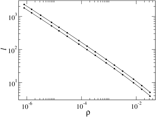
  Figure 1: Plot of $\langle|{\bf Y}|\rangle$ (bottom full circles) and $l=\sqrt{\langle{\bf Y}^{2}\rangle}$ (top full circles) obtained from numerical simulations in $D=2$. Each point is obtained from the average over at least $10^{6}$ random walker trajectories, and we used several samples totalizing at least $10^{6}$ uniformly distributed absorbers. Error bars are much smaller than the size of the circles. We compare these data to the functional forms of Eqs. (99,100) (full lines), with the cut-off $a^{2}$ being the sole fitting parameter. For spheres of radius $a=1$, we find that both curves are well fitted with an effective value of $a^{2}\approx 2.2$.

• $D=3$: In this case, we find

  $$g(r)={1\over 4\pi r}\exp(-\sqrt{s}r).$$ (102)

  For small $s$, Eq. (94) yields

  $$m^{2}=s\approx{4\pi a}\rho,$$ (103)

  and we again see that the functional dependence is the same as for the lattice case. The lowest order moments are given by

  $$\langle|{\bf Y}|\rangle=\sqrt{1\over\pi\rho a},$$ (104)

  and

  $$l=\sqrt{\langle{\bf Y}^{2}\rangle}=\sqrt{3\over 2\pi\rho a}.$$ (105)

  For imperfect absorbers, the result now depends on the diffusion constant

  $$l=\sqrt{{3\over 2\pi\rho a}\left(1+\frac{\kappa}{\lambda a}\right)}.$$ (106)

  The radial distribution function for ${\bf Y}$ takes the explicit form

  $$p(r)=m^{2}r\exp(-mr).$$ (107)

  In Fig. 2, we plot the two first moments of ${\bf Y}$, as found from numerical simulations. We find a perfect agreement with Eqs. (104,105), indicating that these expressions are again probably exact in the small density limit.

  

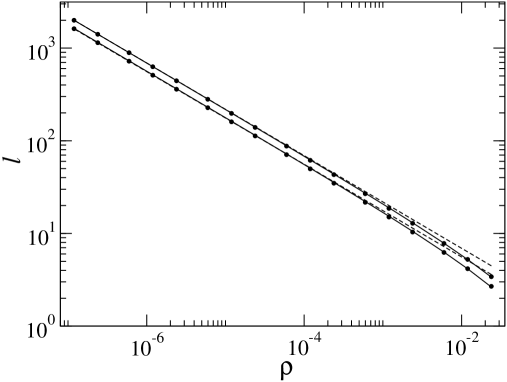
  Figure 2: Plot $\langle|{\bf Y}|\rangle$ (bottom full circles) and $l=\sqrt{\langle{\bf Y}^{2}\rangle}$ (top full circles) obtained from numerical simulations in $D=3$. We compare these data to the functional forms of Eqs. (104,105) (straight dotted lines), finding a good agreement at small density. Note that a very good fit can be obtained in the entire range of density by using the functional form $l_{fit}=l_{theory}-l_{0}$, where $l_{0}\approx 1$, for $a=1$ (full lines).

  In Fig. 3, we plot the numerical probability density distribution $p(r)$ for $\rho=10^{-6}$, which compares very well with our analytical result of Eq. (107).

  

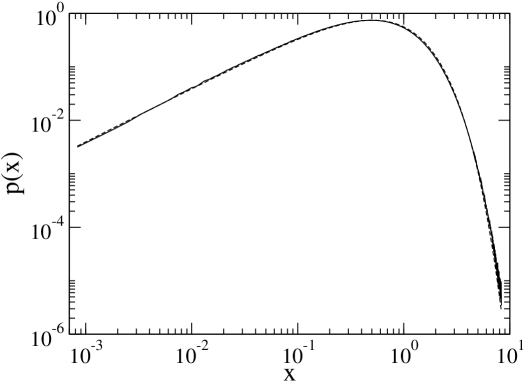
  Figure 3: In three dimensions and for $\rho=10^{-6}$, we plot the numerical probability density distribution of the distance traveled before absorption normalized by its average, $x=Y/\langle Y\rangle$ (full line), obtained after running a total of $2{\times}10^{8}$ random walkers. It is in very good agreement with the theoretical expression of Eq. (107), which leads to $p(x)=4x\exp(-2x)$ (dashed line).

• $D>3$: In higher dimensions, we find the same qualitative behavior as in $D=3$. In particular, the screening length is

  $$l=\sqrt{\frac{2D}{\sigma(D)\rho a^{D-2}}},$$ (108)

  and is amplified by a factor $\sqrt{1+\frac{\kappa}{\lambda a}}$ for imperfect absorbers.

V The case of strongly Correlated absorbers

V.1 Exact result in one dimension

In this section, we consider the case of a non uniform distribution of absorbers displaying long range density-density correlations. In one dimension, such a situation arises naturally when the distribution of intervals $q(L)$ between absorbers decays as a power law up to a distance $\xi$, which is much larger than the mean distance between absorbers $\rho^{-1}$. Hence, we take the typical form

$$q(L)\sim(1-\alpha)\frac{a^{1-\alpha}}{L^{2-\alpha}}\exp(-L/\xi),$$ (109)

for $L$ larger than a small scale cut-off $a$ ($a$ should not be confused with the size of absorbers, which is irrelevant for perfect absorbers in $D=1$; here we consider point-like absorbers). We only consider

$$0<\alpha<1.$$ (110)

The condition $\alpha<1$ ensures that $q(L)$ can be normalized even in the limit $\xi\to\infty$, whereas $\alpha>0$ implies that the first moment diverges in this limit:

$$\langle L\rangle=\rho^{-1}=\frac{1-\alpha}{\alpha}a^{1-\alpha}\xi^{\alpha}.$$ (111)

Since $\alpha<1$, $\xi$ is indeed much larger than the mean distance between absorbers for small $\rho$. If the intervals between absorbers are drawn independently with the distribution $q(L)$, the density correlation function $C(r)=\langle\rho({\bf r})\rho({\bf 0})\rangle$ can be computed exactly, through its Laplace transform $\hat{C}(s)$, which is simply related to the Laplace transform of $q(L)$ by the relation iia

$$\hat{C}(s)=\rho\frac{\hat{q}(s)}{1-\hat{q}(s)}.$$ (112)

Hence in real space, the connected density correlation behaves like

$$\langle\rho({\bf r})\rho({\bf 0})\rangle-\rho^{2}\sim\rho\frac{a^{\alpha-1}}{r^{\alpha}}\exp(-r/\xi).$$ (113)

Now applying the general result of Eq. (84), we obtain

$$l=\sqrt{\frac{\alpha}{6(\alpha+2)}}\,\xi\sim a^{1-1/\alpha}\rho^{-1/\alpha}.$$ (114)

In one dimension, we find that the screening length scales as the correlation length, which is much larger than the screening length obtained in the uniform case. In the next subsections, we shall illustrate the fact that this very same result should apply in higher dimensions.

V.2 A heuristic argument in higher dimensions

We consider a system where the absorbers are distributed via a physical process which leads to long-range spatial correlations between them. Typical examples are given by directed percolation (see next subsection), percolation or DLA, the latter being briefly discussed in section VI. In general, the presence of correlations makes the problem much more difficult to treat analytically. Here, we present a semi-phenomenological approach based on our mean-field renormalization method, which applies in the case where correlations manifest themselves as a clustering phenomena. We define the spatial correlation function as

$$\langle\rho({\bf r})\rho({\bf 0})\rangle=\rho c({\bf r})+\rho^{2},$$ (115)

where the normalized connected correlation function $c({\bf r})$ is assumed to behave qualitatively as

$$c({\bf r})\sim{\exp(-r/\xi)\over r^{\alpha}},$$ (116)

where $\xi$ is the correlation length of the system. We also assume that the system is isotropic. A relationship between the density and $\xi$ is found by associating $\xi$ as the characteristic distance where the connected part of the above correlation function, the first term in Eq. (115), is of the same order as the second term. This gives

$$\rho\sim{\xi^{-\alpha}}.$$ (117)

We implicitly consider the case where $\xi$ is much bigger than the mean distance between absorbers, which scales as $\rho^{-1/D}$. Hence, we will assume from now that

$$\alpha<D.$$ (118)

The regime of small density thus obviously corresponds to a regime where the correlation length is large, for instance near a continuous transition. If the correlation is manifested by the formation of clusters, then the typical number of absorbers in a cluster is given by

$$M_{c}=\int c({\bf r})\,d{\bf r}\sim\xi^{D-\alpha},$$ (119)

which is divergent as $\xi\to\infty$, since $\alpha<D$. If $N_{c}$ is the number of clusters in the volume ${\cal V}$, the total number of absorbers is given by $N\sim N_{c}\xi^{D-\alpha}$, which leads to the cluster density

$$\rho_{c}\sim\rho\,\xi^{\alpha-D}\sim\xi^{-D}.$$ (120)

This last result expresses the fact that the typical distance between clusters of absorbers is of order $\xi$. We thus expect to find large empty regions in the system, whose linear size is of order $\xi$, which is, again, much bigger than the mean distance between absorbers. In what follows, we will repeat our renormalization calculation but in terms of the cluster number. As a starting point, we will use the approximation of Eq. (89), where the potential $V$ is concentrated at the center of the clusters and will take the form

$$V(r)=\lambda{\exp(-r/\xi)\over r^{\alpha}},$$ (121)

which is simply proportional to the mean density of absorbers for a cluster whose center is at $r=0$. For large $\lambda$, the flow equation in $\rho_{c}$ leads to the same functional form for $g$ as before, but the corresponding equation for $s=m^{2}$ is now

$${\partial m^{2}\over\partial\rho_{c}}={\int c(r)r^{D-1}dr\over\int c(r)g(r)r^{D-1}dr}.$$ (122)

We first consider the case $\alpha<2$. In the limit of small $m$ and large $\xi$, we find

$${\partial m^{2}\over\partial\rho_{c}}\sim{\xi^{D-\alpha}(m+\xi^{-1})^{2-\alpha}}\sim{\xi^{D-2}(1+m\xi)^{2-\alpha}},$$ (123)

where we have used $g(r)\sim\exp(-mr)/r^{D-2}$. Using the relation $\rho_{c}\sim\xi^{-D}$, we finally obtain

$$m\xi{\partial m\over\partial\xi^{-1}}\sim(1+m\xi)^{2-\alpha}.$$ (124)

This homogeneous equation admits the obvious solution

$$m\sim{\xi^{-1}},$$ (125)

leading to

$$l\sim\xi\sim a^{1-D/\alpha}\rho^{-1/\alpha},$$ (126)

where we have reintroduced the dependence on the absorber radius $a$.

In the case where $\alpha>2$, the integral in the denominator of the right-hand side of Eq. (122) converges and we simply get

$$m^{2}\sim\rho_{c}\xi^{D-\alpha}\sim\xi^{-\alpha}\sim\rho,$$ (127)

or

$$l\sim a^{1-D/2}\rho^{-1/2},$$ (128)

which is the result for uncorrelated absorbers.

For $\alpha=2$ or $D=2$, the calculation above leads to logarithmic corrections in the expression of $l$. Considering the crudeness of our argument, we do not believe it is worth detailing the nature of these corrections.

In conclusion, the present results suggest that the screening length for a correlated system is either the correlation length $\xi$ ($\alpha<2$) or the screening length found in the uncorrelated case ($\alpha>2$). This result can be expressed in a synthetic way by

$$l\sim\max\left(\xi,a^{1-D/2}\rho^{-1/2}\right),$$ (129)

with logarithmic corrections for the uncorrelated result in $D=2$, which were obtained analytically in section IV.

V.3 Numerical results for a critical distribution of absorbers arising from directed percolation

In this section, we will test the ideas presented above by considering a correlated distribution of absorbers generated by the active sites remaining at time $t$, at the critical point of directed percolation hinri .

Let us briefly introduce directed percolation on a $D$-dimensional hypercubic lattice. Lattice sites are empty (inactive) or occupied by a particle (active). At time $t$, each site is visited in a parallel dynamics. If the site is occupied, the particle is copied on its $2D$ neighbors with probability $p$, or removed with probability $1-p$. If at least one particle has been copied on a given site, this site is simply considered as occupied, and empty otherwise. If $p$ is large enough, a finite stationary density of particles $\rho$ establishes itself for large time. On the contrary, for small enough $p$, the density decays exponentially with time. In fact, there exists a critical value $p_{c}$ for which the system is critical: the density decreases algebraically, and the spatial (and temporal) correlation length diverges with time. This defines the critical exponents $\delta$ and $z$

$$\rho\sim t^{-\delta},\qquad\xi\sim t^{1/z},$$ (130)

and the density correlation function has the typical form introduced in Eq. (115,116), with

$$\alpha=\delta z.$$ (131)

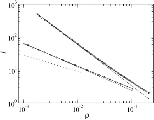
Figure 4: Plot of $l=\sqrt{\langle{\bf Y}^{2}\rangle}$ obtained from numerical simulations of directed percolation in $D=2$ (top dots; 30 samples on a $4000^{2}$ lattice) and $D=3$ (bottom dots; 70 samples on a $300^{3}$ lattice). Each point corresponds to an average over a total of $10^{7}-10^{8}$ random walkers, and error bars are smaller than the size of the dots, except for the smallest densities in $D=2$, where both are of the same order. The dashed lines have the expected slopes $1/\alpha=(\delta z)^{-1}$. In both case, the initial curvature can be well captured by a two-parameter fit to the functional form $l=A\rho^{-1/\alpha}+B\rho^{-1/2}$, where the second term corresponds to the uncorrelated screening length (full lines). Note that the stronger curvature in $D=2$ could as well be due to subleading logarithmic corrections as suggested in subsection V.2. The dotted line represents the slope $-1/2$, which is the expected result in the uncorrelated case, and which holds for $D\geq 4$.

We have performed extensive numerical simulations of directed percolation at the critical point and considered the active sites present at several fixed times. When any of these times is reached, we stop the simulation and launch a large number of random walkers which are absorbed by the active sites. We then measure $\langle|{\bf Y}|\rangle$ and the screening length $l=\sqrt{\langle{\bf Y}^{2}\rangle}$, which are found to be proportional. Finally, the directed percolation dynamics is resumed until the next sampling time is reached, permitting us to explore systems with smaller and smaller densities, and increasing correlation length. We have performed our simulations in $D=2$ and $D=3$, since our $D=1$ result being exact, there is no doubt that the relation $l\sim\xi$ should be satisfied in this case. For $D<4$ ($D_{c}=4$ is the critical dimension above which mean-field theory becomes exact), we have $\alpha<2$. Interestingly, the equality $\alpha=2$ holds exactly in $D=4$ and above ($\delta=1$ and $z=2$), so that for $D\geq 4$, we recover the result $l\sim\rho^{-1/2}$, identical to the uncorrelated case. This is comforting, as correlations are known to become irrelevant above the upper critical dimension. For the dimensions of interest here, one has hinri

$$\alpha_{D=2}\approx 0.79,\qquad\alpha_{D=3}\approx 1.39.$$ (132)

In Fig. 4, we plot $l=\sqrt{\langle{\bf Y}^{2}\rangle}\sim\langle|{\bf Y}|\rangle$ as a function of $\rho$, and find a fair agreement with our prediction $l\sim\rho^{-1/\alpha}$. The numerical data are consistent with a subleading correction of order $\rho^{-1/2}$ (the uncorrelated result), although the rather strong curvature observed in $D=2$ could be as well ascribed to subleading logarithmic corrections mentioned at the end of subsection V.2.

We have also measured the average void size $\lambda$. We pick a point at random in space and determine the radius of the largest disk (in $D=2$) or sphere (in $D=3$) which does not contain any absorber. In $D=1$ (see Eq. (83)), this is exactly a measure of $\xi$ since

$$\lambda=\frac{1}{4}\frac{\langle L^{2}\rangle}{\langle L\rangle}=\frac{3}{4}\langle|Y|\rangle\sim l\sim\xi.$$ (133)

In higher dimension, we expect this property to hold, since $\lambda$ measures the typical distance between absorber clusters, as discussed in subsection V.2, which was found to be of order $\xi$. In fact, we postulate the more general result

$$\lambda\sim\max\left(\xi,\rho^{-1/D}\right).$$ (134)

Fig. 5 illustrates the very convincing linear relation found numerically between $l$ and $\lambda$, implying $l\sim\xi$. Note that we have the obvious bound

$$l>\lambda,$$ (135)

as a particle cannot be absorbed in empty regions.

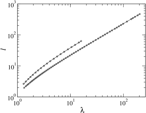
Figure 5: Plot of $l=\sqrt{\langle{\bf Y}^{2}\rangle}$ obtained from numerical simulations of directed percolation in $D=2$ (bottom dots) and $D=3$ (top dots) as a function of the average void size $\lambda$ (see text), which is expected to be an alternative measure of $\xi$. The fits to the linear functional form $l=A\lambda+B$ are excellent (full lines). The curvature is due to our choice of a log-log plot, in order to show that the linear fit works well in the entire range of $\lambda$. Note that $\lambda$ also seems to share the same statistical fluctuations as $\xi$, so that $\xi$ as a function of $\lambda$ in $D=2$ is much smoother than when expressed as a function of $\rho$ (compare with Fig. 4, for very small $\rho$).

V.4 Exact results for some tubular structures in $D\geq 2$

In this section, we consider a specific geometry in $D\geq 2$ where the screening length can be computed exactly, confirming our general result of Eq. (129).

Let us start by describing the model in $D=2$. We consider one dimensional semi-infinite half-lines ($x>0$) of absorbers separated by a distance $L$ drawn independently with the distribution $q(L)$. Random walkers start from $x<0$, and the screening length $l$ is defined as the average depth reached by the walkers before being absorbed. In this context, $l$ can be also viewed as a penetration length, similar to the one defined for DLA (see section VI). A random walker penetrating a channel of width $L$ will be absorbed at a depth of order $L$, the only relevant length scale. Actually, the random walker density $u$ in the tube can be computed exactly, by solving the system

$$\nabla^{2}u=0,$$ (136)

with the absorbing condition for $x>0$

$$u(x,y=0)=u(x,y=L)=0,$$ (137)

and a constant input of walkers at the entrance of the tube

$$u(x=0,0\leq y\leq L)=1.$$ (138)

Using discrete Fourier transform along the direction $y$, we arrive at the result

$$u(x,y)=\frac{4}{\pi}\sum_{n=0}^{+\infty}\frac{1}{2n+1}{\sin\left(\frac{(2n+1)\pi y}{L}\right)}\exp\left(-\frac{(2n+1)\pi x}{L}\right),$$ (139)

which can also be written as a cumbersome expression involving standard $\ln$ and $\arctan$ functions. The flux of particles deposited at the depth $x$ is

$$\phi(x)=2{\partial u\over\partial y}(x,0)=\frac{4}{L\sinh\left(\frac{\pi x}{L}\right)},$$ (140)

which decays exponentially over the scale $L$. The average deposition depth is then

$$l(L)=\int_{0}^{+\infty}\frac{4x\,dx}{L\sinh\left(\frac{\pi x}{L}\right)}=L.$$ (141)

If we have an array of such channels, the probability that a walker first enters a channel of width $L$ is

$$Q(L)={L\over\langle L\rangle}q(L).$$ (142)

If we neglect the process where a random walker leaves this first channel to be absorbed in an other one, we find

$$l=\int_{0}^{+\infty}Q(L)l(L)\,dL=\frac{\langle L^{2}\rangle}{\langle L\rangle},$$ (143)

where $\langle L\rangle$ is the inverse of the absorber density $\rho$. If $q(L)$ decreases rapidly, $\langle L^{2}\rangle\sim\rho^{-2}$, and we find

$$l\sim\rho^{-1}.$$ (144)

In this geometry, the absorbers are highly correlated since they accumulate on lines. Note that the correlation function averaged over angle initially decreases as $r^{-1}$, so that Eq. (144) is fully consistent with our general result for $\alpha=1$. Finally, if the width distribution has a power law decay as in Eq. (109), Eq. (143) leads to

$$l\sim\xi\sim\rho^{-1/\alpha},$$ (145)

again in perfect agreement with our general result.

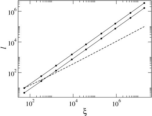
Figure 6: We consider a semi-infinite tubular system in $D=2$ (see text), where the tube width distribution is $q(L)\sim L^{\alpha-2}$, for $L\in[1,\xi]$. For $\alpha=3/4$, we plot $\langle|{\bf Y}|\rangle$ (bottom dots) and $l=\sqrt{\langle{\bf Y}^{2}\rangle}$ (top dots) as a function of the correlation length $\xi$. The fits to the linear functional form $l=A\xi+B$ are excellent (full lines). We also show $\langle L\rangle=\rho^{-1}$ (dashed line), which behaves as $\xi^{\alpha}$, for large $\xi$. Each points is an average over at least $10^{6}$ random walkers, involving a total of $10^{7}$ absorbing tubes, so that the error bars are much smaller than the size of the points.

In Fig. 6, we present numerical simulations of this two-dimensional tubular system. The data are in perfect agreement with Eq. (145), showing that the processes involving particles leaving a tube to be absorbed in an other one do not affect our general result.

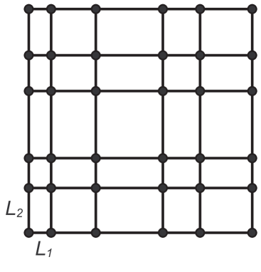
Figure 7: In the tubular model introduced in section V.4, the structure consists of linear tubes whose $(D-1)$-dimensional section is a cross product generated by $D-1$ linear chains. The absorbers lives on the $(D-2)$-dimensional surface of “rectangles” of size $L_{1}{\times}L_{2}{\times}...{\times}L_{D-1}$. The figure shows a view from the top of the structure in $D=3$, where the sections of the tubes are true rectangles. In the model of section V.5, the $D$-dimensional structure is generated by placing the absorbers at the intersection of the product of $D$ linear chains. The figure shows the absorbers (dots) in $D=2$.

This model can be generalized in higher dimensions in the following way. We consider linear tubes whose $(D-1)$-dimensional surface is perfectly absorbing. A $(D-1)$-dimensional cut of the system has the structure of a network of $(D-1)$-dimensional “rectangular” cells of edge length $L_{1}$, $L_{2}$,…, $L_{D-1}$, which are drawn independently using the same probability distribution $q(L)$. The absorbers are placed on the $(D-2)$-dimensional surface of these cells (see Fig. 7). The density of absorbers is still

$$\rho=\langle L\rangle^{-1}.$$ (146)

The solution of the diffusion problem in each tube is simply

$$u(x,y_{1},...,y_{D-1})=\left(\frac{4}{\pi}\right)^{D-1}\sum_{n_{1}...n_{D-1}=0}^{+\infty}\prod_{j=1}^{D-1}\frac{1}{2n_{j}+1}\sin\left(\frac{(2n_{j}+1)\pi y_{j}}{L_{j}}\right)\exp\left(-\pi x\sqrt{\sum_{k=1}^{D-1}\frac{(2n_{k}+1)^{2}}{L_{k}^{2}}}\right),$$ (147)

which decays exponentially on the scale $l({\bf L})$, with

$$l({\bf L})=\min_{j=1,...,D-1}L_{j}$$ (148)

Hence, neglecting again processes where a walker leaves the first tube it enters to be absorbed elsewhere, the average penetration length is

$$l=\langle L\rangle^{-(D-1)}\int_{0}^{+\infty}dL_{min}\,L_{min}^{2}q(L_{min})\left[\int_{L_{min}}^{+\infty}dL\,Lq(L)\right]^{D-2}.$$ (149)

If $q(L)$ decays rapidly for $L\gg\langle L\rangle$, this integral leads to

$$l\sim\langle L\rangle\sim\rho^{-1}.$$ (150)

However, if $q(L)$ takes the form of Eq. (109), we find

$$l \sim \langle L\rangle^{-(D-1)}\int_{0}^{+\infty}dL\,L^{2}L^{\alpha-2}\exp(-L/\xi)\left[L^{\alpha}\exp(-L/\xi)\right]^{D-2},$$ (151)

$$\sim \langle L\rangle^{-(D-1)}\xi^{(D-1)\alpha+1}\sim\xi,$$ (152)

where we have used the fact that $\langle L\rangle\sim\xi^{\alpha}\sim\rho^{-1}$. We again find $l\sim\xi$, in agreement with our general argument for strongly correlated absorbers.

V.5 Exact results for a product distribution of absorbers in $D\geq 2$

In this section, we consider a system for which absorbers are placed at the intersections of the product of $D$ linear chains (see Fig. 7). Each chain has its intervals drawn from the distribution $q(L)$. The density of absorbers reads

$$\rho=\langle L\rangle^{-D}.$$ (153)

If the distribution $q(L)$ decreases rapidly on the scale of $\langle L\rangle$, it is clear that this system will behave similarly to a uniform distribution of absorbers, leading to $l\sim\rho^{-1/2}$. Hence, we assume that the distribution of intervals is of the form

$$q(L)\sim{L^{-2+\alpha/D}}\exp(-L/\xi).$$ (154)

We shall see below that $\alpha<2$ will lead to $l\sim\xi$, whereas the uncorrelated result is recovered for $\alpha>2$. The correlation function can be exactly computed, since the density is the cross product of $D$ independent densities

$$\langle\rho({\bf x})\rho({\bf 0})\rangle=\prod_{i=1}^{D}C(x_{i}),\qquad{\bf x}=(x_{1},...,x_{D}),$$ (155)

where $C(x)$ is the one dimensional correlation function, which can be exactly computed in terms of the Laplace transform of $q(L)$ (see Eq. (112)). After performing an average over angle, the correlation is found to qualitatively behave as

$$\langle\rho({\bf r})\rho({\bf 0})\rangle-\rho^{2}\sim\frac{\rho}{r^{\alpha}}\exp(-r/\xi).$$ (156)

In the present model, the average void size introduced in section V.3 is defined as the radius of the largest hypercube that does not contain any absorbers, averaged over the position of the center of the hypercube. A simple calculation leads to the generalization of Eq. (133). If the center ${\bf x}=(x_{1},...,x_{D})$ ($x_{i}\in[0;L_{i}]$) is drawn randomly in a cell of size $L_{1}{\times}L_{2}{\times}...{\times}L_{D}$ with all $2^{D}$ corners occupied by an absorber, the largest hypercube not containing any absorber has a radius

$$d({\bf x})=\min_{k=1,...,D}\min(x_{k},L_{k}-x_{k}).$$ (157)

In order to simplify our calculation, we replace the actual expression of $d({\bf x})$, by

$$d({\bf x})=\min(x_{k},L_{k}-x_{k}),\qquad L_{k}=\min_{j=1,...,D}L_{j},$$ (158)

which behaves essentially in the same manner as the original expression. Since the average of $d({\bf x})$ over the position ${\bf x}$ of the center is $L_{k}/4$, we finally get

$$\lambda=\frac{1}{4}\langle L\rangle^{-D}\int_{0}^{+\infty}dL_{min}\,L_{min}^{2}q(L_{min})\left[\int_{L_{min}}^{+\infty}dL\,Lq(L)\right]^{D-1}.$$ (159)

Interestingly, Eq. (159) is the same (up to the $1/4$ factor) as the expression obtained for $l$ in the previous subsection (see Eq. (149)), except that $D-1$ is now replaced by $D$. Hence, if $\alpha<2$, we conclude that

$$l>\lambda\sim\xi\sim\rho^{-1/\alpha}.$$ (160)

In fact, our previous results suggest that $l\sim\lambda\sim\xi$ again. Finally, note that in an homogeneous correlated system, Eq. (159) shows that the distribution of the void linear sizes is typically of the form

$$Q(L)\sim\frac{L^{\alpha-1}}{\xi^{\alpha}}\exp(-L/\xi),$$ (161)

which is identical to the void size distribution $Q(L)$ obtained in $D=1$ (see Eq. (79)).

Note that in $D>2$, we can obtain a regime where the correlation length is large compared to the average distance between absorbers, but is still smaller than the uncorrelated screening length,

$$\rho^{-1/D}\ll\xi\ll\rho^{-1/2}.$$ (162)

This regime corresponds to values of $\alpha$ satisfying,

$$2<\alpha<D.$$ (163)

In this case, although there are long-range correlations in the system, our argument of section V.2 predicts that the uncorrelated result $l\sim\rho^{-1/2}\sim\xi^{\alpha/2}$ should hold. In Fig. 8, we measure numerically $l$ as a function of $\xi$ for the model studied in the present section, and in $D=3$. In perfect agreement with our general result of Eq. (129), we find that $l\sim\xi$ for $\alpha=1.5<2$, whereas $l\sim\rho^{-1/2}$ for $\alpha=2.4>2$. Note that in both cases, we find $\lambda\sim\xi\gg\rho^{-1/D}$ (not shown).

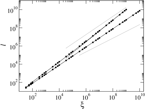
Figure 8: Plot of $l=\sqrt{\langle{\bf Y}^{2}\rangle}$ as a function of $\xi$ obtained from numerical simulations (full circles) for the model where absorbers are placed at the intersections of the cross product of $D$ linear chains in $D=3$. For $\alpha=2.4>2$ (top circles and curves), we find an asymptotic slope $l\sim\xi^{\alpha/2}\sim\rho^{-1/2}$ (top dashed line). The fit to the functional form $l=A\xi^{\alpha/2}+B\xi$ (top full line; where the linear correction corresponds to the correlated result) is excellent. As a guide to the eye, we show the line of slope unity corresponding to the correlated regime $l\sim\xi$ (top dotted line). For $\alpha=1.5<2$ (bottom circles and curves), we find that $l=A\xi$ fits perfectly the data (bottom full line). We also plot a line of slope $\alpha/2=0.75$ (bottom dotted line) to illustrate that $l\sim\xi$ grows much faster than the uncorrelated screening length $\rho^{-1/2}$.

V.6 Temporal decay of the density of random walkers for a correlated density of absorbers

In this subsection, we address the generalization of Eq. (1) for a strongly correlated distribution of absorbers in $D$ dimensions. We shall adapt to the present problem the usual variational argument donsker leading to Eq. (1). Note that the effect of short range clustering on the density of surviving random walkers has been studied quantitatively in new .

Imagine that one releases a random walker of diffusion constant $\kappa$ in an hypercubic region of linear size $L$ not containing any absorber (a void). Its survival probability is larger than the survival probability computed assuming that the boundary of the void is perfectly absorbing. This probability behaves like $P(t)\sim\exp(-\kappa{\bf k}_{L}^{2}t)$, where ${\bf k}_{L}$ is the lowest mode of the diffusion equation in the hypercubic domain delimited by the void, with absorbing boundary conditions on the surface. All the $D$ coordinates of ${\bf k}_{L}$ are equal to $\pi L^{-1}$. By actually solving the diffusion equation mentioned above with a uniform initial position of the random walker, we obtain an exact bound of the form

$$P(t)>\frac{A_{D}}{L^{D}}\exp\left(-\frac{\pi^{2}\kappa Dt}{L^{2}}\right),$$ (164)

where $A_{D}$ is some constant which does not depend on $L$

Finally, and after averaging over the void size distribution $Q(L)$, we find an exact bound for the density of surviving walkers

$$n(t)>A_{D}\int_{0}^{+\infty}Q(L)\exp\left(-\pi^{2}\frac{\kappa Dt}{L^{2}}\right)\,dL.$$ (165)

It is commonly conjectured that this kind of bound actually captures the correct asymptotic behavior of $n(t)$ donsker .

Let us now assume a distribution of hypercubic void sizes of the form found in Eq. (161).

$$Q(L)\sim\frac{L^{\alpha-1}}{\xi^{\alpha}}F(L/\xi).$$ (166)

In $D=1$, or in the preceding section, we considered a cut-off function $F(x)=\exp(-x)$. Here, we will consider the more general case

$$F(x)=\exp(-x^{\gamma}),$$ (167)

where the value $\gamma=D$ is a natural example: $L^{D}/\xi^{D}$ is the volume of the void divided by the correlation volume, an equivalent of the term $\rho L^{D}$ obtained in the usual uncorrelated case (see Eq. (2)).

Dropping all unimportant numerical constants for the sake of clarity, we obtain

$$n(t)\sim\int_{0}^{+\infty}L^{-D-1+\alpha}\exp\left(-\frac{\kappa t}{L^{2}}-\left(\frac{L}{\xi}\right)^{\gamma}\right)\,dL.$$ (168)

Applying a saddle-point argument, and dropping subleading corrections, we finally find that

$$n(t)\sim\exp\left(-C_{D}\left(\frac{\kappa t}{\xi^{2}}\right)^{\frac{\gamma}{\gamma+2}}\right).$$ (169)

We obtain a stretched exponential decay like in the uncorrelated case, but more importantly, we find that the time scale $\tau$ over which the density decays is now controlled by the correlation length

$$\tau=\frac{\xi^{2}}{\kappa},$$ (170)

instead of the density $\rho$, as obtained in the uncorrelated case

$$\tau=\frac{\rho^{-2/D}}{\kappa}.$$ (171)

VI Penetration length for DLA

There have been several attempts to measure the screening length of DLA clusters wit of gyration radius $R$ lintro ; meakin ; llast ; bayard ; locgrowth . In this section, we show that the methods used so far do not effectively measure $l$. We will propose a theoretical estimate for $l$ as well as a possible numerical method in order to measure it properly.

First of all, let us briefly mention how DLA clusters are grown in dimension $D\geq 2$. One first places a seed at the origin, for instance a $D$-dimensional sphere of radius $a$. A random walker (of same radius $a$) is launched from far away and wanders until it touches the seed, whereupon it sticks to it. Then, another random walker is released, which sticks upon contact with any of the quenched particles. This process goes on, leading to the formation of fractal clusters of dimension $D_{f}<D$ (and presumably, $D_{f}>D-1$ wit ), defined as

$$N\sim R^{D_{f}},$$ (172)

where $N$ is the number of particles in the cluster. We immediately note that for an incoming random walker, the points at a distance $2a$ from the already formed structure acts like absorbers. Hence, it is tempting to introduce a screening length $l$ lintro ; meakin , measuring how deep the random walkers penetrate the cluster before sticking to it. However, contrary to the systems studied so far in this paper, which were infinite and homogeneous, a DLA cluster is finite and its density from the center decays in average as

$$\rho(r)\sim r^{-(D-D_{f})}.$$ (173)

The determination of $l$ is an important matter, being often an essential ingredient in the theoretical attempts to determine $D_{f}$. Although mean-field theories are based on contradicting estimates for $l$, typically $l\sim R^{D-D_{f}}$ muka ; mf1 or $l\sim R^{(D-D_{f})/2}$ mf2 , they mostly consider that $l\ll R$. However, there is now convincing numerical evidence meakin ; llast ; bayard showing that

$$l\sim R,$$ (174)

at least in $D=2$, and probably in $D=3$. To understand this result, it is worth mentioning the commonly used method to determine $l$ meakin ; llast . A cluster of large size $R$ is first grown. Then a large number of independent random walkers are released. If one of them touches a particle of the cluster, it simply vanishes, and its last position is recorded. The distribution of the positions of absorption is thus obtained and its standard deviation is considered as a measure of $l$ (before or after averaging over many clusters having the same number of particles). Although a certain consensus seems to exist in the literature, we do not believe that this variance is a faithful measure of $l$. To see this, let us consider the simple example of a perfectly absorbing ellipse in $D=2$ of aspect ratio $e>1$ and main axis $R$. Any method to measure $l$ should retrieve the trivial result that $l=0$ in this case. However, the method presented above would obviously lead to $l\sim R\,$! It is correct that DLA clusters grown in the continuum are statistically isotropic. However, for a given cluster, the fluctuation of the length of the main branches are typically of size $R$, leading to an automatic numerical evaluation of $l\sim R$. In other words, even if the random walkers were only absorbed near the tip of these branches, physically implying a very small value of $l$, the current method of estimating $l$ would invariably lead to $l\sim R$.

As an alternative method (but which might prove as ineffective as the one above), we propose that one should measure the distance of penetration from the convex hull of the cluster, and to measure the variance of this length before averaging over many clusters. At least, this method gives the correct result for the ellipse (its own convex hull), that is, $l=0$.

Finally, inspired by the general conclusions of the previous sections, we would like to give three related arguments in favor of the result $l\sim R$, which we think is correct, although it is argued that the available numerical simulations using the method exposed above are not conclusive on this matter. Particles in a DLA cluster are obviously strongly correlated, arranging themselves in highly ramified structures. It is thus tempting to apply some of our result to this situation:

• There is no finite correlation length in a DLA cluster except, rather trivially, for the size of the cluster itself. For long-range correlations, we have found that $l\sim\xi\sim R$.

• In a DLA cluster, the density correlation function decays as $c(r)\sim r^{-\alpha}$, with $\alpha=D-D_{f}$. Our study suggests that $l\sim\rho^{-1/\alpha}\sim R$ (see Eq. (173)).

• Since a DLA cluster is fractal, the largest voids inside it are of typical linear size $\lambda\sim R$. In homogeneous structures, $l>\lambda$, which suggests again that for DLA, $l\sim R$.

VII Conclusion

In this paper, we have justified analytically the heuristic argument presented in the introduction to estimate the screening length in a system of uniformly distributed perfect or imperfect absorbers. Our results in $D=2$ and $D=3$ are in excellent agreement with numerical simulations. Even the numerical prefactors of the two first moments are surprisingly well described by our approach. As a further check, we found that the theoretical distribution of the distances of absorption is in perfect agreement with numerical simulations.

For correlated absorbers, our analytical approach is not as rigorous as in the uncorrelated case, although we supplemented our heuristic argument with the exact solution in $D=1$ as well as for two toy models in $D>1$, which fully confirm our general results. We find that if the density correlation function decays with an exponent $\alpha$ ($\alpha<2$ in $D\geq 2$, and $\alpha<1$ in $D=1$) up to the correlation length $\xi\sim\rho^{-1/\alpha}$, then the screening length scales as $l\sim\xi\sim\lambda$, where $\lambda$ is the average void linear size. These results were confirmed numerically in directed percolation, where the active sites play the role of the absorbers.

Finally, we have argued that for DLA, the penetration or screening length $l$ should be of the same order as the linear size $R$ of a cluster. We have also emphasized that the current numerical method of determining $l$, although finding just $l\sim R$, could hardly lead to any other result. As a more appropriate method, we propose measuring the distance of penetration from the convex hull of the cluster, and to define $l$ as the standard deviation of this length before averaging over many clusters. With this definition, the behavior of $l$ as a function of the cluster radius $R$ is certainly a question worth investigating unpub .

- (1) B. Ya. Balagurov and V. G. Vaks, Zh. Eksp. Teor. Fiz. 65, 1939 (1973) [Sov. Phys. JETP 38, 968 (1974)]; M. Donsker and S. Varadhan, Commun. Pure Appl. Math. 28, 525 (1975); P. Grassberger and I. Procaccia, J. Chem. Phys. 77, 6281 (1982); T. C. Lubensky, Phys. Rev. A 30, 2657 (1984); S. Renn, Nucl. Phys. B 275, 273 (1986); J. W. Haus and K. W. Kehr, Phys. Rep. 150, 263 (1987); T. M. Nieuwenhuizen, Phys. Rev. Lett. 62, 357 (1989).
- (2) M. Muthukumar, Phys. Rev. Lett. 50, 839 (1983).
- (3) D. S. Dean, I. T. Drummond, R. R. Horgan, and A. Lefèvre, J. Phys. A 37, 10459 (2004).
- (4) C. Itzykson and J.-M. Drouffe, Statistical Field Theory, Volume 1 (Camdridge, 1992).
- (5) W. Feller, An Introduction to Probability Theory and Its Applications, Volume 1 (Wiley, New York, 1957).
- (6) M. Abramowitz and I. A. Stegun, Handbook of mathematical functions (Dover, 1965).
- (7) S. N. Majumdar, C. Sire, A. J. Bray, and S. J. Cornell, Phys. Rev. Lett. 77, 2867 (1996); B. Derrida, V. Hakim, and R. Zeitak, Phys. Rev. Lett. 77, 2871 (1996).
- (8) H. Hinrichsen, Adv. Phys. 49, 815 (2000).
- (9) Yu. A. Makhnovskii, A. M. Berezhkovskii, D.-Y. Yang, S.-Y. Sheu, and S. H. Lin, Phys. Rev. E 61, 6302 (2000).
- (10) T. A. Witten and L. M. Sander, Phys. Rev. Lett. 47, 1400 (1981).
- (11) M. Plischke and Z. Rácz, Phys. Rev. Lett. 53, 415 (1984).
- (12) S. Tolman and P. Meakin, Phys. Rev. A 40, 428 (1989).
- (13) R. C. Ball, N. E. Bowler, L. M. Sander, and E. Somfai, Phys. Rev. E 66, 026109 (2002).
- (14) B. K. Johnson, R. F. Sekerka, and M. P. Foley, Phys. Rev. E 52, 796 (1995).
- (15) J. Lee, S. Schwarzer, A. Coniglio, and H. E. Stanley, Phys. Rev. E 48, 1305 (1993).
- (16) M. Matsushita, K. Honda, H. Toyoki, Y. Hayakawa, and H. Kondo, J. Phys. Soc. Japan 55, 2618 (1988).
- (17) H. G. E. Hentschel, Phys. Rev. Lett. 52, 212 (1984); M. Tokuyama and K. Kawasaki, Phys. Lett. A 100, 337 (1984); K. Ohno, K. Kikuchi, and H. Yasuhara, Phys. Rev. A 46, 3400 (1992).
- (18) J. Sopik, C. Sire, and D. S. Dean, in preparation.