Decoherence in Josephson vortex quantum bits

Abstract

We investigated decoherence of a Josephson vortex quantum bit (qubit) in dissipative and noisy environment. As the Josephson vortex qubit (JVQ) is fabricated by using a long Josephson junction (LJJ), we use the perturbed sine-Gordon equation to describe the phase dynamics representing a two-state system and estimate the effects of quasiparticle dissipation and weakly fluctuating critical and bias currents on the relaxation time $T_{1}$ and on the dephasing time $T_{\phi}$. We show that the critical current fluctuation does not contribute to dephasing of the qubit in the lowest order approximation. Modeling the weak current variation from magnetic field fluctuations in the LJJ by using the Gaussian colored noise with long correlation time, we show that the coherence time $T_{2}$ is limited by the low frequency current noise at very low temperatures. Also, we show that an ultra-long coherence time may be obtained from the JVQ by using experimentally accessible value of physical parameters.

I Introduction

Novel superconducting quantum bits (qubits), such as charge (i.e., Cooper-pair box),charge flux,flux and phase qubits,phase are good candidates for quantum information processing because these can be manufactured, controlled, and scaled more easily. Tens of quantum oscillations had been observed in these qubits, but a low level of decay which yields thousands of coherence oscillations is essential for realization of quantum computation. The longest coherence time of 0.5 $\mu$s has been reported for the quantroniumchfl (i.e., hybrid charge-flux qubit), but longer time may still be necessary. As many decoherence sources reduce the quantum oscillations, the measured value of the coherence time for the superconducting qubits is substantially shorterHar than that predicted by the simplest models of decoherence and that needed for the operation of a quantum computer. This requirement of obtaining ultra-long coherence time in the presence of the interaction between the qubit system and noisy environment is one of major challenges.

Understanding the mechanisms of decoherence became a focus of much attention recently, and it remains an important challenge for the superconducting qubits. An ideal solution is to isolate the qubit system from uncontrolled degree of freedom in its environment and in the device itself. However, it is difficult to isolate the qubit system completely from the decoherence sources. These sources include, but may not be limited to, background charge fluctuations in the substrate,shot fluctuations in the tunnel barrier which produce microscopic tunneling resonance,micro and fluctuating electromagnetic background. Also, low frequency variation in the critical currentHar is present in all superconducting qubits. One way to obtain the ultra-long coherence time is to use the Josephson vortex qubit (JVQ) since it msy be immune to these sources.

Recently, JVQ has been proposed as a new superconducting qubit.Cl This qubit has two important advantages over other superconducting qubits. First, coupling between the qubit system and the decoherence sources is weak at very low temperatures. For example, a Josephson vortex (i.e., fluxon) in a uniform long Josephson junction (LJJ) does not generate any radiation during its motion and is almost decoupled from other electromagnetic excitations in the junction. Also the qubit is immune to fluctuations in the critical current. Consequently, quantum coherence can be maintained much longer than other qubits which are susceptible to these decoherence sources. Second, as the fluxon dynamics in LJJ is described by using the perturbed sine-Gordon equation,MS the decoherence sources for the qubit may be easily identified. For example, two important sources are the quasiparticle dissipation and weak current noise. Hence, the coherence time may be estimated more easily, but the effect of these sources has not yet been estimated for the JVQ.

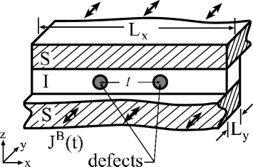
Figure 1: A LJJ stack is shown schematically as alternating layers of superconductors ($S$) and insulator ($I$). $L_{x}$ and $L_{y}$ denote the dimensions in $x-$ and $y-$direction, respectively. $J^{B}(t)$ denotes the time dependent bias current density. The filled dashed circles represent the microresistors which behave as pinning centers for fluxon.

The JVQ exploits the property of fluxon,KI ; Sh which behaves as a quantum particle at ultra-low temperatures. The fluxon trapped in a controllable potential well in a single annular LJJ shows (i) energy quantization in the potential well and (ii) macroscopic quantum tunneling (MQT) from a metastable state.Wa Also, it was shown that the two quantum states for the qubit can be created by using a heart-shapedWa annular LJJ and by trapping a fluxon in a magnetic field-controlled double-well potential. These quantum states may also be created using a linear LJJ with two closely implanted defect sites in the insulator layer.KI A Nb-AlO_x-Nb junction may be used to fabricate the JVQ, as shown schematically in Fig. 1. The dimensions of the junction, compared to the Josephson length $\lambda_{J}$, are $L_{x}\gg\lambda_{J}$ and $L_{y}\ll\lambda_{J}$. The separation distance $\ell$ between the defect sites must be larger than the critical distance $\ell_{o}$, as discussed below. Also, the preparation of initial state and the read-out of the final qubit state may be performed by using classical circuits.KU

As the effect of the decoherence sources in the LJJ is described by using the perturbed sine-Gordon equation, the coherence time $T_{2}$,

$${1\over T_{2}}={1\over 2T_{1}}+{1\over T_{\phi}}~{},$$ (1)

for the JVQ may be estimated without making further assumptions about the nature of the qubit-environment interaction. Here $T_{1}$ is the relaxation time, and $T_{\phi}$ is the dephasing time. Since $T_{\phi}$ is most sensitive to the decoherence sources, extending $T_{\phi}$ for the superconducting qubits is important for quantum computing applications. We compute $T_{2}$ by accounting for the two sources: (i) quasiparticle dissipation and (ii) weak current noise. It is noted that the JVQ may also couple to other sources, such as microwave and phonon radiation, but the effect of these sources is expected to be small as they lead to higher orderIo contribution in the perturbation expansion than that considered in the present paper. In the JVQ, the weak current noise represents the low frequency magnetic field and current fluctuations in the junction. We focus on slow fluctuations since the qubits suffer from the presence of strong low frequency noise sources. The effects of these two decoherence sources have been investigated also for other superconducting qubitsXu and were found to be important.

In this paper, we show that the JVQ can yield ultra-long coherence time because it couples very weakly to noisy environment at low temperatures. Before proceeding further, we outline the main results. i) Starting from the perturbed sine-Gordon equation, we show that the critical current fluctuation does not couple to the JVQ within the lowest order approximation. Consequently, this fluctuation effect does not lead to decoherence of the qubit. ii) We show that $T_{2}$ at ultra-low temperatures is determined by the low frequency current noise since the dissipation effect due to qubit-environment coupling is exponentially small. iii) Using experimentally obtained physical parameters, we show that the effect of this current noise on decoherence is weak in the JVQ. This weak coupling between the JVQ and current noise leads to the coherence time of several tens of microseconds for the JVQ.

We outline the remainder of the paper. In Sec. II, we express the phase dynamics of LJJ in the collective coordinate representation and transform the perturbed sine-Gordon equation onto the double-well potential problem. In Sec. III, we obtain the two-state system, described by the spin-boson model with low frequency current noise. Here, the quasiparticle dissipation is described by using Ohmic environment, and the effects of low frequency noise in LJJ is described by using the fluctuating weak bias current. In Sec. IV, we derive the relaxation time ($T_{1}$) and the dephasing time ($T_{\phi}$) due to these two decoherence sources. In Sec. V, we estimate numerically the coherence time ($T_{2}$) by using the experimentally accessible parameters for LJJ and compare it to that obtained for other superconducting qubits. Finally, in Sec. VI, we summarize the result and conclude.

II long Josephson junction qubit

In this section, we discuss how the LJJ may be used to obtain a JVQ by starting from the perturbed sine-Gordon equation. First, a double-well potential for the fluxon needs to be created in the LJJ to obtain the two quantum states of the JVQ. Several approaches are used to accomplish this. Each of these approaches yields a slightly different form of the potential function. In this paper, we consider the approach of implanting two closely spaced microresistors in the insulator ($I$) layer. When the fluxon does not have enough kinetic energy, the microresistor attracts the fluxon and traps it at the defect site. The effects of quasiparticle dissipation and low frequency weak current noise may be examined by starting with

$${\partial^{2}\varphi\over\partial x^{2}}-{\partial^{2}\varphi\over\partial t^{2}}-\sin\varphi={\cal F}~{},$$ (2)

where $x$ and $t$ are the dimensionless coordinates in units of $\lambda_{J}$ and $\omega_{p}^{-1}$, respectively. Here $\omega_{p}$ denotes the plasma frequency. The dynamic variable $\varphi$ represents the difference between the phase of order parameter for the superconductor ($S$) layers. The perturbation term ${\cal F}=\beta(\partial\varphi/\partial t)-\beta_{s}(\partial^{3}\varphi/\partial t\partial^{2}x)+f(t)+{\bar{\delta J_{c}}}(t)\sin\varphi-\sum_{i}\epsilon_{i}\delta(x-x^{o}_{i})\sin\varphi$ includes the effects due to quasiparticle dissipation ($\beta$ and $\beta_{s}$), bias current ($f=J^{B}/J_{c}$), critical current fluctuation ($\delta{\bar{J}}_{c}(t)=\delta J_{c}(t)/J_{c}$), and microresistors ($\epsilon_{i}=(J_{c}-J^{\prime}_{c})l_{b}/J_{c}\lambda_{J}$). We note that the critical current $J_{c}(t)$ may be expressed as the sum of uniform ($J_{c}$) and weak fluctuation parts ($\delta J_{c}(t)$): $J_{c}(t)=J_{c}+\delta J_{c}(t)$. Here $x^{o}_{i}$, $J^{B}$, $J^{\prime}_{c}$, and $l_{b}$ ($\ll\lambda_{J}$) denote, respectively, the position of inhomogeneity in the $I$ layer, the bias current density, the modified critical current density at the defect site, and the length of the LJJ in which $J_{c}$ is modified. In the discussion below, we neglect the term $\beta_{s}(\partial^{3}\varphi/\partial t\partial^{2}x)$ due to the quasiparticle (surface) current along the junction layer, for simplicity, since both $\beta(\partial\varphi/\partial t)$ and $\beta_{s}(\partial^{3}\varphi/\partial t\partial^{2}x)$ terms yield similar dissipation effects.

The perturbation term $\cal F$ in Eq. (2) is small, and consequently, it does not change the form of the kink within the framework of the lowest approximation.MS We describe the motion of the fluxon in terms of the center coordinates $q(t)$, which are obtained by neglecting $\cal F$. In the absence of the perturbation terms (${\cal F}=0$), the fluxon solution to Eq. (2) in the non-relativistic limit (i.e., $v\ll 1$) is given by

$$\varphi(x,t)\approx 4\tan^{-1}\left[e^{\gamma(v)[x-q(t)]}\right]~{},$$ (3)

where $\gamma^{-1}(v)=\sqrt{1-v^{2}}$, $q(t)=vt$ denotes the center coordinate of the fluxon, and $v$ is the fluxon speed in units of Swihart velocity $c$. $q(t)$ is also known as collective coordinate and represents a dynamical variable. We note that this solution represents propagation of nonlinear wave as a ballistic particle and that the perturbation terms in ${\cal F}$ only affect dynamics of the center coordinates.

Applying the kink solution of Eq. (3) to Eq. (2) for carrying out the classical perturbation theory within the framework of lowest order approximation,MS we obtain the equation of motion for the center coordinate $q(t)$ in the nonrelativistic limit as

$$M{d^{2}q(t)\over dt^{2}}+\beta M{dq(t)\over dt}+{\partial V(q)\over\partial q}=0~{}.$$ (4)

Here $M=8$ denotes the rest mass of the fluxon which is obtained by inserting the waveform of Eq. (3) into the Hamiltonian corresponding to the unperturbed sine-Gordon equation (i.e., Eq. (2) with ${\cal F}=0$).MS $V(q)$ is the effective potential for the fluxon due to the non-dissipative perturbation terms in ${\cal F}$.

The phase dynamics in the center coordinate may be seen easily from the Euclidean Lagrangian, ${\cal L}={\cal L}_{o}+{\cal L}_{P}$ where ${\cal L}_{o}$ and ${\cal L}_{P}$ describes the unperturbed phase dynamic of LJJ and the perturbation contribution, respectively. The unperturbed part of the Lagrangian ${\cal L}_{o}$ is given by ${\cal L}_{o}=\int(dx/2)[(\partial\varphi/\partial\tau)^{2}+(\partial\varphi/\partial x)^{2}+2(1-\cos\varphi)]$. The perturbation part of the Lagrangian ${\cal L}_{P}={\cal L}_{nd}+{\cal L}_{d}$ can be expressed as the sum of the non-dissipative part (${\cal L}_{nd}$) due to the bias current, critical current fluctuation and inhomogeneities, and the quasiparticle dissipation part (${\cal L}_{d}$). The non-dissipative contribution may be expressed as ${\cal L}_{nd}={\cal L}_{bias}+{\cal L}_{\delta J_{c}}+{\cal L}_{pin}$. Here ${\cal L}_{bias}=\int dxf\varphi$, ${\cal L}_{\delta J_{c}}={\bar{\delta J_{c}}}(\tau)\int dx(1-\cos\varphi)$, and

$${\cal L}_{pin}=\sum_{i=1}^{2}\int dx~{}\epsilon_{i}\delta(x-x_{i}^{o})(1-\cos\varphi)$$ (5)

are the Lagrangian for the bias current, critical current fluctuation, and two defect sites, respectively. Following Caldeira and Leggett,CL we account for the quasiparticle dissipation (i.e., $\beta$) by representing the environment as a heat bath. The heat bath may be described as a reservoir of harmonic oscillators with generalized momenta $P_{i}$ and coordinates $Q_{i}$. The dissipation effect due to coupling between the phase variables $\varphi$ and the heat bath is described as

$${\cal L}_{d}=\int dx\sum_{i}\left[{P_{i}^{2}\over 2m_{i}}+{m_{i}\omega_{i}^{2}\over 2}\left(Q_{i}-{c_{i}\varphi\over m_{i}\omega_{i}^{2}}\right)^{2}\right]~{}.$$ (6)

Here, the heat bath parameters $m_{i}$, $\omega_{i}$ and $c_{i}$ characterize the reservoir’s spectral function $J_{\beta}(\omega)$, which is written as

$$J_{\beta}(\omega)={\pi\over 2}\sum_{i}{c_{i}^{2}\over m_{i}\omega_{i}}~{}\delta(\omega-\omega_{i})=\beta\omega~{}.$$ (7)

This spectral function reproduces the dissipation term in Eq. (4) when the heat bath degrees of freedom are integrated out.

We describe the fluxon dynamics by using semiclassical theory as usually doneGJS and by reexpressing the partition function, ${\cal Z}=\int{\cal D}[\varphi]\exp\{-S[\varphi]\}$, with $S[\varphi]=\int d\tau{\cal L}$, in terms of the collective coordinates $q(t)$ as ${\cal Z}=\int{\cal D}[q]\exp\{-S[q]\}$. We take the perturbation expansion in terms of $\beta$, $f$, $\bar{\delta J_{c}}$ and $\epsilon_{i}$, assuming that all of these parameters are small. The lowest order contribution from this expansion is obtained by substituting the soliton solution of Eq. (3) to the action $S[\varphi]$ since the perturbation term $\cal F$ does not modify the soliton waveform in the lowest order.MS ; GJS In this center coordinate representation, the bias current contribution to the action (i.e., $S_{bias}[\varphi]=\int d\tau{\cal L}_{bias}$) yieldsKI

$$S_{bias}[q]=S_{bias}[\varphi(x-q)]-S_{bias}[\varphi(x)]=-\int d\tau(2\pi fq)~{}.$$ (8)

Here the constant $S_{bias}[\varphi(x)]$ is subtracted since we have chosen the origin of potential energy for the center coordinate at $q=0$. On the other hand, the critical current fluctuation contribution (i.e., $S_{\delta J_{c}}=\int d\tau{\cal L}_{\delta J_{c}}$) becomes

$$S_{\delta J_{c}}[q]=S_{\delta J_{c}}[\varphi(x-q)]=S_{\delta J_{c}}[\varphi(x)]~{},$$ (9)

indicating that $S_{\delta J_{c}}[q]$ is independent of $q$. This suggests that the critical current fluctuations do not modify the fluxon potential. Within the lowest order approximation, the low frequency noise corresponding to the critical current fluctuation does not couple to the JVQ, and it does not contribute to decoherence. Also, other perturbation contributions $S_{pin}=\int d\tau{\cal L}_{pin}$ and $S_{d}=\int d\tau{\cal L}_{d}$ can be expressed in the $q$ representation. Combining these perturbation contributions, we may express the partition function as ${\cal Z}=\int{\cal D}[q(\tau)]\exp\{-S_{eff}[q(\tau)]\}$, where the effective action $S_{eff}[q]$ is given by

$$S_{eff}[q]=\int d\tau\left[{1\over 2}M{\dot{q}}^{2}+V(q)\right]~{}~{}~{}~{}~{}$$

$$+{M\over 2}\int d\tau\int d\tau^{\prime}{\cal K}(\tau-\tau^{\prime})[q(\tau)-q(\tau^{\prime})]^{2}~{}.$$ (10)

The quasiparticle dissipation effect (i.e., $\beta$) at the finite temperature $T$ is described by the kernel ${\cal K}(\tau)$

$${\cal K}(\tau)={1\over\pi}\int_{0}^{\infty}d\omega~{}J_{\beta}(\omega)~{}{\cosh(\omega/2T-\omega|\tau|)\over\sinh(\omega/2T)}~{}.$$ (11)

Here we set $\hbar=k_{B}=c=1$ for convenience. The potential function $V(q)$ for the fluxon in the collective coordinates is given by

$$V(q)=-2\pi f(t)q-{2\epsilon_{1}\over\cosh^{2}\left(q-{\ell\over 2}\right)}-{2\epsilon_{2}\over\cosh^{2}\left(q+{\ell\over 2}\right)}~{},$$ (12)

where $\ell$ is the separation distance between two defect sites, as shown in Fig. 1. The fluxon potential $V(q)$ includes the potential tilting effect of the bias current ($f$) and the pinning effect ($\epsilon_{i}$) of the two defect sites.

Figure 2: A double-well potential due to two microresistors is schematically shown for (a) $\epsilon_{1}=\epsilon_{2}=\epsilon$ (symmetric) and (b) $\epsilon_{1}\neq\epsilon_{2}$ (asymmetric). The potential barrier and the oscillation frequency at the stable minimum are denoted by $V_{o}$ and $\omega_{o}$, respectively. Here $f(t)$ is set to zero.

The potential function $V(q)$ of Eq. (12) for $f(t)=0$ has two noteworthy features: (i) finite number of bound states, and (ii) double-well structure. For physical values of $\epsilon_{i}$, at most, several states may be trapped by the fluxon potential. This can be seen easily from the energy eigenstate of the trapped fluxon via a single microresistor,LL which is given by

$${\cal E}_{n}=-{1\over 64}\left[-(1+2n)+\sqrt{1+128\epsilon}~{}\right]^{2}$$ (13)

where $n=0,1,2,\cdot\cdot\cdot$. For $\epsilon=0.27$, only $n=$0, 1, and 2 states, corresponding to the eigenstate energy ${\cal E}_{0}=$-0.383, ${\cal E}_{1}=$-0.136, and ${\cal E}_{2}=$-0.0142, respectively, are bounded by the potential. Also, the double-well structure can be seen easily by setting $\epsilon_{1}=\epsilon_{2}=\epsilon$ (i.e., symmetric double-well) (see Fig. 2(a)) and by expanding the function $V(q)$ about the critical separation distance $\ell_{o}$. We note that a small asymmetry (or bias) of ${\bar{\epsilon}}\approx 8q_{o}\delta\epsilon$ may be easily introduced, as shown in Fig. 2(b), since the critical current $J^{\prime}_{c}$ at the each microresistor is slightly different. This yields a small variation in $\epsilon_{i}$ between the two defect sites (i.e., $|\epsilon_{1}-\epsilon_{2}|=\delta\epsilon$ and $\delta\epsilon\ll 1$). The symmetric potential $V(q)$ shown in Fig. 2(a) has the single-well structure for $\ell<\ell_{o}=\ln[(\sqrt{3}+1)/(\sqrt{3}-1)]\approx 1.317$, but it has the double-well structure for $\ell>\ell_{o}$. For $\ell=\ell_{o}+a$, with $a\ll 1$, the fluxon potential $V(q)$ may be expanded around $q=0$ to obtain

$$V(q)-V(0)\approx-{16\epsilon\over 3\sqrt{3}}aq^{2}+{32\epsilon\over 27}q^{4}~{}.$$ (14)

The potential function of Eq. (14) has the stable states at $q=\pm q_{o}/2$ with $q_{o}=3[a/\sqrt{3}]^{1/2}$. The barrier height $V_{o}$ between two stable states is $V_{o}=2\epsilon a^{2}$ and the frequency $\omega_{o}$ of small oscillation around the stable minimum is $\omega_{o}=\sqrt{(d^{2}V(q)/dq^{2})/M}=(8\epsilon a/3\sqrt{3})^{1/2}$, indicating that $\omega_{o}\gg V_{o}$. This suggests that the JVQ cannot be obtained by placing two microresistors too closely (i.e., $\ell\approx\ell_{o}$) since the potential barrier $V_{o}$ may not be strong enough to localize the fluxon to either well. Hence a larger separation distance $\ell$ is needed to localize the bound states in either potential well.

Figure 3: Dependance of the barrier potential $V_{o}$ (dashed line) and the frequency of small oscillations $\omega_{o}$ (solid line) for the symmetric double-well potential on the separation distance $\ell$ between the two defect sites is schematically illustrated for a) $\epsilon<\epsilon_{c}$ and b) $\epsilon>\epsilon_{c}$. The critical pinning strength $\epsilon_{c}$ is 0.125.

The barrier potential $V_{o}$ must be larger than $\omega_{o}$ in order to obtain a localized ground state in either well without mixing it with the excited state of the system. As $\ell$ increases from $\ell_{o}$, the value of both $V_{o}$ and $\omega_{o}$ increases, but this increase depends on $\epsilon$. As $\ell\rightarrow\infty$, $V_{o}$ approaches $2\epsilon$ while $\omega_{o}$ approaches $\sqrt{\epsilon/2}$. This indicates that, when $\epsilon$ is less than the critical value $\epsilon_{c}$ (i.e., $\epsilon<\epsilon_{c}$), $V_{o}$ remains smaller than $\omega_{o}$ for all $\ell$. However, when $\epsilon>\epsilon_{c}$, $V_{o}$ becomes larger than $\omega_{o}$ as $\ell$ is increased, as shown schematically in Fig. 3. We estimate $\epsilon_{c}=0.125$, assuming that $\omega_{o}(\epsilon_{c})=V_{o}(\epsilon_{c})$ at $\ell=\infty$. We will consider $\epsilon>\epsilon_{c}$ in the discussion below, so that $V_{o}\geq\omega_{o}$.

For the fluxon localized at either left or right side of the symmetric double-well shown in Fig. 2(a), the energy of the ground state is degenerate. We use eigenstates $|R\rangle$ and $|L\rangle$ of the operator ${\hat{\sigma}}_{z}$ with eigenvalues +1 and -1 to represent the right-localized and left-localized state, respectively. These two states are exploited in the JVQ. To do this, we need to ensure that the tunneling rate between the two wells does not mix the ground state with the excited states.

The fluxon in the ground state of the symmetric double-well potential can tunnel from the left side to the right side (and vice versa). This MQT yields splitting of two degenerate fluxon ground states. Within the semiclassical WKB approximation,Lang the tunneling rate $\Delta$ is given by

$$\Delta={\cal A}(0)~{}e^{-{\cal B}(0)}~{},$$ (15)

where

$${\cal A}(0) = \left({8\omega_{o}^{3}q_{o}^{2}\over\pi}\right)^{1\over 2}~{}e^{2\int_{0}^{q_{o}\over 2}dq\left[{\omega_{o}\over\sqrt{{\bar{V}}(q)}}-{1\over q_{o}-2q}\right]}~{},$$ (16)

$${\cal B}(0) = 4\int_{-{q_{o}\over 2}}^{q_{o}\over 2}dq~{}\sqrt{{\bar{V}}(q)}~{},$$ (17)

and ${\bar{V}}(q)=V(q)-V(\pm q_{o}/2)$ denotes the potential energy measured from the bottom of the well. The MQT in the real space represents particle-like collective excitation, reflecting the behavior of the fluxon as a quantum particle. The computed tunneling rate, using the WKB approximation, yields good agreement with the quantum result when many states are bounded by the double-well potential, but this agreement is poor when only the ground state is bounded. In Fig. 4, we compare the result of the semiclassical WKB calculation using Eqs. (15)-(17) and the quantum mechanical calculation to illustrate this difference. The difference between these two results is noteworthy: the WKB calculation overestimates $\Delta$. This difference is large when $\ell$ is small (i.e., small $V_{o}$) but decreases with increasing $\ell$ (i.e., increasing $V_{o}$). We will use the quantum result for $\Delta$ in the discussion below since the coherence time depends on $\Delta$.

Figure 4: The splitting $\Delta$ of the ground state for $\epsilon=0.27$ is plotted to compare the results obtained from the WKB approximation and that obtained from the quantum mechanical calculation.

Numerical solution of the bound state energy for the potential of Eq. (12) (with $f(t)=0$) indicates that the ground state is localized at the either side of the double-well for only limited value of $\ell$, as shown in Fig. 5. The lower and upper shaded areas in Fig. 5 represent the regions in the ($\epsilon$, $\ell$) parameter space where the tunneling rate between the two degenerate ground states and the excited states, respectively, are large so that these states cannot be localized in either well. For a fixed $\epsilon$, the number of localized states in either well increases with $\ell$. This indicates that the separation distance $\ell$ and the pinning strength $\epsilon$ may be chosen so that only the ground state is localized in either well. The parameters which yield localization of only the ground state (i.e., between two shaded regions) may be ideal for obtaining the JVQ.

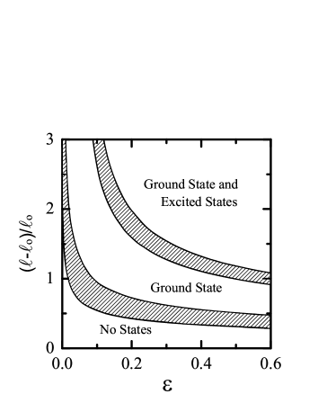
Figure 5: The diagram in the $(\ell,\epsilon)$ parameter space illustrating that bound fluxon states localized in either side of the double-well potential. The shaded areas represent the region with large tunneling rate.

III spin-boson model

In this section, we describe the interaction between the JVQ and noisy environment. We proceed by describing the fluxon dynamics of Eq. (10) in terms of the well-known spin-boson model. This may be carried out by using the two-dimensional Hilbert space spanned by the two degenerate ground states: the fluxon localized at the left well (i.e., $|L\rangle$ ) and at the right well (i.e., $|R\rangle$ ). Following earlier studies, we consider the parameter regime of $V_{o}\geq\omega_{o}\gg\Delta,{\bar{\epsilon}},T$ and include the effects of quasiparticle dissipation and fluctuating weak bias current in the spin-boson model.Legg ; Weiss The Hamiltonian for this model is written as

$$H=H_{S}+H_{SB}+H_{B}~{}.$$ (18)

The spin (S) Hamiltonian $H_{S}$,

$$H_{S}=-{1\over 2}\Delta{\hat{\sigma}}_{x}-{1\over 2}[{\bar{\epsilon}}+{\bar{f}}(t)]{\hat{\sigma}}_{z}~{},$$ (19)

describes the two-state qubit system, which is obtained from the double-well potential of Eq. (12). Here $\Delta$ is the tunneling rate between the two wells. The Pauli operators, ${\hat{\sigma}}_{z}$ and ${\hat{\sigma}}_{x}$, in Eq. (19) represent

$${\hat{\sigma}}_{z}=|R\rangle\langle R|-|L\rangle\langle L|~{},$$ (20)

and

$${\hat{\sigma}}_{x}=|R\rangle\langle L|+|L\rangle\langle R|~{},$$ (21)

respectively. The Hamiltonian $H_{S}$ also accounts for a modification of the simple two-state system by a small asymmetry in the potential due to slight variation in the pinning strength of the microresistors (i.e., $\epsilon_{1}\neq\epsilon_{2}$) and by fluctuating bias current (i.e., $f(t)$). The bias current density ${\bar{f}}(t)=q_{o}f(t)$, representing the driving force for the fluxon, consists of two parts

$$f(t)=f_{o}+\delta f(t)~{},$$ (22)

where $f_{o}$ and $\delta f(t)$ denote the homogeneous and randomly fluctuating weak bias current components, respectively. Here $\delta f(t)$ accounts for the current noise in the JVQ. The Ohmic environment,CL which accounts for the quasiparticle dissipation, is described by the bath (B) Hamiltonian $H_{B}$,

$$H_{B}={1\over 2}\sum_{i=1}^{N}\left({P_{i}^{2}\over m_{i}}+m_{i}\omega_{i}^{2}Q_{i}^{2}\right)~{}.$$ (23)

The interaction between the qubit system and the dissipative environment is described by the spin-bath (SB) Hamiltonian $H_{SB}$,

$$H_{SB}=-{\hat{\sigma}}_{z}{q_{o}\over 2}\sum_{i=1}^{N}c_{i}Q_{i}~{}.$$ (24)

It is noted that the spin-boson model of Eqs. (18), (19), (23), and (24) neglects the contributions from the excited states that are bounded by the potential well. Hence, thermally activated leakage,leak which may also contribute to decoherence at finite $T$, is not accounted in this work. However, we may, safely, assume that this contribution is negligible at ultra-low temperatures. Consequently, the weakly fluctuating bias current (i.e., current noise) at low frequency is the dominant source for dephasing at these temperatures.

We now discuss the time dependent bias current $f(t)$ of Eq. (22). We set the externally applied homogeneous component of the bias current to zero (i.e., $f_{o}=0$) since it yields unwanted asymmetry in the double-well potential (see Fig. 2(b)) for the fluxon. The weak bias current fluctuation ($\delta f(t)$), representing random force in the LJJ due to nonequilibrium states, yields small time-dependent asymmetry in the double-well potential. This asymmetry may be made small but cannot be turned off completely as it arises from the noise-producing environment. This current noise leads the basis states $\{|L\rangle,|R\rangle\}$ to fluctuate weakly, as shown schematically in Fig. 6. However, this effect on the basis state in the JVQ is expected to be smaller than that in other superconducting qubits since the bias current is not used to control the qubit state. It is noted that the effect of noise in the bias current for $f_{o}\not=0$ has been investigated for the phase qubitMar and for the charge qubit.Wei In these qubits, the bias current (i.e., $f_{o}$) is used to control the qubit. Noise in the bias current (i.e., $\delta f$) affects the coherence time of the qubit since it leads to the fluctuation of the qubit state. The bias current noise leads to phase noise for the phase qubitMar and radiation noise for the charge quibit.Wei

To model the effect of this random force more realistically in the JVQ, we describe the bias current fluctuation as Gaussian colored noise with non-zero characteristic correlation time $\tau_{n}$. The current noise $\delta f(t)$ has two main effects on the dynamics of qubit density matrix: i) it leads to transition between two energy eigenstates, and ii) it suppresses coherence between the eigenstates by contributing to pure dephasing. The Gaussian colored noise can be used to account for the noise spectrum with pronounced frequency dependence, such as Lorentzian noise and low frequency asymmetrical magnetic field fluctuationsMC in the tunnel junction. The characteristics of the bias current are described as

$$\langle\delta f(t)\rangle=0~{},$$ (25)

and

$$\langle\delta f(t)~{}\delta f(t^{\prime})\rangle=n_{o}^{2}~{}e^{-|t-t^{\prime}|/\tau_{n}}~{}.$$ (26)

Here $\langle\cdot\cdot\cdot\rangle$ denotes average over different realizations of the fluctuating current, and $n_{o}$ is the typical noise amplitude. We note that, as $\tau_{n}\rightarrow 0$, the colored noise of Eq. (26) becomes the white noise, which is characterized by the correlation function $\langle\delta f(t)~{}\delta f(t^{\prime})\rangle=n_{o}^{2}\delta(t-t^{\prime})$. The correlation function of Eq. (26) indicates that the effects of the current noise for $t\ll\tau_{n}$ differ from those for $t\gg\tau_{n}$. For $t\ll\tau_{n}$, decay of coherence arises from averaging over the distribution of current noise since the fluctuations appear static. For $t\gg\tau_{n}$, on the other hand, decay of coherence is expected to be exponential since the fluctuating bias current behaves as white noise. The crossover behavior occurs at $t\simeq\tau_{n}$. The spectral density of the bias current noise can be taken as

$$S_{noise}(\omega)={2n_{o}^{2}\tau_{n}\over 1+(\omega\tau_{n})^{2}}~{}.$$ (27)

The Lorentzian spectrum of Eq. (27), characterizing telegraph (diachotomous) noise, was observed in intrinsic LJJ.IJJ We note that the noise spectrum in a small tunnel junction is described by the Lorentzian function of Eq. (27), but the $1/\omega$-like noise spectrum in a larger junction may be obtained as a result of several superimposed Lorentzian features.noise In the discussion below, we make few assumptions about the correlation function of Eq. (26): the fluctuation is weak and has small characteristic amplitude (i.e., $n_{o}\ll\Delta$), but it has a long correlation time (i.e., $\tau_{n}\gg 1/\Delta$). Also, we assume that the temperature ($T$) of the bias current producing environment is larger than the cutoff frequency of $1/\tau_{n}$ (i.e., $T\gg 1/\tau_{n}$).

Figure 6: A schematic diagram illustrating the effect of colored noise on the bounded ground state of Josephson vortex in the symmetric double-well potential.

IV decoherence due to fluctuating weak bias current in Ohmic environment

We now discuss the effect of dissipation and noisy environment on the coherence time of the JVQ by using well-established formalism. Here the coherence time represents the time scale for decay of macroscopic quantum coherence (MQC) between the ground states in the double-well potential. Here MQC is due to quantum tunneling of the fluxon which leads to coherent oscillations. This MQC is suppressed by the two decoherence sources since the interaction between the qubit system and its environment can easily destroy the phase coherence between two states. In estimating $T_{2}$, we follow the standard theoretical approach of using the Bloch-Redfield theory and making lowest order Born approximation. The effects of these two sources may be characterized as follows. The Ohmic environment yields the finite relaxation time ($T_{1}$) and dephasing time ($T_{\phi}^{B}$). However, the fluctuating weak bias current modifies $T^{B}_{\phi}$ without significantly changing $T_{1}$. We estimate the effects of the bias current noise, restricting our consideration to $t\gg\tau_{n}$ since the bias current fluctuation appears as $\delta$-function correlated (i.e., white noise), and the quantum coherence decays exponentially. Hence $T_{\phi}$ may be expressed simply as

$${1\over T_{\phi}}={1\over T^{B}_{\phi}}+{1\over T^{noise}_{\phi}}$$ (28)

where $T^{noise}_{\phi}$ is the dephasing time due to weak bias current noise. This indicates that the divergence in $T_{\phi}^{B}$ at ultra-low temperature may be cut off by $T_{\phi}^{noise}$. The contributions from the higher-order Born correction and non-Markovian effect, which are not included in the present work, are small but yield power-law decay.power These contributions may also cut off the diverging $T^{B}_{\phi}$ due to significantly reduced interaction between the qubit system and environment at ultra-low temperatures.

The decay of coherent oscillations is estimated by considering the generalized master equation for the system’s density matrix $\rho_{S}(t)$,

$${d\rho_{S}(t)\over dt}=-i[H_{S},\rho_{S}(t)]-i\int_{0}^{t}dt^{\prime}\Sigma_{S}(t-t^{\prime})\rho_{S}(t^{\prime})~{},$$ (29)

and by assuming that the time dependence of the decoherence source is weak. Here $\rho_{S}(t)={\rm Tr}_{B}\rho(t)$, $\rho=\rho_{S}\bigotimes\rho_{B}$, the kernel $\Sigma_{S}(t)$ is the self-energy operator

$$\Sigma_{S}(t)=-i{\rm Tr}_{B}{\cal H}_{SB}e^{-{\cal QH}t}{\cal H}_{SB}~{}\rho_{B}~{},$$ (30)

${\cal H}_{SB}$ is the Liouvillian superoperator defined by ${\cal H}_{SB}~{}\rho=[H_{SB},\rho]$, and ${\cal Q}=1-\rho_{B}{\rm Tr}_{B}$ is the projection superoperator. Here $\rho_{B}$ is the bath density matrix. Since the studiesHart indicate that both Bloch-Redfield theory and path integral theory yield equivalent results, we employ the former approach for convenience.

The generalized master equation within the Born approximation is obtained by using the fact that the coupling between the qubit system and environment, as described by $J_{\beta}(\omega)/\omega\propto\beta$, is small at low temperatures. We follow the Redfield theoryredfield and make a systematic perturbation expansion of the kernel $\Sigma_{S}$ in powers of the system-bath coupling ($\beta$). We retain only the lowest order terms in this expansion. Replacing $e^{-i{\cal QH}t}\rightarrow e^{-i{(\cal H}_{S}+{\cal H}_{B})t}$ and keeping the expansion of the kernel $\Sigma_{S}$ up to the second order in $H_{SB}$, we obtain

$$\Sigma_{S}^{(2)}(t)=-i{\rm Tr}_{B}~{}{\cal H}_{SB}e^{-i({\cal H}_{S}+{\cal H}_{B})t}{\cal H}_{SB}~{}\rho_{B}~{}.$$ (31)

Further simplification of Eq. (29) may be made by assuming Markov system dynamics

$$\rho_{S}(t-\tau_{o})\sim e^{i{\cal H}_{S}\tau_{o}}~{}\rho_{S}(t)~{},$$ (32)

in which the temporal correlation time $\tau_{o}$ in the dissipative environment is very short due to very short-lived system-bath interactions, and the bath correlation function decays to zero at a very short-time.

Bloch-Redfield equation: In examining the decoherence effects, the Hilbert space spanned by the ground states of the two wells (Fig. 2(a)) is not convenient since the spin Hamiltonian of Eq. (19) is not diagonal in the basis $\{|L\rangle,|R\rangle\}$. We represent the two-state system in new basis $\{|0\rangle,|1\rangle\}$ given by

$$|0\rangle = -|L\rangle\sin\theta+|R\rangle\cos\theta~{},$$ (33)

$$|1\rangle = ~{}~{}|L\rangle\cos\theta+|R\rangle\sin\theta~{},$$ (34)

where $\sin\theta=\sqrt{(\Omega-{\bar{\epsilon}})/\Omega}/\sqrt{2}$, $\cos\theta=\sqrt{(\Omega+{\bar{\epsilon}})/\Omega}/\sqrt{2}$, and $\Omega=\sqrt{{\bar{\epsilon}}^{2}+\Delta^{2}}$. In this new basis $\{|0\rangle,|1\rangle\}$, we estimate $T_{2}$ by making the Born-Markov approximation and by obtaining the Bloch-Redfield equations. Taking matrix elements in the eigenbasis $|n\rangle$ of $H_{S}$ (i.e., $|0\rangle$ and $|1\rangle$), we may write the Redfield equations as

$${d\rho_{nm}^{S}(t)\over dt}=-iE_{nm}~{}\rho_{nm}^{S}(t)-\sum_{kl}{\cal R}_{nmkl}~{}\rho_{kl}^{S}(t)~{},$$ (35)

where $\rho_{nm}^{S}=\langle n|\rho_{S}|m\rangle$, ${\cal R}_{nmkl}$ is the Redfield tensor, $E_{nm}=E_{n}-E_{m}$, and $E_{n}$ is the eigenstate energy of $H_{S}$ (i.e., $H_{S}|n\rangle=E_{n}|n\rangle$). In the absence of the fluctuating bias current ($\delta f$), the eigenstate energies in the diagonal basis, representing the ground state splitting, are expressed as

$$E_{0} = -{1\over 2}\sqrt{{\bar{\epsilon}}^{2}+\Delta^{2}}~{},$$ (36)

$$E_{1} = +{1\over 2}\sqrt{{\bar{\epsilon}}^{2}+\Delta^{2}}~{}.$$ (37)

In the presence of the low frequency bias current fluctuations, these energies fluctuate slowly as shown schematically in Fig. 6. We assume that the eigenstate energies are almost constant in the time scale relevant for the evolution of the density matrix.

The Redfield tensor ${\cal R}_{nmkl}$ is defined by

$${\cal R}_{nmkl}=~{}~{}~{}~{}~{}~{}~{}~{}~{}~{}~{}~{}~{}~{}~{}~{}~{}~{}~{}~{}~{}~{}~{}~{}~{}~{}~{}~{}~{}~{}~{}~{}~{}~{}~{}~{}~{}~{}~{}~{}~{}~{}~{}~{}~{}~{}~{}~{}~{}~{}$$

$$\int_{0}^{\infty}dt{\rm Tr}_{B}\langle n|[H_{SB}(t),[H_{SB}(0),|k(t)\rangle\langle l(t)|\rho_{B}]]|m\rangle$$ (38)

where the spin-bath Hamiltonian $H_{SB}$ and qubit system eigenstate $|k\rangle$ in the interaction picture are written as

$$H_{SB}(t) = e^{i(H_{S}+H_{B})t}H_{SB}e^{-i(H_{S}+H_{B})t}~{},$$ (39)

$$|k(t)\rangle = e^{itH_{S}}|k\rangle=e^{itE_{k}}|k\rangle~{},$$ (40)

respectively. The Redfield tensor may be expressed as

$${\cal R}_{nmkl}=\delta_{lm}\sum_{r}\Gamma_{nrrk}^{(+)}+\delta_{nk}\sum_{r}\Gamma_{lrrm}^{(-)}-\Gamma_{lmnk}^{(+)}-\Gamma_{lmnk}^{(-)}$$ (41)

by evaluating the commutators in Eq. (38). Here

$$\Gamma_{lmnk}^{(+)} = \int_{0}^{\infty}dt~{}e^{-it\omega_{nk}}{\rm Tr}_{B}{\bar{H}}_{lm}^{SB}(t){\bar{H}}_{nk}^{SB}(0)~{}\rho_{B},$$ (42)

$$\Gamma_{lmnk}^{(-)} = \int_{0}^{\infty}dt~{}e^{-it\omega_{lm}}{\rm Tr}_{B}{\bar{H}}_{lm}^{SB}(0){\bar{H}}_{nk}^{SB}(t)~{}\rho_{B},$$ (43)

and ${\bar{H}}_{nm}^{SB}(t)=\langle n|e^{itH_{B}}H_{SB}e^{-itH_{B}}|m\rangle$. The relation

$$(\Gamma_{lmnk}^{(+)})^{*}=\Gamma_{knml}^{(-)}$$ (44)

may be used to write the Redfield tensor in terms of only the complex $\Gamma_{lmnk}^{(+)}$ tensor

$$\Gamma_{lmnk}^{(+)} ={2q_{o}^{2}}\langle l|{\hat{\sigma}}_{z}|m\rangle\langle n|{\hat{\sigma}}_{z}|k\rangle\int_{0}^{\infty}{dt\over 2\pi}~{}e^{-iE_{nk}t}\times$$ (45)

$$\int_{0}^{\infty}d\omega J_{\beta}(\omega)\left[\coth{\omega\over 2T}\cos\omega t-i\sin\omega t\right]$$

with the spectral function $J_{\beta}(\omega)$ of Eq. (7) representing Ohmic environment.

The dynamics of the two-state system may be described by using a 2-by-2 density matrix which is written in the Bloch vector form (i.e., three real variables). The Bloch vector $\vec{p}$ is written as

$${\vec{p}}={\rm Tr}({\vec{\sigma}}~{}\rho_{S})=\left(\matrix{\rho_{01}^{S}+\rho_{10}^{S}\cr i(\rho_{01}^{S}-\rho_{10}^{S})\cr\rho_{00}^{S}-\rho_{11}^{S}\cr}\right)=\left(\matrix{\rho_{+}^{S}\cr\rho_{-}^{S}\cr\rho_{z}^{S}\cr}\right)$$ (46)

where ${\vec{\sigma}}=(\sigma_{x},\sigma_{y},\sigma_{z})$ represents the vector composed of the three Pauli matrices. The Bloch vector of Eq. (46) may be combined with the Redfield equation of Eq. (35) to obtain the Bloch-Redfield equation

$${d{\vec{p}}\over dt}={\vec{e}}\times{\vec{p}}-R{\vec{p}}+{\vec{p}}_{o}~{},$$ (47)

where ${\vec{e}}=(0,0,E_{01})^{T}$, the relaxation matrix $R$ is given by

$$R=\left(\matrix{{\cal R}^{\prime}_{0101}+{\cal R}^{\prime}_{0110}&{\cal R}^{{}^{\prime\prime}}_{0101}-{\cal R}^{{}^{\prime\prime}}_{0110}&{\cal R}^{\prime}_{0100}-{\cal R}^{\prime}_{0111}\cr-{\cal R}^{{}^{\prime\prime}}_{0101}-{\cal R}^{{}^{\prime\prime}}_{0110}&{\cal R}^{\prime}_{0101}-{\cal R}^{\prime}_{0110}&{\cal R}^{{}^{\prime\prime}}_{0111}-{\cal R}^{{}^{\prime\prime}}_{0100}\cr 2{\cal R}^{\prime}_{0001}&2{\cal R}^{{}^{\prime\prime}}_{0001}&{\cal R}^{\prime}_{0000}+{\cal R}^{\prime}_{1111}\cr}\right)$$ (48)

and

$${\vec{p}}_{o}=\left(\matrix{-({{\cal R}^{\prime}_{0111}}+{{\cal R}^{\prime}_{0100}})\cr{\cal R}^{{}^{\prime\prime}}_{0100}+{\cal R}^{{}^{\prime\prime}}_{0111}\cr-({{\cal R}^{\prime}_{0000}}-{{\cal R}^{\prime}_{1111}})\cr}\right)~{}.$$ (49)

Here ${\cal R}^{\prime}_{nmkl}$ and ${\cal R}^{{}^{\prime\prime}}_{nmkl}$ are the real and the imaginary part of the Redfield tensor, respectively.

The Bloch-Redfield equation of Eq. (47) may be simplified within the secular approximation. Within this random phase type approximation which corresponds to retaining only the terms ${\cal R}_{nmkl}$ with the indices $n-m=k-l$, the Redfield tensor simplifies to $R\simeq R_{sec}$ and

$$R_{sec}=\left(\matrix{{\cal R}^{\prime}_{0101}&{\cal R}^{{}^{\prime\prime}}_{0101}&0\cr-{\cal R}^{{}^{\prime\prime}}_{0101}&{\cal R}^{\prime}_{0101}&0\cr 0&0&{\cal R}^{\prime}_{0000}+{\cal R}^{\prime}_{1111}\cr}\right)~{}.$$ (50)

This approximation is valid for the spin-boson model of Eq. (18). We note that $E_{01}=\Omega$ while ${\cal R}_{nmkl}\leq{\cal O}(\beta)$, when $n-m\neq k-l$. Since $\Omega\gg\beta$ at ultra-low temperatures, $E_{01}\gg{\cal R}_{nmkl}$.

Ohmic environment: We solve the Bloch-Redfield equation of Eq (47) within the secular approximation to obtain the relaxation and dephasing time due to the environment. The decay of the diagonal element of the qubit’s reduced density matrix is written as

$$\rho^{S}_{z}(t)=\rho^{S}_{z}(0)~{}e^{-t/T_{1}}~{}.$$ (51)

This yields the relaxation time ($T_{1}$) which is given by

$${1\over T_{1}}={\cal R}^{\prime}_{0000}+{\cal R}^{\prime}_{1111}=2{\rm Re}(\Gamma^{(+)}_{0110}+\Gamma^{(+)}_{1001})~{}.$$ (52)

Evaluating the tensors $\Gamma^{(+)}_{0110}$ and $\Gamma^{(+)}_{1001}$ by using Eq. (45), we obtain the relaxation time $T_{1}$ as

$${1\over T_{1}}={4\Delta^{2}\over\Omega}~{}q_{o}^{2}\beta~{}\coth{\Omega\over 2T}~{}.$$ (53)

This is consistent with the result from the bounce solution.bounce The decay of the off-diagonal element of the reduced density matrix (either $\rho^{S}_{01}$ or $\rho^{S}_{10}$) may be expressed as

$$\rho^{S}_{01}(t)=\rho^{S}_{01}(0){\cal I}(t)~{}e^{-t/T^{B}_{2}}~{}e^{+i[\Omega+{\cal R}^{{}^{\prime\prime}}_{0101}]t}~{}.$$ (54)

This reduced density matrix includes the effects from both the Ohmic environment (i.e., $T_{2}^{B}$) and the fluctuating weak bias current (i.e., ${\cal I}(t)$). The coherence time $T^{B}_{2}$ due to Ohmic environment is obtained as

$${1\over T^{B}_{2}} = {\rm Re}(\sum_{r}\Gamma^{(+)}_{0rr0}+\sum_{r}\Gamma^{(-)}_{1rr1}-\Gamma^{(+)}_{1100}-\Gamma^{(-)}_{1100})~{}$$ (55)

$$= {1\over 2T_{1}}+{1\over T^{B}_{\phi}}~{}.$$

From Eq. (55), it is straightforward to obtain the dephasing time ($T^{B}_{\phi}$) due to the Ohmic environment as

$${1\over T_{\phi}^{B}}={16{\bar{\epsilon}}^{2}\over\Omega^{2}}~{}q^{2}_{o}\beta~{}T~{}.$$ (56)

This indicates that $T_{\phi}^{B}$ diverges as either ${\bar{\epsilon}}$ or $\beta$ vanishes. We note that ${\bar{\epsilon}}$ is a temperature independent parameter, but $\beta$ becomes exponentially small at ultra-low temperatures, yielding strong divergence in $T_{\phi}^{B}$.

Fluctuating weak bias current: The dephasing time $T_{\phi}^{noise}$ due to the weak bias current noise may cut off the divergent $T_{\phi}^{B}$ at ultra-low temperatures. We estimate $T^{noise}_{\phi}$ from ${\cal I}(t)$ of Eq. (54). The suppression factor ${\cal I}(t)$ in the off-diagonal element of reduced density matrix $\rho^{S}_{01}$ represents the decayRSA of coherence due to the bias current noise. This suppression factor

$${\cal I}(t)=\exp\bigg{\{}\pm i\int_{0}^{t}dt^{\prime}\left[{{\bar{\epsilon}}{\bar{f}}(t^{\prime})\over\Omega}+{\Delta^{2}{\bar{f}}^{2}(t^{\prime})\over 2\Omega^{3}}\right]\bigg{\}}$$ (57)

accounts for the accumulation of the noise induced phase between two instantaneous energy eigenstates $|0\rangle$ and $|1\rangle$, due to long correlation time $\tau_{n}$. We estimate $T^{noise}_{\phi}$ by averaging ${\cal I}(t)$ over the realization of the fluctuating bias current and obtain

$$I(t)=\bigg{\langle}\exp\bigg{\{}\pm i\int_{0}^{t}dt^{\prime}\left[{{\bar{\epsilon}}{\bar{f}}(t^{\prime})\over\Omega}+{\Delta^{2}{\bar{f}}^{2}(t^{\prime})\over 2\Omega^{3}}\right]\bigg{\}}\bigg{\rangle}~{}.$$ (58)

Here $\langle\cdot\cdot\cdot\rangle$ denotes the average over noise realization. For simplicity, we assume that the fluctuating bias current is described as a Gaussian noise with the correlation function of Eq. (26) and the spectral density of Eq. (27). We represent the average $\langle\cdot\cdot\cdot\rangle$ by writing it as a functional integration over the noise. The transition probability $\cal P$ between different noise realizations may be described by the Fokker-Planck equation for the Ornstein-Uhlenbeck processFPOU

$${\partial{\cal P}\over\partial t}={1\over\tau_{n}}{\partial\over\partial{\bar{f}}}({\bar{f}}{\cal P})+{n_{o}^{2}\over\tau_{n}}{\partial^{2}\over\partial{\bar{f}}^{2}}{\cal P}~{}.$$ (59)

For this process, the transition probability ${\cal P}({\bar{f}},t;{\bar{f}}^{\prime},t^{\prime})$ for the noise from the value ${\bar{f}}$ at time $t$ to the value ${\bar{f}}^{\prime}$ after a time $\delta t=t-t^{\prime}$ is given by

$${\cal P}({\bar{f}},t;{\bar{f}}^{\prime},t^{\prime}) =\left[{2\pi n_{o}^{2}}\left(1-e^{-2\delta t/\tau_{n}}\right)\right]^{-1/2}\times$$ (60)

$$\exp\bigg{\{}-{1\over 2n_{o}^{2}}{[{\bar{f}}-{\bar{f}}^{\prime}e^{-\delta t/\tau_{n}}]^{2}\over 1-e^{-2\delta t/\tau_{n}}}\bigg{\}}.$$

We use this transition probability to express the probability of specific noise realization as

$${\cal P}_{o}({\bar{f}}_{0}){\cal P}({\bar{f}}_{0},0;{\bar{f}}_{1},t_{1}){\cal P}({\bar{f}}_{1},t_{1};{\bar{f}}_{2},t_{2})\cdot\cdot\cdot{\cal P}({\bar{f}}_{n-1},t_{n-1};{\bar{f}}_{t},t)$$ (61)

where ${\bar{f}}_{i}={\bar{f}}(t_{i})$ and ${\cal P}_{o}({\bar{f}})=(2\pi n_{o}^{2})^{-1/2}\exp(-{\bar{f}}^{2}/2n_{o}^{2})$ is the stationary Gaussian probability distribution of ${\bar{f}}$. We note that $\delta t_{i}=(t_{i}-t_{i-1})/n$. In the limit of $\delta t_{i}\rightarrow 0$ (i.e., $n\rightarrow\infty$), the average over the noise realization may be expressed as

$$\bigg{\langle}\cdot\cdot\cdot\bigg{\rangle} = \left({1\over 2\pi n_{o}^{2}}\right)^{1\over 2}e^{t\over 2\tau_{n}}\int d{\bar{f}}_{0}~{}d{\bar{f}}_{t}~{}D[{\bar{f}}(t^{\prime})]~{}\cdot\cdot\cdot~{}\times$$ (62)

$$~{}~{}~{}e^{-{({\bar{f}}^{2}_{0}+{\bar{f}}^{2}_{t})\over 4n_{o}^{2}}-\int_{0}^{t}{dt^{\prime}\over 4n^{2}_{o}\tau_{n}}\left[\tau_{n}^{2}\left({d{\bar{f}}\over dt}\right)^{2}+{\bar{f}}^{2}\right]}~{},$$

where $D[{\bar{f}}]=\prod_{i=1}^{n-1}\{d{\bar{f}}_{i}/[4\pi n^{2}_{o}\sinh(\delta t_{i}/\tau_{n})]^{1/2}\}$ denotes the measure. The functional integral of Eqs. (58) and (62) is similar to that for a driven harmonic oscillator.FH Using this similarity, we may carry out the average over the realization of fluctuating bias current straightforwardly and obtain

$$I({\bar{t}})=I_{o}({\bar{t}})\exp\bigg{\{}-b_{o}\left[{{\bar{\omega}}{\bar{t}}}-{2\over\coth\left({{\bar{\omega}}{\bar{t}}\over 2}\right)+{\bar{\omega}}}\right]\bigg{\}}$$ (63)

where ${\bar{t}}=t/\tau_{n}$,

$$I_{o}({\bar{t}})=e^{{\bar{t}}\over 2}\left[\cosh\left({\bar{\omega}}{\bar{t}}\right)+{1+{\bar{\omega}}^{2}\over 2{\bar{\omega}}}\sinh\left({\bar{\omega}}{\bar{t}}\right)\right]^{-{1\over 2}},$$ (64)

${\bar{\omega}}=\sqrt{1+2i{\bar{n}}_{o}^{2}{\bar{\tau}_{n}}(\Delta/\Omega)^{3}}$, and $b_{o}={\bar{\epsilon}}^{2}{\bar{n}}_{o}^{2}{\bar{\tau}_{n}}^{2}/(\Omega^{2}/{\bar{\omega}}^{3})$. Here the two dimensionless parameters, ${\bar{n}}_{o}=n_{o}/\Delta$ and ${\bar{\tau}_{n}}=\tau_{n}\Delta$, characterize the amplitude and correlation time for the fluctuating bias current, respectively. For ${\bar{t}}\ll 1$, the fluctuation appears static. Hence the average $\langle\cdot\cdot\cdot\rangle$, which is over the static distribution of noises, yields

$$I({\bar{t}})=\left({1+{\bar{t}}\over 1+{\bar{t}}+i2{\bar{n}}_{o}^{2}{\bar{\tau}}_{n}{\bar{t}}}\right)^{1\over 2}\exp\bigg{\{}-{{\bar{\epsilon}}^{2}{\bar{n}}_{o}^{2}{\bar{\tau}}_{n}^{2}{\bar{t}}^{2}\over 2\Omega^{2}}\bigg{\}}~{}.$$ (65)

For ${\bar{t}}\gg 1$, on the other hand, the fluctuation appears to be $\delta$-function correlated (i.e., white noise), and hence, we obtain that $I(t)\propto\exp(-t/T_{\phi}^{noise})$. This exponential decay indicates that the dephasing time $T_{\phi}^{noise}$ may be expressed as

$${1\over T_{\phi}^{noise}} = {\Delta\over 2\sqrt{2}{\bar{\tau}}_{n}}\Bigg{[}\left(\sqrt{1+4{\bar{n}}_{o}^{4}{\bar{\tau}}_{n}^{2}{\Delta^{6}\over\Omega^{6}}}+1\right)^{1\over 2}-\sqrt{2}$$ (66)

$$+{{\bar{\epsilon}}^{2}\over\Omega^{2}}{2\sqrt{2}{\bar{n}}_{o}^{2}{\bar{\tau}}_{n}^{2}\over\sqrt{1+4{\bar{n}}_{o}^{4}{\bar{\tau}}_{n}^{2}{\Delta^{6}\over\Omega^{6}}}}\Bigg{]}~{}.$$

We note that $T_{\phi}^{noise}$ is independent of $T$. Consequently, this will eventually cut off the divergent $T_{\phi}^{B}$ due to small coupling between the qubit system and environment at ultra-low $T$. Also, the effects due to the bias current is reduced, as expected, when asymmetry in the double-well potential vanishes (i.e., ${\bar{\epsilon}}=0$).

V Discussion

We now estimate numerically the coherence time for the JVQ and show that ultra-long coherence time can be obtained by using the experimental value for the parameters. Since a long Nb-AlO_x-Nb junction may be used to fabricate the qubit, we use the following experimental values in estimating $T_{2}$:Sakai ; Kl $\lambda_{L}\sim$90 nm, $\lambda_{J}\sim$25 $\mu$m, $J_{c}\sim$2$\times 10^{6}$ A/m² and $\omega_{p}\sim$90 GHz. For definiteness, we chose a narrow width (i.e. $L_{y}\sim$0.2 $\mu$m) for the junction so that the quantum effect is enhanced. Also, we set that ${\bar{\epsilon}}/\Delta=0.01$ since the variation in the pinning strength (i.e., $\bar{\epsilon}$) for the two defect sites can be made small. Here we use the tunneling rate $\Delta$ which is obtained from quantum calculation of the ground state splitting, as shown in Fig. 4.

As the coherence time $T_{2}$ depends strongly on $\Delta$, we discuss, first, the dependence of $\Delta$ on the separation distance $\ell$ between two defect sites and the pinning strength $\epsilon$. In Fig. 7, the tunneling rate for the ground state of the symmetric double-well potential (i.e., ${\bar{\epsilon}}=0$) is plotted as a function of $\ell$ for $\epsilon=$0.21 (dashed line), 0.27 (solid line), and 0.33 (dot-dashed line). The curves show that MQT in LJJ depends strongly on both $\ell$ and $\epsilon$, as indicated by earlier studies.KM The decrease in $\Delta$ with increasing $\ell$ and/or $\epsilon$ reflects that the tunneling rate decreases with increasing barrier potential $V_{o}$. We use this numerical result, below, in estimating $T_{\phi}$.

Figure 7: The dependance of the tunneling rate on the defect separation distance $\ell$ and on the pinning strength $\epsilon$ is illustrated.

Ohmic environment: The relaxation time $T_{1}$ and the dephasing time $T_{\phi}^{B}$ due to the interaction between the qubit system and environment are estimated by using Eqs. (53) and (56), respectively. These two characteristic times depend strongly on the quasiparticle dissipation effect (i.e., $\beta$). For definiteness, we chose $\epsilon=0.27$ and $T=25$ mK. This ultra-low $T$ is chosen because the experiments showWa that the localized fluxon behaves as a quantum particle. For $(\ell-\ell_{o})/\ell_{o}=1.0$, the estimated values are $T_{1}\approx(0.005/\beta)$ ns and $T_{\phi}^{B}\approx(28/\beta)$ ns, indicating that both $T_{1}$ and $T_{\phi}^{B}$ become divergently long since $\beta$ is strongly reduced at this temperature. The estimated valueSakai for $\beta$ is roughly 0.03 at $T\sim 4$ K, and it is found to decrease exponentially with $T$,PW below the superconducting transition temperature. Phenomenologically,PW the dissipation effect represents the losses due to the tunnel barriers. These losses are related to the quasiparticle resistance $R_{qp}(T)$ as

$$\beta={1\over\omega_{p}CR_{qp}(T)}$$ (67)

where $C$ is the capacitance associated with the tunnel barrier. The $T$ dependence of the quasiparticle resistance below the superconducting gap energy $\Delta_{sc}(T)$ is given by

$$R_{qp}(T)=R_{T}~{}e^{\Delta_{sc}(T)/T}$$ (68)

where $R_{T}$ is the normal state tunneling resistance. The exponential $T$ dependence for $\beta$, as indicated in Eq. (67) has been observed to low temperaturesPW (i.e., $T\ll T_{c}$). We note that the dissipation coefficient $\beta_{s}$, which represents the contribution from the quasiparticle current along the junction layer, also decreases exponentially with $T$,qpc but this contribution is not included in this work. This exponential $T$ dependence for $\beta$ suggests that both $T_{1}$ and $T_{\phi}^{B}$ become divergently long at $T=25$ mK since $T_{1}\rightarrow 0$ and $T_{\phi}^{B}\rightarrow 0$ as $T\rightarrow 0$. Both $T_{1}$ and $T_{\phi}^{B}$ are cut off by the decoherence due to weak bias current fluctuations. This suggests that the measured coherence time $T_{2}$ at $T=25$ mK may be estimated as $T_{2}\approx T_{\phi}^{noise}$ since $1/T_{2}\simeq 1/T_{\phi}^{noise}$.

Fluctuating weak bias current: The dephasing time $T_{\phi}$ is limited by the contribution due to the fluctuating bias current (i.e., current noise). As indicated in Eq. (66), the dephasing time due to the bias current fluctuation depends on the spectral density $S_{noise}(0)=2\Delta{\bar{n}}_{o}^{2}{\bar{\tau}_{n}}$ of Eq. (27). The value of the spectral density $S_{noise}(0)$ may be estimated by using the line-width, $\delta\omega_{FFO}$, data for the Nb-AlO_x-Nb flux flow oscillator (FFO). In estimating $S_{noise}(0)$ we may use the relation between the magnetic field and bias current fluctuations. Recent measurementsKos of the line-width in FFO indicate that fluctuating bias current $\delta f(t)$ in the control line generates magnetic field fluctuation $\delta B(t)$ in the LJJ. In reverse, magnetic field fluctuations due to both external and internal sources produce bias current fluctuations.Pan This suggests that, when magnetic field in the LJJ fluctuates, dephasing due to the bias current fluctuation may arise. Since the fluctuations are wide-band noises and are small, the relation between the bias current and magnetic field fluctuations may be expressed as

$$\delta B(t)=K~{}\delta f(t)~{},$$ (69)

where $K$ is the parameter of the order unity, describing conversion between the bias current and magnetic field fluctuations. We note that $K$ depends on the geometry of the LJJ. The relation between the line-width $\delta\omega_{FFO}$ and the spectral density $S_{noise}(0)$ for the current noise is givenPan by

$$\delta\omega_{FFO}={2\pi\over\Phi_{o}^{2}}(R_{B}+KR_{H})^{2}S_{noise}(0)~{},$$ (70)

where $\Phi_{o}$ is the flux quantum in the superconducting state, $R_{B}$ is the differential resistance associated with the bias current, and $R_{H}$ is the differential resistance associated with the magnetic field. The current noise spectral density measured from the FFO is $S_{noise}^{FFO}(0)\simeq 2.8\times 10^{-22}$ $C^{2}/s$. Accounting for the geometry of the LJJ used in the experiment, the spectral density $S_{noise}^{FFO}(0)$ is given by $S_{noise}^{FFO}(0)=(2.5\times 10^{-19}~{}C^{2}/s)S_{noise}(0)$, yielding $S_{noise}(0)\simeq 0.0011$. Here we used the following parameters that are obtained from the experimental data for the FFO:Kos $R_{B}\simeq 0.03~{}\Omega$, $R_{H}\simeq 0.005~{}\Omega$, and $K\simeq 1$. Also we chose $\delta\omega_{FFO}\simeq 500$ kHz, for definiteness, since the data indicate that the FFO line-width at the plateau of Fiske steps does not decrease below few hundred kHz at low values of $R_{B}$.

In Fig. 8, we plot the dephasing time $T_{\phi}^{noise}$ versus the defect separation distance $\ell$ for $\epsilon=0.21$ (dashed line), 0.27 (solid line), and 0.33 (dot-dashed line). Here $T_{\phi}^{noise}$ is computed from Eq. (66) by using the experimental value of $S_{noise}(0)\simeq 0.0011$ and by assuming, for definiteness, that $\tau_{n}=1000$ (Fig. 8a) and $\tau_{n}=500$ (Fig. 8b), which correspond to 10 ns and 5 ns, respectively. The curves indicate that $T_{\phi}^{noise}$ increases with $\tau_{n}$. Also, $T_{\phi}^{noise}$ decreases and increases with $\ell$ and $\epsilon$, respectively, but it depends strongly on $\ell$ and weakly on $\epsilon$. The decrease in $T_{\phi}^{noise}$ with $\ell$ is due to the decrease in the tunneling rate, as shown in Fig. 7. We note that for $(\ell-\ell_{o})/\ell_{o}=1.3$ the condition of ${\bar{\tau}}_{n}\gg 1$ is becoming difficult to satisfy due to small tunneling rate. For $\tau_{n}=500$ and $(\ell-\ell_{o})/\ell_{o}=1.3$, the computed value for ${\bar{\tau}}_{n}$ is 5.8, 4.2, and 3.1 for $\epsilon=0.33$, 0.27, and 0.21, respectively. For a smaller defect separation distance, say $(\ell-\ell_{o})/\ell_{o}=1.0$, the condition of ${\bar{\tau}}_{n}\gg 1$ is more easily satisfied and the computed value for $T_{\phi}^{noise}$ is in the microsecond range for both $\tau_{n}=1000$ and 500. For $\epsilon=0.27$, $T_{\phi}^{noise}$ is roughly 55 $\mu s$ and 30 $\mu s$ for $\tau_{n}=1000$ and 500, respectively. We compare this result with $T_{\phi}$ for other superconducting qubits. The measured values of $T_{\phi}$ are 20 ns for the flux qubitflux at 25 mK, 10 ns for the phase qubitphase at 25 mK, and 500 ns for the quantroniumchfl at 15 mK. These values indicate that $T_{\phi}^{noise}$ for the JVQ is orders of magnitude larger than the observed dephasing time in other qubits. This difference represents the fact that the fluxon’s coupling to noisy environment is substantially weaker than other superconducting qubits. This indicates that longer coherence time may be obtained as fluctuating magnetic field in the LJJ is further reduced. Moreover, phenomenological comparison of these qubits indicatesHar that the ultra-long dephasing time may also be attributedHar to the fact that the JVQ has much larger junction area than other qubits.

Figure 8: The dephasing time $T_{\phi}^{noise}$ versus the defect separation distance $\ell$ is plotted for $\epsilon$=0.21 (dashed line), 0.27 (solid line), and 0.33 (dot-dashed line) to illustrate the dependence of $T_{\phi}^{noise}$ on both $\ell$ and $\epsilon$. The computed $T_{\phi}^{noise}$ for a) $\tau_{n}=1000$ and b) 500 illustrate the dependence on the correlation time.

VI Summary and conclusion

In summary, we investigated the coherence time for the JVQ which may be fabricated by using a long Nb-AlO_x-Nb juntion. Since the critical current fluctuation does not contribute to dephasing of the JVQ system, we estimate the coherence time by accounting for two sources of decoherence: i) quasiparticle dissipation and ii) current noise in the junction. We note that, within the lowest order approximation, the low frequency noise due to critical current fluctuation does not couple to the JVQ, and consequently it does not contribute to dechoerence. However, the low frequency noise due to bias current fluctuation is an important decoherence source. We showed that $T_{1}$ and $T_{\phi}^{B}$ due to the quasiparticle dissipation (i.e., Ohmic environment) diverge at ultra-low temperatures (i.e., $\sim$ 25 mK) since the dissipation effect (i.e., $\beta$) becomes exponentially small for $T$ below the superconducting transition temperature. In this case, the coherence time $T_{2}$ is determined by the bias current noise in the junction, as in many superconducting qubits. We estimated $T_{\phi}^{noise}$ by accounting for the fact that the current noise may arise from the magnetic field fluctuations in the junction. This bias current fluctuation is described realistically by using the Gaussian colored noise with a long correlation time. Our estimated value of $T_{\phi}^{noise}$ for the JVQ, which is obtained by using the experimental data from the Nb-AlO_x-Nb FFO, is in the microsecond range because the spectral density for fluctuating magnetic field is very low. The value for $T_{\phi}$ is few orders of magnitude larger than that measured for the quantronium, suggesting that the JVQ may also be a good candidate for quantum computer. This surprisingly long coherence time for the JVQ is due to the fact that the fluxon, which behaves as a topologically stable quantum particle at ultra-low temperature, couples very weakly to both internal and external noise sources. The current estimate for $T_{2}$ may be extended further if the magnetic field fluctuations, which are considered as the dominant decoherence source in LJJ, can be further reduced.

This work suggests possibility that a superonducting qubit with an ultra-long coherence time may be realized by exploiting quantum property of fluxon pinned in a double-well potential in LJJ. This work also provides insight into design and fabrication of the JVQ. The current approach may be easily extendedKM to realize multiple noninteracting qubits in quasi-one dimensional LJJ stacks. Hence, it would be interesting to verify macroscopic quantum coherence behavior by either spectroscopic measurement of level splitting or by observation of Rabi oscillations in the JVQ.

J.H.K. thanks K. S. Moon and H. J. Lee for useful discussions and acknowledges financial support from NDEPSCoR through NSF Grant No. EPS-0132289 and generosity and hospitality of Yonsei University where part of this work was completed. Also, the authors would like to thank I. D. O’Bryant for assisting part of numerical calculation.

References

- (1) Y. Nakamura, Y. A. Pashkin, and J. S. Tsai, Nature (London) 398, 786 (1999); Y. A. Pashkin, T. Yamamoto, O. Astafiev, Y. Nakamura, D. V. Averin, and J. S. Tsai, Nature (London) 421, 823 (2003).
- (2) J. R. Friedman, V. Pael, W. Chen, S. K. Tolpygo, and J. E. Lukens, Nature (London) 406, 43 (2000); C. H. van der Wal, A. C. J. T. Haar, F. K. Wilhelm, R. N. Schouten, C. J. P. M. Harmans, T. P. Orlando, S. Llyod, and J. E. Mooji, Science 290, 773 (2000); I. Chiorescu, Y. Nakamura, C. J. P. M. Harmans, and J. E. Mooji, Science 299, 1869 (2003).
- (3) J. M. Martinis, S. Nam, J. Aumentado, and C. Urbina, Phys. Rev. Lett 89, 117901 (2002); Y. Yu, S. Han, X. Chu, S.-I. Chu, and Z. Wang, Science 296, 889 (2002).
- (4) D. Vion, A. Aassime, A. Cottet, P. Joyez, H. Pothier, C. Urbina, D. Esteve, and M. H. Devoret, Science 296, 886 (2002).
- (5) D. J. Van Harliengen, T. L. Robertson, B. L. T. Plourde, P. A. Reichardt, T. A. Crane, and J. Clarke, Phys. Rev. B 70, 064517 (2004).
- (6) R. W. Simmonds, K. M. Lang, D. A Hite, S. Nam, D. P. Pappas, and J. M. Martinis, Phys. Rev. Lett. 93, 077003 (2004); P.R. Johnson, W. T. Parsons, F. W. Strauch, J. R. Anderson, A. J. Dragt, C. J. Lobb, and F. C. Wellstood, Phys. Rev. Lett. 94, 187004 (2005).
- (7) Y. Nakamura, Y. A. Pashkin, T. Yamamoto, and J. S. Tsai, Phys. Rev. Lett. 88, 047901 (2002).
- (8) J. Clarke, Nature 425, 133 (2003); A. Kemp, A. Wallraff, and A. V. Ustinov, Phys. Stat. Sol. B 233, 472 (2002).
- (9) D. W. McLaughlin and A. C. Scott, Phys. Rev. A 18, 1652 (1978).
- (10) T. Kato and M. Imada, J. Phys. Soc. Jpn. 65, 2963 (1996).
- (11) A. Shnirman, E. Ben-Jacob, and B. A. Malomed, Phys. Rev. B 56, 14677 (1997).
- (12) A. Wallraff, J. Lisenfeld, A. Lukashenko, A. Kemp, M. Fistul, Y. Koval, and A. V. Ustinov, Nature 425, 155 (2003).
- (13) V. K. Kaplunenko and A. V. Ustinov, Eur. Phys. J. B 38, 3 (2004); G. Carapella, F. Russo, R. Latempa, and G. Costabille, Phys. Rev. B 70, 092502 (2004); A. Kemp, A. Wallraff, A. V. Ustinov, Physica C 368, 324 (2002).
- (14) L. B. Ioffe, V. B Greshkenbein, Ch. Helm and G. Blatter, Phys. Rev. Lett 93, 057001 (2004).
- (15) H. Xu, A. J. Berkley, R. C. Ramos, M. A. Gubrud, P. R. Johnson, F. W. Strauch, A. J. Dragt, J. R. Anderson, C. J. Lobb, and F. C. Wellstood, Phys. Rev. B 71, 064512 (2005).
- (16) A. O. Caldeira and A. J. Leggett, Ann. Phys. (NY) 149, 374 (1983); ibid, Phys. Rev. Lett. 81, 211 (1981).
- (17) J.-L. Gervais, A. Jevicki and B. Sakita, Phys. Rev. D 12, 1038 (1975).
- (18) L. D. Landau and E. M. Lifshitz, Quantum mechanics (Pergamon Press, New York, 1977) p. 73.
- (19) J. S. Langer, Ann. Phys. (N.Y.) 41, 108 (1967); S. Coleman, Phys. Rev. D 15, 2929 (1977); A. Garg, Am. J. Phys. 68, 430 (2000).
- (20) A. J. Leggett, S. Chakravarty, A. T. Dorsey, M. P. A. Fisher, A. Garg, and W. Zwerger, Rev. Mod. Phys. 59, 1 (1987).
- (21) U. Weiss, Quantum dissipative systems, Second Ed. (World Scientific, Singapore, 1999).
- (22) G. Burkard, R. H. Koch, and D. P. DiVincenzo, Phys. Rev. B 69, 064503 (2004).
- (23) J. M. Martinis, S. Nam, J. Aumentado, K. M. Lang, and C. Urbina, Phys. Rev. B 67, 094510 (2003).
- (24) L. F. Wei, Y.-X. Liu, and F. Nori, Phys. Rev. B 71, 134506 (2005).
- (25) M. M. Millonas and D.R. Chialvo, Phys. Rev. E 53, 2239 (1996).
- (26) J. Scherbel, M. Mans, F. Schmidl, H. Schneidewind, and P. Seidel, Physica C 403, 37 (2004); A. Saito, K. Hamasaki, A. Irie, and G. Oya, IEEE Trans. Appl. Supercond. 11, 304 (2001).
- (27) C. T. Rogers and R. A. Buhrman, Phys. Rev. Lett. 53, 1272 (1984); ibid, 55, 859 (1985).
- (28) D. P. DiVincenzo and D. Loss, Phys. Rev B 71, 035318 (2005).
- (29) L. Hartmann, I. Goychuk, M. Grifoni, and P. Hnggi, Phys. Rev. E 61 R4687 (2000).
- (30) A. G. Redfield, IBM J. Res. Dev. 1, 19 (1957).
- (31) H. Grabert and U. Weiss, Phys. Rev. Lett. 54, 1605 (1985); M. P. A. Fisher and A. Dorsey, Phys. Rev. Lett. 54, 1609 (1985).
- (32) K. Rabenstein, V. A. Sverdlov, and D. V. Averin, JETP Lett, 79, 646 (2004).
- (33) R. Feynman and A. Hibbs, Quantum mechanics and path integrals (McGraw-Hill, Boston, 1965) p.64 .
- (34) See, for example, H. Risken, The Fokker-Planck equation: methods of solution and applications (Springer-Verlag, Berlin, 1989) p. 72.
- (35) S. Sakai, A. V. Ustinov, H. Kohlstedt, A. Petraglia, and N. F. Pedersen, Phys. Rev. B 50, 12905 (1994).
- (36) R. Kleiner, P. Mller, H. Kohlstedt, N. F. Pedersen, and S. Sakai, Phys. Rev. B 50, 3942 (1994).
- (37) J. H. Kim and K. Moon, Phys. Rev. B 71, 104524 (2005).
- (38) N. F. Pedersen and D. Welner, Phys. Rev. B 29, 2551 (1984).
- (39) A. Davidson, B. Dueholm, B. Kryger and N. F. Pederen, Phys. Rev. Lett. 55, 2059 (1985); A. Davidson, B. Dueholm, and N. F. Pedersen, J. Appl. Phys. 60, 1447 (1986).
- (40) V. P. Koshelets, S. V. Shitov, P. N. Dmitriev, A. B. Ermakov, A. S. Sobolev, M. Y. Torgashin, V. V. Khodos, V. L. Vaks, P. R. Wesselius, P. A. Yagoubov, C. Mahanini, and J. Mygind, IEEE Trans. Appl. Superconduc. 13, 1035 (2003).
- (41) A. L. Pankratov, Phys. Rev. B 65, 054504 (2004).