Non-BCS superfluidity in trapped ultracold Fermi gases

Abstract

Superconductivity and superfluidity of fermions require, within the BCS theory, matching of the Fermi energies of the two interacting Fermion species. Difference in the number densities of the two species leads either to a normal state, to phase separation, or - potentially - to exotic forms of superfluidity such as FFLO-state, Sarma state or breached pair state. We consider ultracold Fermi gases with polarization, i.e. spin-density imbalance. We show that, due to the gases being trapped and isolated from the environment in terms of particle exchange, exotic forms of superfluidity appear as a shell around the BCS-superfluid core of the gas and, for large density imbalance, in the core as well. We obtain these results by describing the effect of the trapping potential by using the Bogoliubov-de Gennes equations. For comparison to experiments, we calculate also the condensate fraction, and show that, in the center of the trap, a polarized superfluid leads to a small dip in the central density difference. We compare the results to those given by local density approximation and find qualitatively different behavior.

I Introduction

There are several suggestions of non-BCS superfluidity for fermion systems with spin-population imbalance, i.e. with the polarization $P=(N_{\uparrow}-N_{\downarrow})/(N_{\uparrow}+N_{\downarrow})\neq 0$ where $N_{\sigma}$ are the particle numbers of the (pseudo)spins. The FFLO-state Fulde and Ferrell (1964); Larkin and Ovchinnikov (1965), the Sarma state Sarma (1963) and the breached pair (BP) state Liu and Wilczek (2003) all appear as extremal points of the mean-field energy of the system. Such superfluidity is of interest e.g. in condensed matter, high-energy and nuclear physics Casalbuoni and Nardulli (2004), but firm experimental evidence is lacking. With the recently realized superfluids of alkali Fermi gases, the first studies of density-imbalanced gases Zwierlein et al. (2005); Partridge et al. (2005); Zwierlein and Ketterle (2006); Partridge et al. (2006a) have shown that these systems offer unprecedented opportunities for investigating this question. The FFLO-state is predicted to appear in a narrow parameter window in several systems Sedrakian et al. (2005); Mizushima et al. (2005); Castorina et al. (2005); Sheehy and Radzihovsky (2006), and the Sarma/BP state has been shown to be unstable under many conditions Gubankova et al. (2003); Forbes et al. (2005). The existence of these exotic forms of superfluidity is thus an intriguingly subtle question and requires careful analysis, taking into account the specific features of the physical system. In this article, we demonstrate the important consequences of such features in case of trapped ultracold alkali gases. First, in ultracold gases, the physical system under study is isolated from the environment in terms of particle exchange. This could be contrasted to an electronic system where external voltage fixes the chemical potential by allowing particle exchange between the system of interest and the environment. Second, the gas is trapped by an inhomogeneous potential (often of harmonic form). The second issue leads to phase separation of superfluid and normal phases, as shown by a series of experiments Zwierlein et al. (2005); Partridge et al. (2005); Zwierlein and Ketterle (2006); Zwierlein et al. (2006); Shin et al. (2006); Partridge et al. (2006b) and theoretical studies Bedaque et al. (2003); Sheehy and Radzihovsky (2006); Pieri and Strinati (2006); Kinnunen et al. (2006); Yi and Duan (2006); Haque and Stoof (2006); Chevy (2006); Silva and Mueller (2006); Chien et al. (2006); Gubbels et al. (2006). The finiteness and harmonic confinement of the system leads, as we show in this article, to stabilization of exotic forms of superfluidity in a shell surrounding a BCS-superfluid core, and eventually in the core itself.

Ultracold Fermi gases offer the possibility of realizing the BCS-BEC crossover with the use of Feshbach resonances. At the resonance point, the system is a strongly interacting Fermi superfluid, and on different sides away from the resonance it is either a BEC of molecules or a weakly interacting Fermi gas realizing a BCS superfluid. Condensation of molecules, fermion pairs, pairing gap and the crossover behavior have been studied by a series of experiments and vortices confirming superfluidity have been created, for a review see for instance Grimm (2005). Recently, seminal experiments studying density imbalanced (nonzero polarization $P$) Fermi gases were done Zwierlein et al. (2005); Partridge et al. (2005); Zwierlein and Ketterle (2006). The analysis presented in Zwierlein et al. (2005); Shin et al. (2006); Zwierlein et al. (2006) combined the study of vortex patterns, density profiles (in Shin et al. (2006) 3D reconstructed) and condensate fractions, and thereby showed that, in the trapped system, a superfluid core (with equal densities of the components $\uparrow$ and $\downarrow$) appears in the center of the trap and the excess atoms of the majority component ($\uparrow$) tend to be located on the edges of the trap. In the following, the BCS paired superfluid (SF) implies equal local densities, whereas the polarized superfluid (PS) at zero temperature denotes exotic forms of superfluidity with non-zero local density difference of the $\uparrow$ and $\downarrow$ components. In addition, the normal state (N) shell surrounding the condensate can either be partially polarized or fully polarized depending on whether the minor component is present or not.

In connection to the experiments Zwierlein et al. (2005); Partridge et al. (2005); Zwierlein and Ketterle (2006), several authors have analyzed the trapped, polarized Fermi gas using the local density approximation (within mean-field theory) Sheehy and Radzihovsky (2006); Pieri and Strinati (2006); Silva and Mueller (2006); Chevy (2006); Yi and Duan (2006); Haque and Stoof (2006); Chien et al. (2006); Gubbels et al. (2006); bey . In these works, the problem was solved at each spatial point, applying a local chemical potential, and the stability of the solutions at that point was determined by their grand potential energies. This leads, at zero temperature, to the exclusion of Sarma/BP state which is known to be a maximum point of the grand potential for fixed chemical potentials. This gives the following qualitative picture: a superfluid (SF) core, with equal densities, appears at the center of the trap, and is surrounded by a normal state (N) shell (only on the BEC side of the Feshbach resonance a coexistence of molecular BEC and free atoms was seen, as obviously expected since molecule formation does not require matching Fermi energies). This is, however, a rather approximative description of the system because LDA assumes a smooth variation of the density. Since the studies Sheehy and Radzihovsky (2006); Silva and Mueller (2006); Chevy (2006); Yi and Duan (2006); Haque and Stoof (2006); Chien et al. (2006) imply a step in the density at the interface of the SF core and the N shell one can question the validity of LDA at that boundary, as also remarked by many of the authors of Sheehy and Radzihovsky (2006); Silva and Mueller (2006); Chevy (2006); Yi and Duan (2006); Haque and Stoof (2006); Chien et al. (2006) and recent beyond-LDA studies Partridge et al. (2006b); Imambekov et al. (2006); De Silva and Mueller (2006).

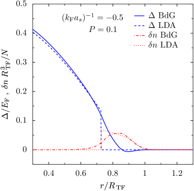
Figure 1: (color online) The gap $\Delta(r)$ and density difference $\delta n=n_{\uparrow}(r)$ – $n_{\downarrow}(r)$ profiles for the LDA and BdG calculations.

The existence of a PS for trapped, strongly interacting gases was indicated already in our earlier study Kinnunen et al. (2006), where the treatment of the trapping potential by Bogoliubov-de Gennes (BdG) equations revealed oscillations of the order parameter in an area located between the SF core and the N shell. Such oscillations resemble the nonuniform order parameter associated with the FFLO state, therefore we refer to these oscillations as "FFLO-type state". In this article, we show that the BdG analysis predicts such polarized superfluid in trapped Fermi gases not only as a shell effect but, for large polarizations, as a feature that extends through the whole system. We confirm that superfluidity and finite local density difference indeed co-exist in the center of the trap by calculating the condensate fraction, central gap and the core polarization. In previous works using BdG for trapped gases Castorina et al. (2005); Mizushima et al. (2005); Kinnunen et al. (2006); Machida et al. (2006) such an analysis, confirming the existence of a polarized superfluid in the center, was not performed. Moreover, the works Castorina et al. (2005); Mizushima et al. (2005); Machida et al. (2006) considered the weak interaction limit whereas we have extended the BdG calculation to the unitarity regime and actually consider the whole crossover from the BCS to BEC side. We analyze the dependence of the oscillations on the system size (particle number) and discuss the connection to phenomena occurring in superconductor - ferromagnet interfaces. For comparison, we also perform calculations using LDA. The LDA analysis predicts a polarized superfluid only at finite temperature, not at zero temperature like the BdG calculation. Therefore our results show that, in trapped Fermi gases, LDA has to be applied with care; beyond LDA approaches are not only needed for describing the interfaces of the system properly but, in some cases, features not predicted by LDA may become dominant.

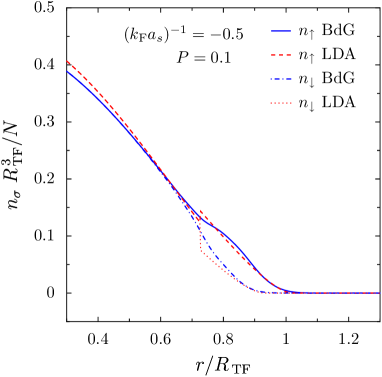
Figure 2: (color online) The density profiles of the $n_{\uparrow}(r)$ for BdG (solid) and LDA (dashed), and $n_{\downarrow}(r)$ for BdG (dot-dashed) and LDA (dotted).

This article is structured as follows. In section II. we present a review of the Bogoliubov - de Gennes (BdG) approach for describing pairing at the mean field level. We discuss the use of local density approximation, and the expansion in harmonic oscillator states as special cases of this general scheme. In the rest of the paper, we use the following terminology: BdG refers to the case where harmonic oscillator state basis has been used, and LDA to the use of local density approximation. The results are presented in section II. The appearance of the FFLO-type oscillations is discussed in subsection II.A and the case of large polarizations, when such oscillations span the whole system, is discussed in section II.B. We also analyze the dependence of these features on the interaction strength through the BCS-BEC crossover (section II.A.1.) and on the system size (atom number) (section II.A.2). The condensate fraction is calculated in section II.C. and the contributions of different harmonic oscillator states to the pairing are discussed in section II.D. Conclusions and discussion are presented in section III.

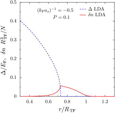
Figure 3: (color online) The gap and polarization profiles at slightly elevated temperature $T/T_{\mathrm{F}}=0.05$ for the LDA calculations and at low polarization. In contrast to the zero temperature case the thermal excitation in the BCS core starts to show up as a tail of the density difference into the core.

II Bogoliubov - de Gennes approach

In order to properly account for the inhomogeneity due to the presence of the trap potential we will in the following use the Bogoliubov-de Gennes equations de Gennes (1999), which in a more general context are also known as the selfconsistent Hartree-Fock-Bogoliubov equations. The imbalanced two-component Fermi gas is described by the grand canonical Hamiltonian

$$H = \sum_{\sigma}\int d^{3}\bm{r}\ \hat{\Psi}_{\sigma}^{\dagger}(\bm{r})\left(-\frac{\hbar^{2}\nabla^{2}}{2m}-\mu_{\sigma}+V(\bm{r})\right)\hat{\Psi}_{\sigma}(\bm{r})$$ (1)

$$+ \int d^{3}\bm{r}d^{3}\bm{r}^{\prime}\ \hat{\Psi}_{\uparrow}^{\dagger}(\bm{r})\hat{\Psi}_{\downarrow}^{\dagger}(\bm{r})U(\bm{r}-\bm{r}^{\prime})\hat{\Psi}_{\downarrow}(\bm{r})\hat{\Psi}_{\uparrow}(\bm{r}),$$

where $\hat{\Psi}_{\sigma}(\bm{r}),\hat{\Psi}_{\sigma}^{\dagger}(\bm{r})$ are the real space annihilation and creation operators for an atom with spin $\sigma$ at position $\bm{r}$, $\mu_{\sigma}$ is the chemical potential for the components $\sigma,$ $V(\bm{r})=\frac{1}{2}m\omega^{2}r^{2}$ is the external (isotropic and harmonic) trapping potential, and $U(\bm{r})=U\delta(\bm{r})$ is the interatomic atom-atom contact interaction potential. We apply the contact potential interaction and the mean-field approximation

$$U\hat{\Psi}_{\uparrow}^{\dagger}(\bm{r})\hat{\Psi}_{\downarrow}^{\dagger}(\bm{r})\hat{\Psi}_{\downarrow}(\bm{r})\hat{\Psi}_{\uparrow}(\bm{r}) \approx -\frac{\left|\Delta(r)\right|^{2}}{U}-Un_{\uparrow}(\bm{r})n_{\downarrow}(\bm{r})$$ (2)

$$+\,Un_{\uparrow}(\bm{r})\hat{\Psi}_{\downarrow}^{\dagger}(\bm{r})\hat{\Psi}_{\downarrow}(\bm{r})+Un_{\downarrow}(\bm{r})\hat{\Psi}_{\uparrow}^{\dagger}(\bm{r})\hat{\Psi}_{\uparrow}(\bm{r})$$

$$+\,\Delta(\bm{r})\hat{\Psi}_{\uparrow}^{\dagger}(\bm{r})\hat{\Psi}_{\downarrow}^{\dagger}(\bm{r})+\Delta^{\ast}(\bm{r})\hat{\Psi}_{\downarrow}(\bm{r})\hat{\Psi}_{\uparrow}(\bm{r}),$$

where $\Delta(\bm{r})=\langle\hat{\Psi}_{\downarrow}(\bm{r})\hat{\Psi}_{\uparrow}(\bm{r})\rangle$ and $n_{\sigma}(\bm{r})=\langle\hat{\Psi}_{\sigma}^{\dagger}(\bm{r})\hat{\Psi}_{\sigma}(\bm{r})\rangle$. The first two terms are simply numbers, so they are neglected. This gives the following mean-field Hamiltonian

$$H_{\mathrm{MF}} = \sum_{\sigma}\int d^{3}\bm{r}\ \hat{\Psi}_{\sigma}^{\dagger}(\bm{r})\left(-\frac{\hbar^{2}\nabla^{2}}{2m}-\mu_{\sigma}+V(\bm{r})\right)\hat{\Psi}_{\sigma}(\bm{r})$$ (3)

$$+ \sum_{\sigma}\int d^{3}\bm{r}\ Un_{\sigma}(\bm{r})\hat{\Psi}_{\bar{\sigma}}^{\dagger}(\bm{r})\hat{\Psi}_{\bar{\sigma}}(\bm{r})$$

$$+ \int d^{3}\bm{r}\left(\Delta(\bm{r})\hat{\Psi}_{\uparrow}^{\dagger}(\bm{r})\hat{\Psi}_{\downarrow}^{\dagger}(\bm{r})+\ \mathrm{H.c.}\right),$$

with $\bar{\sigma}$ being the other component of $\sigma.$ The second line is the mean-field Hartree corrections which represents an asymmetric shift to the chemical potential $\mu_{\sigma}$ of the gas of $\sigma$ atoms which is proportional to the density of the other component $n_{\bar{\sigma}}.$ In the Bogoliubov-de Gennes approach one expands the field operators on an appropriate basis set, dictated by the symmetries of the non-interacting part of the Hamiltonian and usually characterized by a set $\{\eta\}$ of good quantum numbers, in order to diagonalize the Hamiltonian as in the uniform case. In the balanced non-uniform case and in the absence of superflow the generalized BCS pairing is in general between atoms in time-reversed states. The problem can now be solved by introducing the generalized canonical Bogoliubov-Valatin transformation to the new fermionic operators $\alpha_{\eta},\alpha_{\eta}^{\dagger}$ which amounts to the expansion

$$\hat{\Psi}_{\sigma}(\bm{r})=\sum_{\eta}u_{\eta}(\bm{r})\hat{\alpha}_{\eta\sigma}-s_{\sigma}v_{\eta}^{\ast}(\bm{r})\hat{\alpha}_{\bar{\eta}\bar{\sigma}}^{\dagger},$$

where the overhead bar designates the quantum numbers of the time-reversed state for $\eta$ and the other hyperfine spin state for $\sigma,$ and with $s_{\uparrow}=1,s_{\downarrow}=-1.$ We note that in the analogous case of electronic pairing in superconductors $\bar{\sigma}$ denote the time-reversed spin part of the wavefunction. From the requirement that the new operators $\alpha_{\eta},\alpha_{\eta}^{\dagger}$ diagonalize the Hamiltonian (3) one derives the matrix Bogoliubov-de Gennes equation de Gennes (1999)

$$(\hat{H}_{0}\hat{\tau}_{3}-\hat{\Delta}\hat{\tau}_{1})\bm{\varphi}_{\eta}=E_{\eta}\bm{\varphi}_{\eta}(\bm{r}),$$ (4)

for the spinor $\bm{\varphi}(\bm{r})\equiv(u_{\eta}(\bm{r}),v_{\eta}(\bm{r}))$, where $\eta$ denotes a set of appropriate quantum numbers and $u_{\eta},v_{\eta}$ are therefore to be regarded as subspinors, $\hat{H}_{0}$ is the non-interacting diagonal part of the Hamiltonian, potentially including a trapping potential and Hartree shifts to the chemical potentials, $\hat{\Delta}$ is the pairing field part of the Hamiltonian, $E_{\eta}$ is the eigenenergy. The products with the Pauli matrices $\hat{\tau}_{i}$ on the left hand side of Eq. (4) are to be understood as a direct products. The selfconsistent aspect of the method is due to the fact that the chemical potentials, mean-field Hartree and pairing fields are to be selfconsistently determined through the gap and number equations. The details of the BdG calculation for the harmonic trap eigenstates are presented in Section II.2. Next we turn to the discussion of the local density approximation.

II.1 Local density approximation

We first consider the local density approximation which is assumed to be valid for sufficiently large condensates. The starting point for the LDA calculation is to solve the problem in the uniform case. The translational invariance of a uniform superfluid implies that the plane wave states $\hat{\Psi}(\bm{r)}=\mathcal{V}^{-1/2}\sum_{\bm{k}}e^{i\bm{k}\cdot\bm{r}}a_{\bm{k}}$ can be used to diagonalize the Hamiltonian. The main assumption of the LDA is that the system is locally homogeneous and therefore we initially consider the Hamiltonian $H$ in (5) for a uniform system (i.e. $V(r)=0$) with contact interactions, which in the momentum representation reads

$$H=\sum_{\bm{k},\sigma}\varepsilon_{\bm{k}}a_{\bm{k}\sigma}^{\dagger}a_{\bm{k}\sigma}+\frac{U}{\mathcal{V}}\sum_{\bm{k},\bm{k}^{\prime}}a_{\bm{k}\uparrow}^{\dagger}a_{\bm{k}\downarrow}^{\dagger}a_{-\bm{k}^{\prime}\downarrow}a_{\bm{k}^{\prime}\uparrow},$$ (5)

where $a_{\bm{k}\sigma}^{\dagger},a_{\bm{k}\sigma}$ are the creation and annihilation operators for free atoms with momentum $\hbar\bm{k}$, and the kinetic energy $\varepsilon_{\bm{k}}=\hbar^{2}k^{2}/(2m)$. The chemical potentials $\mu_{\sigma}$ are introduced as Lagrange multipliers for the particle numbers $N_{\sigma}$. We define the average chemical potential $\mu=(\mu_{\uparrow}+\mu_{\downarrow})/2$ and the imbalance potential $\delta\mu=(\mu_{\uparrow}-\mu_{\downarrow})/2$, such that $\mu_{\sigma}=\mu+s_{\sigma}\delta\mu,$ with $s_{\sigma}$ defined as above. Within the mean field approximation the Hamiltonian can be diagonalized by the standard Bogoliubov-Valatin transformation. In the uniform case the order parameter is the usual $\Delta=\langle a_{\bm{k}\uparrow}a_{-\bm{k}\downarrow}\rangle$ which satisfies the gap equation. Within the semiclassical approximation the gap $\Delta(r)$ is assumed to depend weakly on the radial position $r=|\bm{r}|$ and, as is commonly done, we introduce the local chemical potential $\mu_{\sigma}\to\mu_{\sigma}(r)=\mu_{\sigma}-V(r),$ where $V(r)$ is the trapping potential. The quasi-particle dispersions depend on the gap and therefore on the radial position through the local chemical potentials and the gap profile. In the most general case the quasi-particle dispersion relation becomes

$$E_{\bm{k}\sigma}(\bm{r})=\frac{1}{2}\left(\xi_{\bm{k}\sigma}(r)-\xi_{\bm{k}\bar{\sigma}}(r)\right)+E_{\bm{k}}(r),$$

where $E_{\bm{k}}(r)=[\xi_{\bm{k}}(r)+\Delta^{2}(r)]^{1/2},$ with $\xi_{\bm{k}}(r)=\left(\xi_{\bm{k}\sigma}(r)+\xi_{\bm{k}\bar{\sigma}}(r)\right)/2,$ and $\xi_{\bm{k}\sigma}(r)=\hbar^{2}k^{2}/(2m)-\mu_{\sigma}(r).$ As we will assume pairing between atoms with equal mass we get $E_{\bm{k}\sigma}=-s_{\sigma}\delta\mu+E_{\bm{k}},$ and therefore ${2E}_{\bm{k}}=E_{\bm{k}\sigma}+E_{\bm{k}\bar{\sigma}},$ and $\xi_{\bm{k}}=\varepsilon_{\bm{k}}-\mu(r)$ with $\mu,\delta\mu$ defined above. Within LDA, both the gap and the local chemical potentials depend on the radial position and therefore the system may in general be locally polarized. We define an averaged Fermi energy scale $E_{\mathrm{F}}$ from the total atom number $N=[E_{\mathrm{F}}/(\hbar\omega)]^{3}/3$, for a balanced non-interacting Fermi gas in a harmonic trap potential $V(r)=m\omega^{2}r^{2}/2$, where $\omega$ is the trap frequency. The characteristic scale of the size of the cloud is the Thomas-Fermi radius is $R_{\mathrm{TF}}=[2E_{\mathrm{F}}/(m\omega^{2})]^{1/2}$. Within LDA the local gap equation at position $f$ reads

$$1=\frac{U_{\ast}}{\mathcal{V}}\sum_{\bm{k}}\left[\frac{1}{2\varepsilon_{\bm{k}}}-\frac{1-n_{\mathrm{F}}(E_{\bm{k}\uparrow}(r))-n_{\mathrm{F}}(E_{\bm{k}\downarrow}(r))}{2E_{\bm{k}}(r)}\right],$$ (6)

with $U_{\ast}=4\pi\hbar^{2}a_{s}/m$ being the usual regularized effective interaction strength which replaces the bare interaction $U,$ and $a_{s}$ is the $s$-wave scattering length, and where we have regularized the ultraviolet divergence appearing momentum integrals arising from unphysical properties of the contact interaction Fetter and Walecka (1971). The gap equation is an implicit equation for the gap profile $\Delta(\bm{r})$ Perali et al. (2003) which for an isotropic trap is only a function of the radial position $r=|\bm{r}|$. The number equation and the density profiles are determined from the thermodynamic relation

$$N_{\sigma} = -\frac{\partial\Omega}{\partial\mu_{\sigma}}=\int d^{3}\bm{r}\ n_{\sigma}(r),$$

where the radial distribution for the $\sigma$ component is

$$n_{\sigma}(r)=\frac{1}{\mathcal{V}}\sum_{\bm{k}}\left[u_{\bm{k}}^{2}n_{\mathrm{F}}(E_{\bm{k}\sigma}(r))+v_{\bm{k}}^{2}n_{\mathrm{F}}(-E_{\bm{k}\bar{\sigma}}(r))\right],$$

with $\bar{\sigma}$ denotes the other component of $\sigma.$ The polarization $P$ is

$$P=\frac{N_{\uparrow}-N_{\downarrow}}{N_{\uparrow}+N_{\downarrow}}=\frac{1}{N}\int d^{3}r\ \delta n(r),$$ (7)

where $\delta n(r)=n_{\uparrow}(r)-n_{\downarrow}(r).$ The equations for the polarization $P$ and for the minority component $N_{\downarrow}/N=(1-P)/2$ are numerically solved by iteration together with the gap profile as follows. We first make an initial guess for the values of the chemical potentials $\mu$ and $\delta\mu$ at fixed coupling $k_{\mathrm{F}}a_{s}.$ The $r$ dependent gap $\Delta(r)$, minor density $n_{\downarrow}(r)$ and polarization density $\delta n(r)$ are then discretized on a radial grid of sufficient resolution. From the initial values of $\mu$ and $\delta\mu$ and at fixed coupling the gap profile $\Delta(r)$ is calculated by solving the gap equation (6) as a root problem. The gap profile is then subsequently used to calculate the densities $n_{\downarrow}(r)$ and $\delta n(r)$ as functions of $\mu$ and $\delta\mu.$ The minor number and and polarization equations are then solved as a multidimensional root problem for the average chemical potential $\mu$ and the bare depairing width $\delta\mu.$ The system of equations are iterated until the gap profile and the chemical potentials are sufficiently converged and then finally $n_{\uparrow}(r)=\delta n(r)+n_{\downarrow}(r).$ The present method applied here is well suited for considering effects of the Hartree terms, but we have not included those in the results presented here.

II.2 Harmonic trap eigenstates

The Bogoliubov-de Gennes (BdG) approach allows treating the effect of the harmonic trapping potential exactly. The approach has been used for polarized Fermi gases Castorina et al. (2005); Mizushima et al. (2005); Kinnunen et al. (2006); Machida et al. (2006) because it avoids some of the problems of a local density approximation approach. We have used it in our previous work Kinnunen et al. (2006) and give in this section a detailed description of the calculations on which the results in Kinnunen et al. (2006) and in this article are based. One particularly important advantage of this approach is the proper description of interface effects in a phase separated gas, following from the nonlocal nature of the solution and the wavefunctions. Eventually, in the limit of a large number of atoms, the LDA and BdG solutions are expected to become the same.

The BdG approach used here is a generalization, to the imbalanced densities case, of the calculation outlined in Ref. Ohashi and Griffin (2005) which was for an unpolarized Fermi gas. For the imbalanced case the generalization amounts to introducing different chemical potentials $\mu_{\downarrow}$ and $\mu_{\uparrow}$ for the two species of fermionic atoms. We now expand the wavefunctions $\hat{\Psi}_{\sigma}(\bm{r})$ in the basis of the 3D harmonic oscillator eigenstates

$$\hat{\Psi}_{\sigma}(\bm{r})=\sum_{nlm}R_{nl}(r)Y_{lm}(\hat{r})\hat{a}_{nlm\sigma},$$ (8)

where the quantum numbers $\{\eta\}\equiv\{n,l,m\}$ are the radial quantum number $n$ counting the nodes in the radial function, $l$ is the orbital angular momentum and $m$ is the projected angular momentum onto the axis of quantization. Here $Y_{lm}(\hat{r})$ are the spherical harmonics with $\hat{r}=(\theta,\varphi)$ and the radial part of the wavefunction is

$$R_{nl}(r)=\sqrt{2}\left(m\omega\right)^{3/4}\sqrt{\frac{n!}{\left(n+l+1/2\right)!}}e^{-\bar{r}^{2}/2}\bar{r}^{l}L_{n}^{l+1/2}\left(\bar{r}^{l}\right),$$ (9)

where $\bar{r}=r/a_{\mathrm{osc}}$ with the harmonic oscillator length being $a_{\mathrm{osc}}=[\hbar/(m\omega)]^{1/2},$ and $L_{n}^{l+1/2}(\bar{r}^{2})$ is an associated Laguerre polynomial. The characteristic scale of the cloud is given by the Thomas-Fermi radius $R_{\mathrm{TF}}^{2}=2E_{\mathrm{F}}/(m\omega^{2})$ and therefore $R_{\mathrm{TF}}=(24N)^{1/6}a_{\mathrm{osc}}$. The spherical symmetry allows doing the angular integrations, and getting rid of the $m$-quantum numbers, thereby making the $l$-states $(2l+1)$-fold degenerate. The expansion yields the following Hamiltonian

$$H_{\mathrm{MF}} = \sum_{n,l,\sigma}(2l+1)\left(\varepsilon_{nl}-\mu_{\sigma}\right)a_{nl\sigma}^{\dagger}a_{nl\sigma}$$ (10)

$$+ U\sum_{n,n^{\prime},l,\sigma}J_{nn^{\prime}\bar{\sigma}}^{l}a_{nl\sigma}^{\dagger}a_{n^{\prime}l\sigma}$$

$$+ \sum_{n,n^{\prime},l}F_{nn^{\prime}}^{l}a_{nl\uparrow}^{\dagger}a_{n^{\prime}l\downarrow}^{\dagger}+\mathrm{H.c}.$$

Here the single particle energies are $\varepsilon_{nl}=\hbar\omega\left(2n+l+3/2\right)$, and the Hartree interaction is described by the elements

$$J_{nn^{\prime}\sigma}^{l}=\int_{0}^{\infty}dr\ r^{2}R_{nl}(r)n_{\sigma}(r)R_{n^{\prime}l}(r),$$

and the pairing field is described by

$$F_{nn^{\prime}}^{l}=\int_{0}^{\infty}dr\ r^{2}R_{nl}(r)\Delta(r)R_{n^{\prime}l}(r).$$

We note that the $\sigma$ dependence of the Hartree term is due to the population imbalance which implies that the corrections are different for the two components. The density of $\sigma$ atoms is

$$n_{\sigma}(r)=\sum_{n,n^{\prime},l}\frac{2l+1}{4\pi}R_{nl}(r)R_{n^{\prime}l}(r)\langle a_{nl\sigma}^{\dagger}a_{n^{\prime}l\sigma}\rangle,$$ (11)

and the order parameter is

$$\Delta(r)=\tilde{U}(r)\sum_{n,n^{\prime},l}\frac{2l+1}{4\pi}R_{nl}(r)R_{n^{\prime}l}(r)\langle a_{nl\uparrow}^{\dagger}a_{n^{\prime}l\downarrow}^{\dagger}\rangle.$$ (12)

The additional factor $(2l+1)$ comes from the degeneracy of the $l$-states, obtained by the summation over the $m$ states. The renormalized interaction strength $\tilde{U}(r)$ will be described later.

Truncating the Hilbert space by keeping only the states with single-particle energies $\varepsilon_{nl}\leq E_{\mathrm{c}}$ allows writing the Hamiltonian in a matrix form that can be diagonalized. Noticing that the Hamiltonian commutes for different $(l)$-quantum numbers makes it possible to diagonalize each $(l)$-matrix separately, simplifying the problem significantly. For a given $(l)$-quantum numbers the Hamiltonian reads

$$H_{\mathrm{MF}}^{(l)}=\left(\begin{array}[]{c}a_{0l\uparrow}^{\dagger}\\ \ldots\\ a_{N_{l}l\uparrow}^{\dagger}\\ a_{0l\downarrow}\\ \ldots\\ a_{N_{l}l\downarrow}\end{array}\right)^{T}M^{l}\left(\begin{array}[]{c}a_{0l\uparrow}\\ \ldots\\ a_{N_{l}l\uparrow}\\ a_{0l\downarrow}^{\dagger}\\ \ldots\\ a_{N_{l}l\downarrow}^{\dagger}\end{array}\right),$$ (13)

where $N_{l}=[E/(\hbar\omega)-l-3/2]/2$ is the $l$-specific cutoff (yielding the correct energy cutoff) and $M^{l}$ is a $2(N_{l}+1)\times 2(N_{l}+1)$-dimensional orthogonal matrix. Notice that the $\downarrow$ states have been turned into holes by switching the order of $a_{\downarrow}^{\dagger}$ and $a_{\downarrow}$ operators as suggested by the ordinary Bogoliubov transformation. The matrix $M^{l}$ is now

$$M^{l}=\left(\begin{array}[]{cccccc}\varepsilon_{0l}-\mu_{\uparrow}+UJ_{00\downarrow}^{l}&\ldots&UJ_{{0N}_{l}\downarrow}^{l}&F_{00}^{l}&\ldots&F_{{0N}_{l}}^{l}\\ \ldots&\ldots&\ldots&\ldots&\ldots&\ldots\\ UJ_{N_{l}0\downarrow}^{l}&\ldots&\varepsilon_{N_{l}l}-\mu_{\uparrow}+UJ_{N_{l}N_{l}\downarrow}^{l}&F_{N_{l}0}^{l}&\ldots&F_{N_{l}N_{l}}^{l}\\ F_{00}^{l}&\ldots&F_{N_{l}0}^{l}&-\varepsilon_{0l}+\mu_{\downarrow}-UJ_{00\uparrow}^{l}&\ldots&-UJ_{N_{l}0\uparrow}^{l}\\ \ldots&\ldots&\ldots&\ldots&\ldots&\ldots\\ F_{0N_{l}}^{l}&\ldots&F_{N_{l}N_{l}}^{l}&-UJ_{0N_{l}\uparrow}^{l}&\ldots&-\varepsilon_{N_{l}l}+\mu_{\downarrow}-UJ_{N_{l}N_{l}\uparrow}^{l}\end{array}\right).$$ (14)

Diagonalizing this Hamiltonian corresponds to the Bogoliubov transformation, which yields the eigenenergies $E_{jl}$ and the corresponding quasiparticle eigenstates ($2(N_{l}+1)$-dimensional vectors) $W_{jn}^{l}$. The indices $j,n$ both run from $0$ to ${2N}_{l}+1.$ In the basis of these quasiparticle states, the Hamiltonian is

$$H_{MF}^{(l)}=\sum_{j=0}^{2N_{l}+1}E_{jl}\alpha_{jl}^{\dagger}\alpha_{jl}.$$ (15)

In this basis, the density of atoms in $\uparrow$ state is

$$n_{\uparrow}(r) = \sum_{l}\frac{2l+1}{4\pi}\sum_{j}\sum_{n,n^{\prime}=0}^{2N_{l}+1}R_{nl}(r)R_{n^{\prime}l}(r)$$ (16)

$$\times W_{jn}^{l}W_{jn^{\prime}}^{l}n_{\mathrm{F}}(E_{jl}),$$

where the Fermi distribution $n_{\mathrm{F}}(E)=1/(1+e^{E/k_{\mathrm{B}}T})$. Likewise, the density of atoms in $\downarrow$ state is

$$\begin{split}n_{\downarrow}(r)=\sum_{l}\frac{2l+1}{4\pi}&\sum_{j}\sum_{n,n^{\prime}=0}^{2N_{l}+1}R_{nl}(r)R_{n^{\prime}l}(r)\\ &\times W_{j,n+N_{l}+1}^{l}W_{j,n^{\prime}+N_{l}+1}^{l}n_{\mathrm{F}}(-E_{jl}),\end{split}$$ (17)

where the sign in the Fermi function is changed because of the $\downarrow$ component (the last $N_{l}+1$ components) of the eigenstates correspond to holes as compared to the particles in the $\uparrow$ components (the first $N_{l}+1$ components). The order parameter is given by

$$\Delta(r) = \sum_{l}\frac{2l+1}{4\pi}\sum_{j}\sum_{n,n^{\prime}=0}^{{2N}_{l}+1}R_{nl}(r)R_{n^{\prime}l}(r)$$ (18)

$$\times W_{jn}^{l}W_{j{,n}^{\prime}+N_{l}+1}^{l}\left(1+2n_{\mathrm{F}}(E_{jl})\right).$$

The total number of atoms in the two components can be obtained by integrating over the densities. However, numerically it is faster to calculate them directly from the eigenstates using the equations

$$N_{\uparrow}=\sum_{l}(2l+1)\sum_{j}\sum_{n=0}^{2N_{l}+1}W_{jn}^{l}W_{jn}^{l}n_{\mathrm{F}}(E_{jl})$$ (19)

and

$$N_{\downarrow}=\sum_{l}(2l+1)\sum_{j}\sum_{n=0}^{2N_{l}+1}W_{j,n+N_{l}+1}^{l}W_{j,n+N_{l}+1}^{l}n_{\mathrm{F}}(-E_{jl}).$$ (20)

The gap and the number equations (18,19,20) are solved iteratively. We have made calculations where the Hartree fields are included and compared them to the case where Hartree fields are neglected by setting $J_{nn^{\prime}\sigma}^{l}=0$ for all $n,n^{\prime},l$ . Note that close to the Feshbach resonance, the Hartree fields become formally infinite. In this extreme limit, we have limited the Hartree interaction strength $U$ to $\left|\left(k_{\mathrm{F}}a_{s}\right)^{-1}\right|\leq\beta$, where $\beta\approx 0.5$. When comparing the results with and without Hartree fields, there is no difference in the qualitative features such as the order parameter oscillations and over-all shape of the gap and density profiles, the Hartree fields cause only minor corrections to gap and density profiles (effectively compressing the gas slightly). Numerically, neglecting the Hartree fields gives a tremendous speedup in the numerical solution because it decouples the density and gap profiles. In the results presented in this article, the Hartree fields are neglected. We have made the calculations at zero temperature and present here only results at $T=0$. We have checked that the BdG results do not change by using a finite but very small temperature $T=0.001\ T_{\mathrm{F}}$.

As the density and gap profiles are decoupled, it is straightforward to solve the gap equation for given chemical potentials. However, since we want to keep the number of atoms fixed, the total procedure will require optimizing also the chemical potentials, so that the number equations are satisfied. The subsequent iteration procedure can be performed in several different ways. We have found that a very efficient procedure is to solve the chemical potentials (by solving the number equations (19,20)) for each trial gap profile $\Delta(r)$. The trial gap profile $\Delta(r)$ is then used for solving the new trial gap profile $\Delta^{\prime}(r)$ using the gap equation (18) with the new obtained chemical potential. The chemical potentials therefore keep changing between the iteration steps of the gap profile. On the other hand, the numbers of atoms stay fixed in the iteration process.

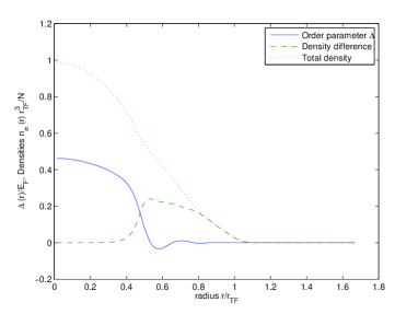
Figure 4: (color online) Gap and density profiles on the BCS side of the resonance $(k_{\mathrm{F}}a_{s})^{-1}=-0.5$ for $P=0.50.$

The initial guesses for the profiles needed for the iteration procedure are obtained by using the chemical potentials and the gap profile obtained for a slightly lower polarization and, eventually, by the solution obtained for unpolarized gas. Solution of the profiles for a given polarization $P$ requires therefore solving the profiles for all lower polarizations. The validity of the final solution $\Delta(r),\mu_{\uparrow},\mu_{\downarrow}$ has been checked for several values of polarization and interaction strength by perturbing the final solution and using the perturbed profiles $\Delta^{\prime}(r),\mu_{\uparrow},\mu_{\downarrow}$ as initial guesses for the profiles. Usually the disturbed profiles have converged either into the final profiles $\Delta(r)$ or into the normal state $\Delta(r)\equiv 0$. Only in the regime where our calculations predict the superfluid core polarization have our solutions sometimes strayed into a superfluid solution with unpolarized core. In such cases, the final solution has been picked by choosing the solution with the lower total energy, given by

$$\begin{split}E=\sum_{l}^{2N_{l}+1}(2l+1)&\left[\sum_{n}\left(\varepsilon_{nl}-\mu_{\downarrow}\right)+\sum_{j}E_{jl}n_{\mathrm{F}}(E_{jl})\right]\\ &-\frac{1}{\tilde{U}(r)}\int dr\ r^{2}|\Delta(r)|^{2},\end{split}$$ (21)

where the first (constant) term comes from switching to use the hole states in the $\downarrow$ component (and this is countered by having half of the eigenenergies $E_{jl}$ negative). The last term follows from the mean-field term $\langle\hat{\Psi}_{\uparrow}^{\dagger}(\bm{r})\hat{\Psi}_{\downarrow}^{\dagger}(\bm{r})\rangle\langle\hat{\Psi}_{\downarrow}(\bm{r})\hat{\Psi}_{\uparrow}(\bm{r})\rangle$ which was dropped from the mean-field Hamiltonian because it is a number, not operator.

The summation in the gap equation (18) is divergent without the energy cutoff $E_{\mathrm{c}}.$ This is a well known phenomenon, following from the incapability of the contact interaction potential to describe properly high energy behavior. Several different regularization schemes have been proposed Bruun et al. (1999); Bulgac and Yu (2002); Grasso and Urban (2003), and here we apply the one suggested in Ref. Grasso and Urban (2003). This implies the following form for the renormalized coupling

$$\frac{1}{\tilde{U}(r)}=\frac{1}{U}+\frac{1}{2\pi^{2}}\left(\frac{k_{\mathrm{F}}^{0}(r)}{2}\ln\left(\frac{k_{c}(r)+k_{\mathrm{F}}^{0}(0)}{k_{c}(r)-k_{\mathrm{F}}^{0}(0)}\right)-k_{c}(r)\right),$$

where the momentum cutoff $k_{c}(r)=(2N_{c}+3-r^{2})^{1/2}$ and the local Fermi momentum $k_{\mathrm{F}}^{0}(r)=(\mu_{\uparrow}+\mu_{\downarrow}-r^{2})^{1/2}$ for the imbalanced case compared to Eq. (14) and Eq. (18) of Ref. Grasso and Urban (2003), respectively. On the BCS side of the resonance for $\left(k_{\mathrm{F}}a_{s}\right)^{-1}<0$ we have used as the cutoff $E_{\mathrm{c}}=200\ \hbar\omega$ and on the BEC side for $\left(k_{\mathrm{F}}a_{s}\right)^{-1}>0$ the cutoff $E_{\mathrm{c}}=240\ \hbar\omega$ was used. We have tested the remaining cutoff dependence by using the cutoff $300\ \hbar\omega.$ Depending on the number of atoms, the cutoff dependence in the gap profiles was at most $2\%.$

III Results

The results show two features that we will discuss in detail below: 1) For small and intermediate polarizations, FFLO-type oscillations in the superfluid-normal interface at the edge of the trap, 2) for large polarization, a polarized superfluid that extends through the whole trapped gas. We study the behavior of these features, especially 1), throughout the BCS-BEC crossover and when the system size, i.e. the atom number, is varied. We also calculate the condensate fraction to make a connection to experiments. Finally, we analyze which harmonic oscillator states are involved in pairing for different polarizations and discuss the connection and differences to FFLO-state in a homogeneous space.

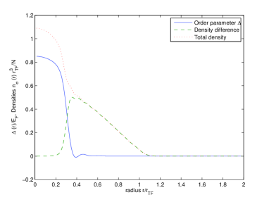
Figure 5: (color online) Typical profiles at resonance $(k_{\mathrm{F}}a_{s})^{-1}=0.0$ for $P=0.9.$

III.1 FFLO-type oscillations

Typical density and gap profiles at $T=0$, for small polarization, are shown in Figs. 1 and 2, both for LDA and BdG. Comparison of the profiles gives the following general picture: BdG predicts a) SF (equal densities) core, b) PS (FFLO-like oscillations) shell, c) normal state shell of the majority component $N_{\uparrow}.$ LDA predicts a) SF (equal densities) core, b) normal state shell; the absence of the PS shell in LDA is reflected in the discontinuity of the density and gap profiles at the SF-N phase boundary. At finite temperatures, also LDA shows a polarized shell and the boundary becomes continuous, only showing a kink (Fig. 3). As shown by Figs. 1-3, for small polarization the PS given by BdG calculations is a narrow shell and can be understood as a boundary effect. However, in the following we show that, for large polarization, the FFLO-features extend to the center of the trap as well.

A seen from Fig. 1 and Fig. 3 the general results from LDA and BdG calculation agree fairly well and the overall agreement for the gap and density profiles becomes better for increasing particle number. The incapability of LDA to correctly describe the short scale behavior (explicitly excluded by LDA) leads to the unphysical appearance of a discontinous order parameter solution and can be viewed as a breakdown of LDA near the interface much in the same way as LDA generally breaks near the edge of a balanced condensate. The breakdown of LDA is however more pronounced in the imbalanced case due to presence of the normal shell surrounding the condensate which leads to separation of the size of the condensate and the size of the cloud.

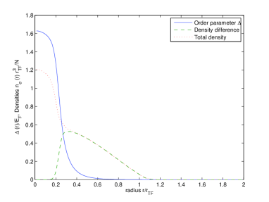
Figure 6: (color online) Gap and density profiles on the BEC side of the resonance $(k_{\mathrm{F}}a_{s})^{-1}=0.5$ for P=0.95.

III.1.1 Dependence on the interaction strength – BCS-BEC crossover

We present here results for three different cases: (1) BCS side of the crossover, $(k_{\mathrm{F}}a_{s})^{-1}=-0.50$, (2) unitarity, that is, $(k_{\mathrm{F}}a_{s})^{-1}=0$, (3) BEC side $(k_{\mathrm{F}}a_{s})^{-1}=0.50$. We focus on the behavior at strong interactions since the cases (1)-(3) can all be considered to be at the unitarity regime (if it is defined $|(k_{\mathrm{F}}a_{s})^{-1}|<1$ ) although representing different sides of the crossover. We do not consider the extreme BCS limit of weak interactions because the features and trends observed in the unitarity limit are also expected to appear at weaker coupling.

For attractive interactions, $(k_{\mathrm{F}}a)^{-1}<0$, the typical density and order parameter profiles looks as shown in Fig. 4 for polarization $P=0.50$. In agreement with earlier studies using the same approach Castorina et al. (2005); Mizushima et al. (2005); Kinnunen et al. (2006); Machida et al. (2006), the solution reveals an unpolarized BCS-type region at the center of the trap and a polarized shell with oscillating order parameter. The oscillations rapidly dampen when the density of the minority component drops.

We have studied the presence of the oscillations around the unitarity region, and noticed that the critical polarization for the appearance of the order parameter oscillations increases with stronger interactions. At unitarity ($(k_{\mathrm{F}}a)^{-1}=0.0$), the order parameter oscillations did not appear until polarization $P=0.70$, compared to $P=0.10$ at $(k_{\mathrm{F}}a)^{-1}=-0.50$. The disappearance of the oscillations follows from the enhanced stability of the BCS-type pairing at stronger interactions, making the increased distortion of the minority component density profile favorable over the reduced order parameter due to the polarization. The result at unitarity is shown in Fig. 5.

On the BEC side, the oscillations do not appear. We have made calculations for several parameters on the BEC side of the resonance and have not found any FFLO-type oscillations in the order parameter on the BEC side. This is consistent with the observation discussed above that the critical polarization for the emergence of the nodes in the order parameter increases with increasing interaction strength. The same qualitative results on the BCS-BEC crossover were recently obtained in Mizushima et al. (2007) using a hybrid BdG-LDA scheme in a cylindrically symmetric geometry. Typical density and gap profiles on the BEC side are shown in Fig. 6.

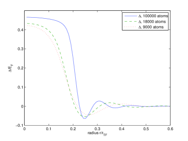
Figure 7: (color online) Gap profiles at $(k_{\mathrm{F}}a_{s})^{-1}=-0.5$ for several values $N=9000,18000,100000$ of the total number of particles at a high and fixed polarization $P=0.74.$ For increasing particle number the transition from an almost constant value of the gap in the BCS core to the oscillating gap at the edge becomes sharper. For increasing particle number the gap FFLO-like oscillations at the edge the cloud display shorter wavelength and a slight increase in amplitude.

III.1.2 Dependence on the system size - atom number N

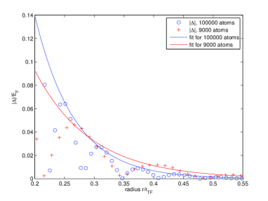
Figure 8: (color online) Exponential fits for the envelopes of the order parameter oscillations for 9000 and 100000 atoms.

We have studied the dependence of the results on the number of atoms by performing the BdG calculations for the total atom numbers 9000, 10000, 18000, 20000 and 100000. Note that this means substantial increase in the system size compared to our earlier work Kinnunen et al. (2006) where the atom number 10000 was used.

The order parameter oscillations for different numbers of atoms are shown in Fig. 7. In Fermi units (i.e. in the cloud scale $R_{\mathrm{TF}}$), the wavelength of the oscillations becomes shorter with the increased atom number but, on the other hand, more nodes appear. The scaling of all these factors is complicated, but insight can be obtained by fitting an exponential function $\sim e^{-x/\xi}$ to the envelope of the order parameter oscillations as shown in Fig. 8. The exponential decay gives a very good description for the damping of the oscillations with increasing distance from the trap center $r$. The penetration depths $\xi$ obtained from the fitting indeed slowly decrease in Fermi units when the atom number $N$ is increased, the scaling being roughly $N^{1/6}$. Since $R_{\mathrm{TF}}\propto N^{1/6}$, one may anticipate that the decrease of the penetration depth only occurs in relative scale, not absolute. Indeed, in a microscopic length scale (harmonic oscillator units $a_{\mathrm{osc}}$) the penetration depth remains constant, being $0.54\ a_{\mathrm{osc}}$ for 100000 atoms and $0.56\ a_{\mathrm{osc}}$ for 9000 atoms. These observations confirm that the order parameter oscillations are not a finite size effect but rather an interface effect for the superfluid-normal interface. From the shape of the order parameter profile it can be seen that that the interface formed becomes sharper for increasing particle number and we therefore suggest that the interface forming at the edge is an analog of the proximity effects appearing in superfluid-normal and superfluid-ferromagnetic junctions. In the latter case it has been shown that the interplay between BCS superconductivity and ferromagnetic order (in our case the polarization $\delta n$) gives rise to an oscillating order parameter which decays anomalously slow (over several oscillations) on the ferromagnet side and with a characteristic length scale that is independent of the properties of the superconductor Demler et al. (1997); Kontos et al. (2001); Schaeybroeck and Lazarides (2007). An interesting question is the dependence of the penetration depth on the interaction strength and polarization. However, we have not been able to pursue this question in more detail here and leave it for future work.

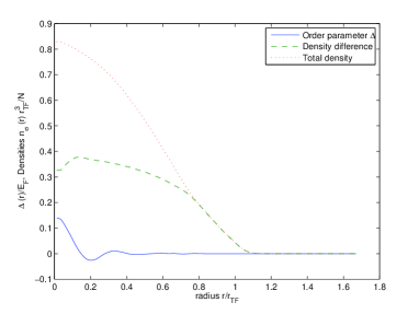
Figure 9: Density and order parameter profiles at $P=0.762$ and $(k_{\mathrm{F}}a_{s})^{-1}=-0.50$ for $N=9000$ show the superfluid with core polarization, together with a small dip in the density difference at the center of the trap.

In this context, we believe a few remarks on the work Liu et al. (2007) are in order. It is argued in Liu et al. (2007), based on a hybrid BdG-LDA scheme (no analysis of the penetration depths as presented above was done in Liu et al. (2007)), that the oscillations of the order parameter vanish for sufficiently large particle number and are thus interpreted as a finite size effect. It is argued that as the cutoff energy $E_{c}$ introduced to separate the BdG and the LDA scales in the hybrid scheme goes to zero, LDA should be recovered. This is of course self-evident due to the construction of the hybrid algorithm but reducing the cutoff energy without concern may lead to missing some features of the system. The fact that a sharp interface with increasingly microscopic features (oscillations with short period on the scale of the cloud size) builds up for increasing number of particles requires $E_{c}$ to be increased significantly in order to resolve the short length scale features. Consistent with our results, Fig. 4 in Liu et al. (2007) shows that the order parameter oscillates with a shorter period, and at the same time the amplitude of the order parameter slowly increases, for increasing particle number. The recent results for a hybrid BdG-LDA scheme Mizushima et al. (2007) and the scaling analysis therein agree well with the results given by our full BdG calculations.

III.2 Polarized superfluid for large imbalances

When the polarization $P$ exceeds some (large) critical value, the FFLO-type oscillations discussed above reach the center of the trap. At this point the gas becomes polarized also at the center of the trap and the order parameter drops to roughly half of its unpolarized BCS value. This realizes a superfluid with finite polarization throughout the system. Fig. 9 shows the density and order parameter profiles for $P=0.762$. For such a core polarized system, the concept of an interface effect is intriguing as there is no BCS-type superfluid core present.

The density difference for such a polarized superfluid shows an interesting feature: a small dip in the center of the trap (i.e. the density difference is smaller than in the surrounding area, but still non-zero). At zero temperature, this feature only appears in our BdG calculations whereas LDA, which fails to predict a polarized superfluid at $T=0$, does not lead to such a dip in the density difference. In contrast, LDA calculations at finite temperature produce such a feature in connection with the finite temperature BP phase. Recent Monte Carlo studies of the trapped Fermi gas have shown that, for the strongly interacting normal state, the density difference increases monotonously towards the center of the trap Lobo et al. (2006). Therefore one may argue that the dip is associated with a polarized superfluid: at $T=0$ it is FFLO-type, at temperatures that are finite but clearly below the critical temperature it is either FFLO or BP. At higher temperatures, pseudogap effects may contribute to such features as well Chien et al. (2006). Such a dip can be seen in the experimental results of Shin et al. (2006).

The interaction strength dependence of such a polarized superfluid with oscillating order parameter is similar to what was already discussed above. Since there are no order parameter oscillations on the BEC side, we have also not seen any core polarized superfluid either. Of course, there does exist a different kind of core polarization on the BEC side: coexistence of a molecular condensate and free excess fermions, but that is not associated with oscillating order parameter.

The parameter window for the polarized superfluid shrinks with increasing atom number $N$. For $9000$ atoms the window is $0.746<P<0.784,$ whereas for $18000$ atoms it is $0.746<P<0.774.$ Since the convergence of the calculations near this critical window is slow, we have not been able to determine the corresponding window for $100000$ and have not systematically analyzed how the window scales with particle number. For the order parameter oscillations, we have shown in section III.A.2. that their absolute length scale stays unchanged for large particle numbers. Based on the present data, we cannot conclude with similar confidence whether the parameter window for the existence of the core polarized superfluid becomes negligible or not for large condensates. However, we would like to emphasize that the core polarized superfluid is not due to a trivial finite size effect, i.e. not originating from having discrete oscillator states in the system description. As seen in Refs. Grasso and Urban (2003); Machida et al. (2006), such finite size effects manifest as a narrow dip in the density and order parameter profiles at the center of the trap. However, these effects vanish when the number of atoms increases or when the interaction strength is increased. Because of the stronger interactions, we do not see these finite size effects even at $9000$ atoms. Note that such a dip originating from finite size effects is completely different from the dip in the density difference discussed above as a signature of the core polarized superfluid.

III.3 Condensate fraction

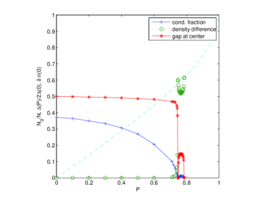
Figure 10: The condensate fraction, density difference, and the order parameter as a function of polarization $P$ obtained for $9000$ atoms. The interaction strength is $(k_{\mathrm{F}}a)^{-1}=-0.50$.

To make connection to experiments Shin et al. (2006) where condensate fractions are measured, we calculate here the condensate fraction for an imbalanced gas. In the case of a balanced Fermi gas the condensate fraction is defined in Campbell (1997); Salasnich et al. (2005) and can be viewed as a measure of the number of condensed pairs which in the extreme BEC limit and at zero temperature is just $N/2\equiv N_{\sigma}.$ For the imbalanced gas, the corresponding number of molecules in the asymptotic BEC limit is the number of minority atoms $N_{\downarrow}.$ It is therefore natural to consider the following normalized condensate fraction

$$N_{0}/N_{\downarrow}=\frac{1}{N_{\downarrow}}\int d^{3}\bm{r}_{1}d^{3}\bm{r}_{2}\left|\langle\Psi_{\uparrow}(\bm{r}_{1})\Psi_{\downarrow}(\bm{r}_{2})\rangle\right|^{2},$$ (22)

for the condensate fraction in the case of $N_{\downarrow}<N_{\uparrow}.$ Figs. 10 and 11 show the density difference, the order parameter at the center of the trap, and the imbalanced condensate fraction from Eq. (22) as function of the polarization for $(k_{\mathrm{F}}a_{s})^{-1}=-0.50$. The critical polarization is roughly $P_{c}=0.78$ and the transition is reflected in a rapid increase in the density difference in the center of the trap. Also the order parameter in the center of the trap drops rapidly. However, as the figures show, there exists a narrow but finite polarization region (in this case for $0.75<P<0.78$) where both the density difference and the gap have non-negligible values in the center of the trap. All data points are for fully converged order parameter and density profiles, satisfying the gap equation with precision of $10^{-6}$. In addition, several points in the plot have been calculated with different initial conditions for the iteration.

The figures are in good qualitative agreement with the experimental condensate fractions Shin et al. (2006), showing the sudden onset of the density difference at the center of the trap when the condensate fraction drops to zero. The core polarized superfluid manifests itself as a weak revival of the condensate fraction as shown in Fig. 12. In other words, a finite condensate fraction co-exists with a finite central density difference. Although the qualitative agreement with the experimental results in Shin et al. (2006) is good, higher experimental accuracy as well as extending our calculations to finite temperatures is needed for quantitative comparison, especially regarding the small window for the core polarized superfluid. Since the condensate fraction is small in the interesting transition region, better signatures of the polarized FFLO-type superfluid may be provided by the central gap, and by the dip in the central density difference as discussed above, provided that temperature dependence is also carefully investigated.

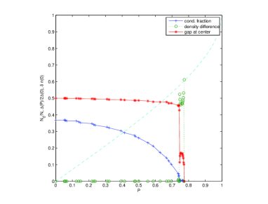
Figure 11: The condensate fraction, density difference, and the order parameter as a function of polarization $P$ obtained for $18000$ atoms. The interaction strength is $(k_{\mathrm{F}}a)^{-1}=-0.50$.

III.4 Contribution of different harmonic oscillator states in pairing

We studied the origin of the oscillations in the BdG order parameter by considering which trap shells (quantum number $n$) are involved in pairing in the center of the trap, i.e. for quantum number $l=0$. As shown in Fig. 13, for zero polarization $P=0$, the pairing involves 0-2 neighboring shells, i.e. is peaked at $n-n^{\prime}=0$, with considerable weight until $n-n^{\prime}=2$ due to strong interactions. For small polarization $P=0.1$ the peak is shifted, but the weight is still very much on the same $n-n^{\prime}$ as for $P=0$, which results to only minor modification of the order parameter profile. However, for large polarization $P\simeq 0.75$, when the oscillations of the order parameter appear also in the center of the trap, the pairing is peaked at nonzero $n-n^{\prime}\sim 11$. Therefore, for large polarizations the state clearly resembles the FFLO state where pairing is predominantly between momentum states $k-k^{\prime}$ determined by the mismatch of the Fermi surfaces (in our example $P\simeq 0.75$ means a mismatch of the Fermi surfaces of about $n-n^{\prime}\sim 11$). We have found that this behavior is not due to small particle number, in contrast, it becomes more clear for larger particle numbers.

IV Conclusions and discussion

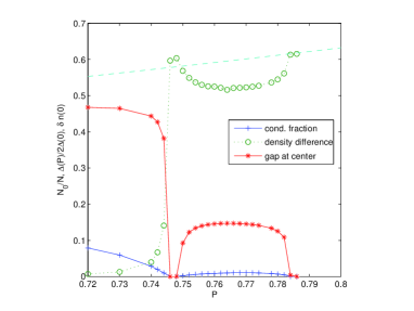
Figure 12: The core polarized superfluid region for $9000$ atoms $(k_{\mathrm{F}}a_{s})^{-1}=-0.50.$

In summary, we have shown that FFLO-type oscillations appear in a trapped polarized Fermi-gas and, for large polarization, extend to the center of the trap thereby realizing a non-BCS superfluid at zero temperature. These results were obtained by BdG calculations using harmonic oscillator eigenstates and particle numbers up to 100000. We have also made a comparison to the results given by local density approximation.

The FFLO-type oscillations of the order parameter appear on the BCS side of the BCS-BEC crossover. When the interaction strength is increased, the polarization required for the existence of the oscillations grows. On the BEC side, no oscillating order parameter was found. The scaling analysis for the penetration depth of the oscillations shows that their characteristic length scale stays constant when the particle number is increased. Therefore the characteristic length scale relative to the atom cloud scale (given by $R_{\mathrm{TF}}$) decreases very slowly, $\propto N^{1/6}$. The features presented here should thus be observable even for condensate sizes corresponding to present-day experiments. RF-spectroscopy was proposed in our earlier work Kinnunen et al. (2006) for detecting the gapless excitations related to the nodes of the order parameter as a signature of the FFLO-type oscillations. The first experiments using RF-spectroscopy in investigating imbalanced gases were recently done Schunck et al. (2007). Moreover, the dip in the central density difference could provide a signature of the core polarized superfluid, as well as the simultaneous measurement of the gap and the density difference in the center of the trap.

The results presented here have an interesting connection to superconductor-ferromagnet interface effects. For future work, it is fascinating to think about the freedom that the ultracold gases offer in terms of designable trapping geometries and other parameters: one should be able to systematically study this kind of effects from the limit of having large superfluid and polarized normal state (“ferromagnet”) regions and a small interface, to the limit where the interface, superfluid, and normal state are all of comparable size and novel mesoscopic phenomena may be found.

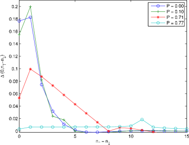
Figure 13: (color online) The gap at the center of the trap (the part of the gap for the quantum number $l=0$ ) as function of the difference in radial quantum number $\Delta n$ for different values of the polarization and for $N=18000.$ For increasing polarization the mainly intra-shell and nearest-neighbor-shell pairing indicated by the central peak (at $P=0$ ) diminishes and a secondary peak appears for large $\Delta n$ which indicate the increasing importance of inter-shell pairing between shell states having an energy separation of order determined by the mismatch of Fermi energies.