All-optical non-demolition measurement of single-hole spin in a quantum-dot molecule

Abstract

We propose an all-optical scheme to perform a non-demolition measurement of a single hole spin localized in a quantum-dot molecule. The latter is embedded in a microcavity and driven by two lasers. This allows to induce Raman transitions which entangle the spin state with the polarization of the emitted photons. We find that the measurement can be completed with high fidelity on a timescale $T\sim 10^{2}$ ps, shorter than the typical $T_{2}$. Furthermore, we show that the scheme can be used to induce and observe spin oscillations without the need of time-dependent magnetic fields.

The capability of encoding and manipulating information at the single-spin level represents a key challenge for semiconductor-based spintronics and quantum-information zutic ; nielsen . A reliable read-out of an individual-spin state is likely to require the measurement to be repeatable. This calls for it to be non-destructive and carried out on timescales shorter than those characterizing spin decoherence meunier ; liu . In this respect, optical manipulation of single carriers in quantum dots (QDs) is specially attractive due to the orders of magnitude separation between optical timescales and those associated to the intrinsic spin dynamics troiani:03 . While most of the attention has been centered in the past on electron spin, it can be argued that hole spin could offer novel alternatives. Along these lines, it has been noted that the decoherence due to hyperfine interactions is suppressed compared to that affecting the electron hrelax .

Here we propose a novel technique to perform a fast and robust non-demolition measurement of single hole spin in a QD-microcavity (MC) system. To illustrate its merit, we also discuss how it could be used to study the spin decoherence with a photon-correlation experiment. The basic idea is to exploit virtual Raman transitions that entangle the spin ($|\!\!\uparrow\rangle$ or $|\!\!\downarrow\rangle$) with the polarization ($\sigma_{+}$ or $\sigma_{-}$) of the photons emitted into the cavity. The semiconductor heterostructure we consider consists of two self-assembled QDs, coherently coupled with each other and embedded in a high-Q optical MC. The quantum-dot molecule (QDM) is doped with an excess hole stinaff , and its lowest-energy trion transition is strongly coupled to a pair of degenerate cavity modes with frequency $\omega_{c}$, damping constant $\kappa$, and polarizations $\sigma_{\pm}$ microp . In the absence of a magnetic field, the ground state of the hole is doubly degenerate and each of the two eigenstates of its spin along the optical axis [$\hat{z}$ in Fig. 1(a)] couples to a different set of trion states. The system’s dynamics is driven by two linearly polarized lasers ($1$ and $2$) with frequencies $\omega_{1}$ and $\omega_{2}$. The photons emitted by the cavity are sorted out with a $\lambda/4$ phase shifter followed by a polarizing beam splitter. The photons with polarization $\sigma_{+}$ ($\sigma_{-}$) are finally sent to the right (left) detector where photocounts $N_{+}$ ($N_{-}$) are recorded. The outcome of the spin ($J_{z}$) measurement is decided based on whether $N_{+}\gtrless N_{-}$, rather than on the presence versus absence of photons in a given mode, and only events in which the measurement outcome satisfies $N_{+}\neq N_{-}$ are post-selected. This strategy makes our scheme intrinsically resilient against photon loss and detector inefficiency. In addition, the asymmetry of the QDM allows to use laser frequencies that are out of resonance with the cavity, and thus to spectrally resolve the output from the light scattered by the heterostructure.

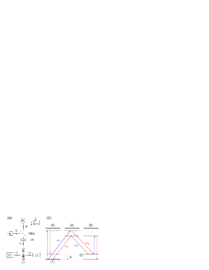
Figure 1: (Color online). (a) Schematic diagram of a possible experimental setup: photocounts $N_{+}$ ($N_{-}$) are recorded at the right (left) detector and the measurement outcome ($|\!\!\uparrow\rangle$ or $|\!\!\downarrow\rangle$) is decided based on whether ($N_{+}\gtrless N_{-}$). (b) Level scheme corresponding to each of the two subspaces, “$+$” and “$-$”. Optical transitions are induced by two lasers (blue arrows) with frequencies $\omega_{1}$ and $\omega_{2}$ linearly polarized along $\hat{x}$, and two degenerate cavity modes (red) with frequency $\omega_{c}$. The scheme relies on Raman transitions between the states $|1\pm\rangle$ and $|2\pm\rangle$, that involve $\sigma_{\pm}$ radiation (solid arrows). All deleterious virtual processes that involve the emission of $\sigma_{\mp}$ photons (an example of which is given by the dotted arrows) are very off-resonant.

A typical QDM is formed by two vertically-stacked QDs. There, the combined effect of strain and effective-mass asymmetry strongly suppresses the hole-state hybridization, while allowing the formation of molecular-like bonding and antibonding states for electrons bester:04 . Thus, we assume that the heavy hole ($J_{z}=\pm 3/2$) remains localized either in the larger dot ($L$) or in the smaller one ($S$), while the electron ($S_{z}=\pm 1/2$) bonding state ($B$) is significantly delocalized over the two. At low temperatures ($T<5$K) and for near resonant interaction with the laser and cavity fields, we can restrict ourselves to a ground-state manifold: $|1\pm\rangle\equiv d^{\dagger}_{\uparrow/\downarrow L}|0\rangle,|2\pm\rangle\equiv d^{\dagger}_{\uparrow/\downarrow S}|0\rangle$, and an excited-state (trion) manifold: $|3\pm\rangle\equiv c^{\dagger}_{\downarrow/\uparrow B}d^{\dagger}_{\uparrow/\downarrow L}d^{\dagger}_{\uparrow/\downarrow S}|0\rangle$, $|4\pm\rangle\equiv c^{\dagger}_{\uparrow/\downarrow B}d^{\dagger}_{\uparrow/\downarrow L}d^{\dagger}_{\downarrow/\uparrow S}|0\rangle$, $|5\pm\rangle\equiv c^{\dagger}_{\uparrow/\downarrow B}d^{\dagger}_{\downarrow/\uparrow L}d^{\dagger}_{\uparrow/\downarrow S}|0\rangle$ [see Fig. 1(b)]. The latter comprises the trion states formed by one heavy-hole per dot and one electron in the bonding state that are optically active, and is separated from $|1\pm\rangle$ by an optical energy difference $\hbar\omega_{T}$. Due to the QDM asymmetry the ground state manifold presents an energy splitting $\hbar\Delta$, which sets the largest energy scale relevant for our purposes.

We note that the interaction with the optical field does not mix the “$+$” and “$-$” states of the QDM. Thus, aside from incoherent spin-flip processes, the dynamics of the system during the spin measurement will satisfy the QND back-action evasion criterion. On the other hand, Raman transitions between the $|1\pm\rangle$ and $|2\pm\rangle$ states [solid arrows in Fig. 1(b)] give rise to a precise correlation between the polarization of the emitted cavity photon ($\sigma_{\pm}$) and the spin orientation ($\uparrow\!\!/\!\!\downarrow$). The cornerstone of the scheme is to choose the laser frequencies so that the two photon resonance condition for these transitions is met – i.e. $\omega_{1}\approx\omega_{c}+\Delta$ and $\omega_{2}\approx\omega_{c}-\Delta$ – while undesired processes, leading to the emission of anticorrelated photons, are kept very off-resonant. A Raman transition mediated by laser $1$ ($2$) transfers the hole from dot $L$ ($S$) to dot $S$ ($L$) and creates a cavity photon. Thus, the combined action of both lasers is equivalent to a cycling transition between $|1\pm\rangle$ and $|2\pm\rangle$ that allows to amplify the single spin to be measured into a many photon state.

In order to study its interaction with the radiation field, we treat the laser driven QDM coupled to the MC as an open quantum system. We apply a time-dependent canonical transformation $\mathcal{O}\rightarrow e^{s(t)}\mathcal{O}e^{-s(t)}$ defined by

$$s(t)=-i\!\!\sum_{\zeta=\pm;\,n=1,2}\left[\tilde{\omega}_{n}t-\frac{(-1)^{n}}{2}\phi(t)\right]\sigma_{nn}^{(\zeta)}-\frac{\tilde{\omega}_{n}t}{2}a_{\zeta}^{\dagger}a_{\zeta}^{\vphantom{{\dagger}}},$$

where: $\sigma_{mn}^{(\zeta)}\equiv|m\zeta\rangle\langle n\zeta|$, $a_{\pm}$ is the annihilation operator for the $\sigma_{\pm}$ polarized cavity mode, $\tilde{\omega}_{1/2}\equiv(3\omega_{1/2}+\omega_{2/1})/4$, and $\phi(t)\!\equiv\!\sum_{n,m}^{2}\int_{0}^{t}\!\mathrm{d}\tau\Omega_{n}^{(m)}(\tau)/[(-1)^{n}\delta_{T}+(3-4\delta_{n,m})\tilde{\Delta}]$. Here we also introduce $\tilde{\Delta}\equiv(\omega_{1}-\omega_{2})/2$, $\delta_{T}\equiv\omega_{1}+\omega_{2}+\Delta-2\omega_{T}$, and the Rabi frequencies $\Omega_{1/2}^{(1)}(t)$ [$\Omega_{1/2}^{(2)}(t)$] for the transitions between $|1/2\pm\rangle$ and the trion states induced by laser $1$ ($2$). In this representation the system’s Hamiltonian is given by $H(t)=H_{0}(t)+V(t)+H_{T}$, with ($\hbar\equiv 1$):

$$H_{0}(t)=\sum_{\zeta=\pm}\left[\delta_{s}-\dot{\phi}(t)/2\right]\left[\sigma_{22}^{(\zeta)}-\sigma_{11}^{(\zeta)}\right]-\delta_{c}a_{\zeta}^{\dagger}a_{\zeta}^{\vphantom{{\dagger}}},$$

$$V(t)= \sum_{\zeta=\pm}\sum_{n=1,2}g_{n}e^{i\frac{(-1)^{n-1}}{2}[\tilde{\Delta}t+\phi(t)]}\left\{\sigma_{3,n}^{(\zeta)}\left[\alpha(t)+a_{\zeta}\right]\right.$$

$$+\left.\sigma_{n+3,n}^{(\zeta)}\left[\alpha(t)+a_{-\zeta}\right]\right\}+\mathrm{H.c.},$$ (1)

and $H_{T}=-\delta_{T}/2\sum_{\zeta=\pm}\sum_{n=3}^{5}\sigma_{nn}^{(\zeta)}$; where we introduce $\alpha(t)\equiv[\Omega_{1}^{(1)}(t)e^{-i\tilde{\Delta}t}+\Omega_{1}^{(2)}(t)e^{i\tilde{\Delta}t}]/2g_{1}$, the detunings $\delta_{s}\equiv(\Delta-\tilde{\Delta})/2$, $\delta_{c}\equiv(\omega_{1}+\omega_{2})/2-\omega_{c}$, and the QDM-MC couplings $g_{1/2}\!>\!0$. In addition there are dissipative contributions associated to the cavity losses and to the spontaneous emission of the trion into leaky modes. Their respective Liouvillians, $\mathcal{L}_{C}$ and $\mathcal{L}_{T}(t)$, are of the Lindblad form with collapse operators given by: $\sqrt{\kappa}a_{\pm}$ and $c_{\pm}(t)=\sqrt{\Gamma}\sum_{n}^{2}(g_{2}/g_{1})^{n-1}e^{i(-1)^{n}[\tilde{\Delta}t+\phi(t)]/2}[\sigma_{n,3}^{(\pm)}+\sigma_{n,n+3}^{(\mp)}]$. Here $\Gamma$ is the spontaneous-emission rate to the state $|1\pm\rangle$.

In the virtual-Raman regime of interest, $|\delta_{T}|\lesssim|\tilde{\Delta}|$, with the latter much larger than all the other frequency scales in $H(t),\mathcal{L}_{T/C}$. This warrants an adiabatic elimination of the trion-ground state coherences cohen ; gardiner . To this effect, we decompose the density matrix of the QDM-MC system ($\rho$) into a relevant part $\mathbb{P}\rho=P_{0}\rho P_{0}+P_{T}\rho P_{T}$ and an irrelevant one $[\mathbb{I}-\mathbb{P}]\rho(t)$ – where $P_{0}$ ($P_{T}$) is the projector onto the ground state (trion) manifold. We subsequently eliminate the irrelevant part, introduce a formal parameter $\lambda$ such that $\delta_{T}\to\lambda\delta_{T}$ and $\tilde{\Delta}\to\lambda\tilde{\Delta}$, and consider the asymptotic expansion of $\mathbb{P}\dot{\rho}$ as $\lambda\to\infty$ gardiner . To the lowest non-trivial order ($1/\lambda$), $\mu\equiv P_{0}\rho P_{0}$ obeys a closed evolution generated by $\mathcal{L}_{C}$ and the effective Hamiltonian

$$H_{\mathrm{eff}}= \sum_{\zeta=\pm}\delta_{s}\sigma_{z}^{(\zeta)}-\left\{\delta_{c}-\Delta_{c}-\Delta_{s}\left[\sigma_{z}^{(\zeta)}+\sigma_{z}^{(-\zeta)}\right]\right\}a_{\zeta}^{\dagger}a_{\zeta}^{\vphantom{{\dagger}}}$$

$$+\!\left\{\left[\frac{g_{2}|\Omega_{1}^{(1)}(t)|}{\delta_{T}+\tilde{\Delta}}\sigma_{+}^{(\zeta)}+\frac{g_{1}|\Omega_{2}^{(2)}(t)|}{\delta_{T}-\tilde{\Delta}}\sigma_{-}^{(\zeta)}\right]a_{\zeta}^{\dagger}+\mathrm{H.c.}\!\right\},$$

where we have introduced Pauli matrix notation for the orbital pseudospin $\sigma_{+}^{(\pm)}\equiv\sigma_{21}^{(\pm)}$, $\Delta_{c/s}\equiv g_{2}^{2}/(\delta_{T}+\tilde{\Delta})\pm g_{1}^{2}/(\delta_{T}-\tilde{\Delta})$, and we have chosen $\Omega_{1/2}^{(1/2)}(t)/|\Omega_{1/2}^{(1/2)}(t)|=e^{\mp i\phi(t)}$. On the other hand we find that the spontaneous emission only contributes to order $1/\lambda^{2}$. In terms of the physical parameters this corresponds to a correction to the evolution generated by $H_{\mathrm{eff}}$ of relative order $\Gamma/\Delta\ll 1$. The above treatment is valid provided $|\Omega_{1}^{(1/2)}(t)|^{2}\ll(n|\tilde{\Delta}|-|\delta_{T}|)^{2}$ and $\kappa,\Gamma,|\delta_{c/s}|,|\dot{\Omega}_{1}^{(1/2)}(t)/\Omega_{1}^{(1/2)}(t)|\ll|n|\tilde{\Delta}|-|\delta_{T}||$ are satisfied for $n=1,3$; where we assume $g_{2}<g_{1}<|\Omega_{1}^{(1/2)}(t)|/2$ and that the typical cavity occupancies are at most of order unity. We take laser and cavity frequencies so that $\delta_{s}\!=\!0$, $\delta_{c}\!=\!\Delta_{c}$, $\Delta_{s}\!=\!0$. The asymmetry of the molecule ensures $|n|\tilde{\Delta}|-|\delta_{T}||\sim\Delta$ ($n\!\!=\!\!1,3$). The relative intensities of the two lasers are chosen so that the coefficients of $\sigma^{(\pm)}_{+}$ and $\sigma^{(\pm)}_{-}$ are equal. This yields $\tilde{H}_{\mathrm{eff}}=-\tilde{\Omega}(t)/2\sum_{\zeta}\sigma^{(\zeta)}_{x}(a_{\zeta}^{\dagger}+a_{\zeta}^{\vphantom{{\dagger}}})$ with $\tilde{\Omega}(t)=|\Omega_{1}^{(1)}(t)|(g_{1}^{2}-g_{2}^{2})/g_{2}\Delta$. The lasers are switched on at $t=0$ so that for negative times $\tilde{\Omega}(t)=0$ with the cavity modes in the vacuum.

As will be borne out below, to analyze the measurement process it is useful to consider the time evolution conditioned upon having no photocounts detected gardiner : $\dot{\mu}\!=\!\sum_{\zeta=\pm}-i[\tilde{H}_{\mathrm{eff}},\mu]+\mathcal{L}_{C}^{(\zeta)}(\eta)\mu\,$ with $\mathcal{L}^{(\zeta)}_{C}(\eta)\mu=(\kappa/2)[2(1-\eta)a_{\zeta}^{\vphantom{{\dagger}}}\mu a_{\zeta}^{\dagger}-\{a_{\zeta}^{\dagger}a_{\zeta}^{\vphantom{{\dagger}}},\mu\}]$. Here $\eta$ is the collection efficiency times the efficiency of the detectors and for $\eta\!=\!0$ one recovers the standard time evolution. This equation for $\mu(t)$ has the following solution:

$$\mu(t)= \sum_{\zeta=\pm}\sum_{\nu=0}^{3}e^{-\xi_{\nu}\kappa P(t)}e^{-ip(t)\sigma^{(\zeta)}_{x}\left(a_{\zeta}^{\dagger}+a_{\zeta}^{\vphantom{{\dagger}}}\right)}|0\rangle\langle 0|_{+}$$

$$\otimes|0\rangle\langle 0|_{-}\otimes\frac{\mathrm{Tr}[\sigma^{(\zeta)}_{\nu}\mu(0)]}{2}\sigma^{(\zeta)}_{\nu}e^{ip(t)\sigma^{(\zeta)}_{x}\left(a_{\zeta}^{\dagger}+a_{\zeta}^{\vphantom{{\dagger}}}\right)}\,$$ (2)

where $\xi_{0/1}\equiv\eta$, $\xi_{2/3}\equiv 2-\eta$, and $P(t)=\int_{0}^{t}\!\mathrm{d}\tau p(\tau)^{2}$ with $p(t)$ satisfying: $2\dot{p}=-\tilde{\Omega}(t)-\kappa p$, $p(0)=0$. Here $|0\rangle\langle 0|_{\pm}$ are the vacuum states for the cavity modes, $\sigma^{(\zeta)}_{0}\equiv\sigma^{(\zeta)}_{11}+\sigma^{(\zeta)}_{22}$, and $\sigma^{(\zeta)}_{\nu}$ with $\nu\!>\!0$ correspond to the Pauli matrices. The profiles of the laser pulses are chosen so that $\tilde{\Omega}(t)=\tilde{\Omega}_{0}[e^{-8(t/t_{s}-1)^{2}}\Theta(t_{s}-t)+\Theta(t-t_{s})]$, where $t_{s}$ is a switch-on time. We choose $1/\Delta\ll t_{s}\ll 1/\tilde{\Omega}_{0}$ so that $t_{s}\tilde{\Omega}_{0}$ is a small parameter and one can keep only the zeroth order. This corresponds to $\kappa P(t)=p_{0}^{2}f[\kappa t/2]$ where $f[x]\equiv 2x+1-(2-e^{-x})^{2}$ and $p_{0}\equiv\tilde{\Omega}_{0}/\kappa$, which specifies $\mu(t)$.

If we now consider in Eq. (All-optical non-demolition measurement of single-hole spin in a quantum-dot molecule) $\eta=0,\,t\to\infty$ we obtain the steady state to which the system converges starting from a given initial condition for the hole $\rho_{h}$:

$$\mu_{\mathrm{ss}}=\!\!\sum_{\xi=\pm}\!|\!\!\uparrow\!\xi\rangle\langle\uparrow\!\xi|\rho_{h}|\!\!\uparrow\!\xi\rangle\langle\uparrow\!\xi|\!\otimes\!|\!-\!\xi ip_{0}\rangle\langle-\xi ip_{0}|_{\scriptscriptstyle+}\!\otimes\!|0\rangle\langle 0|_{\scriptscriptstyle-}$$

$$+|\!\!\downarrow\!\xi\rangle\langle\downarrow\!\xi|\rho_{h}|\!\!\downarrow\!\xi\rangle\langle\downarrow\!\xi|\!\otimes\!|0\rangle\langle 0|_{\scriptscriptstyle+}\!\otimes\!|\!-\!\xi ip_{0}\rangle\langle-\xi ip_{0}|_{\scriptscriptstyle-}$$ (3)

Here we have defined $|\!\!\uparrow\!\!/\!\!\downarrow\!\xi\rangle\equiv(|2\pm\rangle+\xi|1\pm\rangle)/\sqrt{2}$ and introduced the cavity coherent states $|\lambda\rangle_{\pm}$. We note the perfect correlation between the initial state of the spin and the polarization of the cavity mode that does not remain in the vacuum, and its independence from the initial orbital state of the carrier. In addition we find that the eigenstates of the orbital pseudospin $\sigma_{x}$ become correlated with the phase quadratures of the cavity fields. Thus if homodyne detection is performed for both circular polarizations one can also measure the orbital state of the hole in the $|2\pm\rangle\pm|1\pm\rangle$ basis.

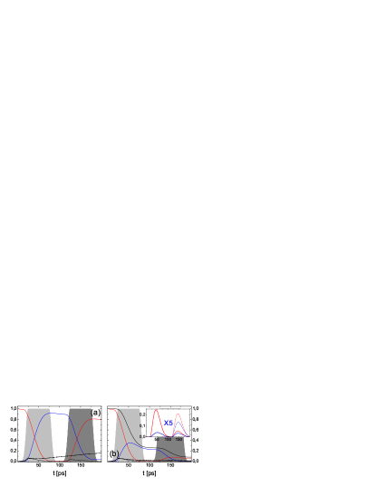
Figure 2: (Color online). Simulated time evolution of the unconditional (a) and conditional (b) density matrices under the effect of two consecutive laser pulses, with frequencies $\omega_{1}$ (light gray area) and $\omega_{2}$ (dark gray). The curves show the occupations of: state $|1+\rangle$ (red line), state $|2+\rangle$ (blue), the trion manifold $|n\!>\!2\,\,\pm\rangle$ (black dotted), and the “$-$” subspace (black dashed). The solid black line in panel (b) corresponds to $\mathrm{Tr}\{\rho(t)\}$. Figure inset: photon occupations $\langle a^{\dagger}_{\zeta}(t)a_{\zeta}(t)\rangle$ for $\zeta=+$ (red) and $\zeta=-$ (blue, $\times 5$), in the conditional (solid lines) and unconditional (dotted) cases. The values of the parameters are: $g_{1,2}=0.2,0.15\,$meV, $\Omega_{1}^{(1)}(t_{s})=0.4\,$meV, $\Omega_{2}^{(1)}(t_{s})=0.3\,$meV, $\kappa=0.1\,$ps^-1, $\Gamma_{S}=1\,$ns^-1, $\Gamma=2\,$ns^-1; (b) $\eta=0.75$.

To assess the performance of the proposed measurement strategy [Fig. 1(a)] one can take the signal output density matrix for the spin ralph as $\rho_{\mathrm{\,O}}\!=\!\sum_{\zeta}\langle\hat{P}_{\zeta}\rangle\mathrm{Tr}_{\mathrm{orb}}\{\sigma^{(\zeta)}_{0}\}/(2\sum_{\zeta}\langle\hat{P}_{\zeta}\rangle)$, where the orthogonal projectors $\hat{P}_{\pm}(T)=\hat{S}(T)[\hat{S}(T)\pm 1]/2$ correspond to the events $N_{+}(T)\gtrless N_{-}(T)$. Here $\hat{S}(T)\equiv\mathrm{sgn}[\hat{N}_{+}(T)-\hat{N}_{-}(T)]$ and $T$ is the total time over which the photocounts are integrated. The signal input density matrix can be defined as $\rho_{\mathrm{\,I}}\!\!=\!\!\mathrm{Tr}_{\mathrm{orb}}\{\sum_{\zeta}\sigma^{(\zeta)}_{0}\rho_{h}\sigma^{(\zeta)}_{0}\}$. Then, the quality of the measurement can be characterized by $F^{\mathrm{Min}}_{M}(T)=\mathrm{Min}\{F[\rho_{\mathrm{\,O}}(T),\rho_{\mathrm{\,I}}]\}|_{\rho_{\mathrm{\,I}}}$ ralph where $F$ is the square of the standard fidelity nielsen . The probability of measurement “failure” ($N_{+}=N_{-}$) is given by $\langle 1-\hat{S}(T)^{2}\rangle$. In all the regimes we will study below, either the deviations from $H_{\mathrm{eff}}$ will be small enough to guarantee that the emission of anticorrelated photons remains improbable or the emission of more than one photon will have low probability. It is straightforward to argue that under these circumstances, it is permissible to redefine $\langle\hat{P}_{\pm}\rangle\to\kappa\eta\int_{0}^{T}\!\mathrm{d}t\,\langle a^{{\dagger}}_{\pm}(t)a_{\pm}^{\vphantom{{\dagger}}}(t)\rangle|_{\eta}$, which is the probability that the first photon detected has polarization $\sigma_{\pm}$.

We analyze now the physical limits for the measurement time $T$. Naturally, there will be non-trivial spin dynamics neglected in $H(t)$ – e.g. spin decoherence – that will set an upper limit for $T$. On the other hand, a lower limit for $T$ is set by the requirement that $F^{\mathrm{Min}}_{M}(T)$ and $\langle\hat{S}(T)^{2}\rangle$ be close to unity. Within the above approximations we have $F^{\mathrm{Min}}_{M}(T)=1$ and the measurement can be considered completed when the probability of not having detected a photon falls below $\epsilon\ll 1$. From Eq. (All-optical non-demolition measurement of single-hole spin in a quantum-dot molecule) it follows that this probability evolves as $\mathrm{Tr}\{\mu(t)\}=e^{-\eta\kappa P(t)}$. This implies $T=(-\ln\epsilon/\eta\tilde{\Omega}_{0}^{2}y)^{1/2}f^{-1}[y]$ with $y=-\kappa^{2}\ln\epsilon/\eta\tilde{\Omega}_{0}^{2}$. Numerical optimization then yields $T_{\mathrm{min}}\approx 3(-\ln\epsilon/\eta)^{1/2}/\tilde{\Omega}_{\mathrm{max}}$ for $\kappa_{\mathrm{opt}}\approx\sqrt{\eta/\ln(1/\epsilon)}\tilde{\Omega}_{\mathrm{max}}$, with $\tilde{\Omega}_{\mathrm{max}}$ a maximum value of $\tilde{\Omega}_{0}$ allowed by the conditions we discussed needed for the validity of $H_{\mathrm{eff}}$. If $\kappa_{\mathrm{opt}}$ cannot be reached the optimum is to take instead the lowest possible $\kappa$. Experimental developments prompt us to consider as a typical example: $\eta=0.75$, $\hbar\Delta=2$meV, $\hbar g_{1}=0.2$meV, $\hbar\kappa=0.05$meV and $g_{1}/g_{2}=\sqrt{3}$; which lead to $T\approx 200$ps for $\epsilon\sim 10^{-2}$, with $\hbar\Omega_{1}^{(1)}(t_{s})=0.4$meV.

The above analysis of the system’s evolution and the resulting timescales for $T$, that follow from Eq. All-optical non-demolition measurement of single-hole spin in a quantum-dot molecule, rely on the simultaneous switch-on (SSO) of the two lasers. An alternative approach consists in applying an alternating sequence of non-overlapping pulses with frequencies $\omega_{1},\omega_{2},\omega_{1},\omega_{2},\dots$ (see Fig. 2). In this case, each pulse triggers the emission of a single photon. We find that an analysis based on $H_{\mathrm{eff}}$, analogous to the one performed for the SSO strategy, allows to establish $\kappa_{\mathrm{opt}}\approx 2\tilde{\Omega}_{\mathrm{max}}$, and that $T_{\mathrm{min}}\sim 1/\eta\tilde{\Omega}_{\mathrm{max}}$ for the complete pulse sequence. Thus, though the SSO strategy is preferable for low $\eta$, in the range we will focus on ($\eta\gtrsim 0.7$) the timescales $T$ for the two approaches are comparable. On the other hand, the “pulsed” scenario directly relates to photon-correlation experiments, that allow to probe the spin’s “intrinsic” dynamics.

In the following, we numerically solve the complete conditional master equation for the QDM-MC system. The unitary part of the evolution is induced by the Hamiltonian $H(t)$ (see Eq. All-optical non-demolition measurement of single-hole spin in a quantum-dot molecule). The dissipative contribution, instead, is given by $\mathcal{L}_{C}^{(+)}(\eta)+\mathcal{L}_{C}^{(-)}(\eta)+\mathcal{L}_{T}(t)+\mathcal{L}_{S}$, where the collapse operators of the Liouvillian $\mathcal{L}_{S}$, accounting for the spin-flip process, are $\sqrt{\Gamma_{S}}\sigma_{\uparrow\downarrow}$ and $\sqrt{\Gamma_{S}}\sigma_{\uparrow\downarrow}^{\dagger}$, with $\sigma_{\uparrow\downarrow}\equiv\sum_{n=1}^{2}|n+\rangle\langle n\!-\!|$. In Fig. 2 we plot the system’s time evolution under the effect of two consecutive laser pulses (shaded gray areas) for both the unconditional [$\eta=0$, panel (a)] and the conditional case [$\eta\neq 0$, panel (b)]. The first pulse essentially induces a population transfer from the initial state $|1+\rangle$ (blue line) to $|2+\rangle$ (red). The second Raman transition, due to the following laser pulse, drives the hole back to dot $L$. While the overall occupation of the excitonic manifold (black dotted lines) is kept negligible throughout the process, $\rho$ suffers a population leakage to subspace “$-$” (dashed lines), which is responsible for the finite probability of emitting a $\sigma_{-}$ photon (blue lines in the inset). We note that these numerical simulations clearly support the approximations underpinning the effective Hamiltonian $H_{\mathrm{eff}}$. The merits of the measure ultimately depend on the occupations of the cavity mode. In particular, we find that the final probability of having recorded no photocounts ($\mathrm{Tr}\{\rho\}|_{\eta\neq 0}$) falls below $0.1$, while $\langle\hat{P}_{+}\rangle=0.71\,(0.87)$ and $\langle\hat{P}_{-}\rangle=0.027\,(0.048)$ after one pulse (two pulses), yielding $F^{\mathrm{Min}}_{M}=0.963\,(0.947)$. The repetition of the measurement while decreasing $\mathrm{Tr}\{\rho\}|_{\eta\neq 0}$, slightly worsens the fidelity. This is because the repetition time is not sufficiently short compared to $1/\Gamma_{S}$.

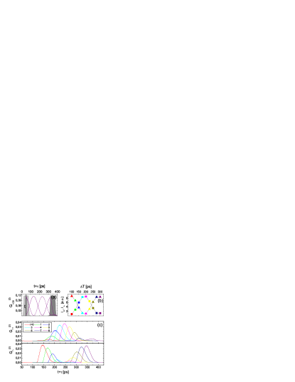
Figure 3: (Color online). (a) Correlation functions $G^{(2)}_{+,2\pm}(t,t+\tau)$. The pulse from laser 1 (light gray) and the detection of a $\sigma_{+}$ photon at time $t$ (vertical black line) initialize the spin state, setting in damped oscillations between states $|2+\rangle$ (dotted curve) and $|2-\rangle$ (solid). The pulse from laser 2 (dark gray, $\Delta T=300\,$ps), probes the spin evolution. (b) Time integrals of $G^{(2)}_{++}$ (squares) and $G^{(2)}_{+-}$ (triangles), for different values of the delay between the two pulses: $\Delta T=(100+25\,i)\,$ps, with $i=0,\dots,8$ (see the legend). (c) Correlation functions $G^{(2)}_{+\beta}(t,t+\tau)$, for $\beta=+$ (upper panel) and $\beta=-$ (lower panel), as a function of $t+\tau$ ($t=50$ ps). $B_{x}=0.5$ T.

The non-destructive nature of our measurement scheme turns it into an ideal means to probe the spin’s dynamics. In particular, the polarization correlations between two photons detected at times $t$ and $t+\tau$ can be used to investigate the evolution that the spin undergoes in such time interval. As above, the system’s state is driven by a sequence of two non-overlapping laser pulses, with frequencies $\omega_{1}$ and $\omega_{2}$ [Fig. 3(a)]. The first pulse (light gray area) induces a Raman transition which displaces the hole from dot $L$ to dot $S$. The cases where a $\sigma_{+}$ photon is detected at a given time $t$ (vertical black line) are post-selected: this first measurement (approximately) projects $\rho$ onto the $|2+\rangle$ state, thus initializing the spin to a pure state. A tunable time-interval $\Delta T$ follows, during which the spin freely evolves under the effect of the spin-flip process, and eventually of an applied magnetic field $\mathbf{B}$. The corresponding time-evolution, conditioned upon having detected a photon at time $t$, is given by the second-order correlation functions $G^{(2)}_{\zeta,n\beta}(t,t+\tau)=\langle\,a_{\zeta}^{\dagger}(t)\,\sigma_{nn}^{(\beta)}(t+\tau)\,a_{\zeta}(t)\,\rangle$, with $\zeta,\beta=\pm$. Finally, the second laser pulse (dark gray) probes the spin state, while displacing the carrier back to dot $L$. If the magnetic field is applied in the $z$ direction, the polarization correlations between the first and the second detected photons, given by $G^{(2)}_{\zeta\beta}(t,t+\tau)=\langle\,a_{\zeta}^{\dagger}(t)\,a_{\beta}^{\dagger}(t+\tau)\,a_{\beta}(t+\tau)\,a_{\zeta}(t)\,\rangle$, only reflect the effect of $\mathcal{L}_{S}$, allowing to infer the value of $T_{1}=1/\Gamma_{S}$. If $\mathbf{B}\!\!\parallel\!\!\hat{x}$ instead Zeeman , $J_{z}$ is no longer a constant of motion of $H(t)$, and its time-evolution will consist of damped oscillations between the states $|2+\rangle$ and $|2-\rangle$ (solid and dotted curves, respectively). Due to the high fidelity of the initializing measurement, the initial conditions do not play here a crucial role. As the energy splitting induced by $\mathbf{B}$ is small compared to $k_{B}T$, we take $\rho_{h}=(|1+\rangle\langle 1\!+\!|+|1-\rangle\langle 1\!-\!|)/2$. In Fig. 3(c) we plot $G^{(2)}_{\zeta\beta}(t,t+\tau)$, for $\zeta=+$ and $\beta=\pm$ (upper and lower panels, respectively), and for different values of $\Delta T$. The time integrals of these functions $I_{\zeta\beta}=\int G^{(2)}_{\zeta\beta}(t,t+\tau)\,d\tau$ clearly show an oscillatory behavior as a function of $\Delta T$ [Fig. 3(b)]. The free damped oscillations we observe reflect the decay of the initial coherence between the eigenstates of $J_{x}$, and thus would allow to infer the $T_{2}$ for a transverse field.

In conclusion, we have proposed an all-optical robust scheme to perform a QND measurement of a single hole spin in sub-nanosecond timescales. Furthermore, we have pointed out how in the presence of a static magnetic field photon correlation experiments would allow to study the spin decoherence. Beyond measurement, the entanglement between the carrier and the photon could enable generation of EPR pairs. In the case of correlations with the phase quadratures [Eq.(All-optical non-demolition measurement of single-hole spin in a quantum-dot molecule)] one could also envisage the generation of Schrödinger cat states of the emitted light. Finally, the same system could be operated in a continuous measurement regime with the spin-flip processes inducing quantum jumps in the output.

We thank J.C. Cuevas and J. Eschner for discussions. Work supported by the Spanish MEC under the contracts MAT2005-01388 and NAN2004-09109-C04-4, by CAM under Contract S-0505/ESP-0200, and by the EU within the RTN’s COLLECT and CLERMONT2.

References

• (1) I. Z̆utić, et al., Rev. Mod. Phys., 76, 323 (2004).
• (2) M. A. Nielsen and I. L. Chuang, Quantum Computation and Quantum Information (Cambridge University Press, Cambridge, England, 2000).
• (3) T. Meunier, et al., cond-mat/0603794.
• (4) R.-B. Liu, et al., Phys. Rev. B. 72, 81306(R) (2005).
• (5) F. Troiani, et al., Phys. Rev. Lett., 90, 206802 (2003).
• (6) D. V. Bulaev and D. Loss, Phys. Rev. Lett. 95, 76805 (2005).
• (7) E. A. Stinaff, et al., Science, 311, 636 (2006).
• (8) A micropillar structure affords a physical realization. See, e.g., J.P. Reithermaier et al., Nature, 432, 197 (2004).
• (9) G. Bester, et al., Phys. Rev. Lett. 93, 47401 (2004).
• (10) C. W. Gardiner and P. Zoller, Quantum Noise (Springer-Verlag, Berlin, 2004).
• (11) C. Cohen-Tannoudji, J. Dupont-Roc, and G. Grynberg, Atom-Photon Interactions (Wiley, US, 1992).
• (12) For the effective spin Hamiltonian $H_{B}$ and typical parameters, see: H. W. van Kesteren, et al., Phys. Rev. B. 41, 5283 (1990); M. Bayer, et al., Phys. Rev. B. 61, 7273 (2000). Here, we also include the dark states $|6\pm\rangle\equiv c^{\dagger}_{\uparrow/\downarrow B}d^{\dagger}_{\uparrow/\downarrow L}d^{\dagger}_{\uparrow/\downarrow S}|0\rangle$.
• (13) T. C. Ralph, et al., Phys. Rev. A 73, 12113 (2006).