Critical aging of Ising ferromagnets relaxing from an ordered state

Abstract

We investigate the nonequilibrium behavior of the $d$-dimensional Ising model with purely dissipative dynamics during its critical relaxation from a magnetized initial configuration. The universal scaling forms of the two-time response and correlation functions of the magnetization are derived within the field-theoretical approach and the associated scaling functions are computed up to first order in the $\epsilon$-expansion ($\epsilon=4-d$). Aging behavior is clearly displayed and the associated universal fluctuation-dissipation ratio tends to $X^{\infty}=\frac{4}{5}[1-(\frac{73}{480}-\frac{\pi^{2}}{80})\epsilon+O(\epsilon^{2})]$ for long times. These results are confirmed by Monte Carlo simulations of the two-dimensional Ising model with Glauber dynamics, from which we find $X^{\infty}_{\rm MC}=0.73(1)$. The crossover to the case of relaxation from a disordered state is discussed and the crossover function for the fluctuation-dissipation ratio is computed within the Gaussian approximation.

I Introduction

The dynamics of statistical systems close to critical points has been the subject of intensive theoretical and experimental investigations in the last three decades, during which mainly equilibrium properties have been studied in detail. As in the case of static properties, the presence of a nearby critical point greatly facilitate the study of dynamical behavior. In fact, upon approaching a second-order phase transition some of the relevant features of the dynamics (at length and time scales much larger than the microscopic ones) are determined only by the fluctuations of a suitable order parameter and they become to some extent independent of the actual microscopic details of the system (universality). In turn, this allows a quantitative characterization of the dynamical behavior within the various universality classes grouping together the microscopically different systems which display the same critical behavior. This can be usually done to an extent that is in general well out of reach for the general case of non-critical dynamics.

Critical dynamics provides also a simple instance of slow collective evolution. Statistical systems with slow dynamics have recently attracted considerable theoretical and experimental interest, in view of the rich scenario of phenomena they display: Dramatic slowing down of relaxation processes, hysteresis, memory effects, etc. After a perturbation a system with slow dynamics does not generically achieve equilibrium even for long times and its dynamics is neither invariant under time translations nor under time reversal, as it should be in thermal equilibrium. During this never-ending relaxation aging occurs: Two-time quantities such as response and correlation functions depend on the two times $s$ and $t>s$ not via $t-s$ only and their decays as functions of $t$ are slower for larger $s$. At variance with one-time quantities (e.g., the order parameter) – converging to asymptotic values in the long-time limit – two-time quantities clearly bear the signature of aging.

Aging was known to occur in disordered and complex systems (see, e.g., Ref. [1]) and only in the last ten years attention has been focused on simpler systems such as critical ones, whose universal features can be rather easily investigated by using different methods and which might provide insight into more general cases [2] (see also Ref. [3] for a pedagogical introduction). Indeed, consider a system with a critical point at temperature $T_{c}$, order parameter $\varphi({\bf x},t)$, and prepare it in some initial configuration (which might correspond to an equilibrium state at a given temperature $T_{0}$). At time $t=0$ bring the system in contact with a thermal bath of temperature $T_{b}$($\neq T_{0}$). The ensuing relaxation process is expected to be characterized by some equilibration time $t_{\rm eq}(T_{b})$ such that for $t\gg t_{\rm eq}(T_{b})$ equilibrium is attained and the dynamics is stationary and invariant under time reversal, whereas for $0<t\ll t_{\rm eq}(T_{b})$, the evolution depends on the specific initial condition. Upon approaching the critical point $T_{b}=T_{c}$ the equilibration time diverges and therefore equilibrium is never achieved. To monitor the time evolution we consider the average order parameter $M(t)=\langle\varphi({\bf x},t)\rangle$ (translational invariance in space is assumed), the time-dependent correlation function of the order parameter $C_{\bf x}(t,s)=\langle\varphi({\bf x},t)\varphi({\bf 0},s)\rangle$, where $\langle\ldots\rangle$ stands for the mean over the stochastic dynamics, and the linear response (susceptibility) $R_{\bf x}(t,s)$ to an external field. $R_{\bf x}(t,s)$ is defined by $R_{\bf x}(t,s)=\delta\langle\varphi({\bf x},t)\rangle/\delta h(s)$, where $h$ is a small external field, conjugate to $\varphi({\bf x}={\bf 0},s)$ (e.g., if $\varphi$ is a magnetic order parameter, $h$ is the magnetic field), applied at time $s>0$ at the point ${\bf x}={\bf 0}$. Note that causality implies $R_{\bf x}(t,s>t)=0$ and that $C_{\bf x}(t,s)=C_{\bf x}(s,t)$ in the bulk. According to the general picture of the relaxation process, one expects that for $t>s\gg t_{\rm eq}(T_{b})$, $C_{\bf x}(t,s)=C^{\rm eq}_{\bf x}(t-s)$ and $R_{\bf x}(t,s)=R^{\rm eq}_{\bf x}(t-s)$ where $C^{\rm eq}_{\bf x}$ and $R^{\rm eq}_{\bf x}$ are the corresponding equilibrium quantities, related by the fluctuation-dissipation theorem (FDT)

$$R^{\rm eq}_{\bf x}(\tau>0)=-\frac{1}{T_{b}}\frac{{\rm d}C^{\rm eq}_{\bf x}(\tau)}{{\rm d}\tau}\;,$$ (1)

where the temperature is measured in unit of the Boltzmann’s constant. The FDT suggests the definition of the so-called fluctuation-dissipation ratio (FDR) [4, 5]:

$$X_{\bf x}(t,s)=\frac{T_{b}\,R_{\bf x}(t,s)}{\partial_{s}C_{\bf x}(t,s)}\;,$$ (2)

where we assume $t>s$. According to the previous picture for $t>s\gg t_{\rm eq}(T_{b})$ the FDT yields $X_{\bf x}(t,s)=1$. This is not generically true in the aging regime. The asymptotic value of the FDR

$$X^{\infty}=\lim_{s\to\infty}\lim_{t\to\infty}X_{{\bf x}=0}(t,s)$$ (3)

is a very useful quantity in the description of systems with slow dynamics, since $X^{\infty}=1$ whenever the aging evolution is interrupted and the system crosses over to equilibrium dynamics, i.e., $t_{\rm eq}(T_{b})<\infty$. Conversely $X^{\infty}\neq 1$ is a signal of an asymptotic non-equilibrium dynamics. Moreover $X^{\infty}$ can be used to define an effective non-equilibrium temperature $T_{\rm eff}=T/X^{\infty}$, which might have some features of the temperature of an equilibrium system, e.g., controlling the direction of heat flows and acting as a criterion for thermalization [6]. Within the field-theoretical approach to critical dynamics it is more convenient to focus on the behavior of observables in momentum space. Accordingly hereafter we mainly consider the momentum-dependent response $R_{\bf q}(t,s)$ and correlation $C_{\bf q}(t,s)$ functions, defined as the Fourier transform of $R_{\bf x}(t,s)$ and $C_{\bf x}(t,s)$, respectively. In momentum space it is natural to introduce a quantity that, just like $X_{\bf x}(t,s)$, “gauges” the distance from equilibrium evolution [7]:

$${\cal X}_{\bf q}(t,s)=\frac{T_{b}R_{\bf q}(t,s)}{\partial_{s}C_{\bf q}(t,s)}\;.$$ (4)

Note that ${\cal X}_{\bf q}(t,s)$ is not the Fourier transform of $X_{\bf x}(t,s)$. The long-time limit

$${\cal X}^{\infty}_{{\bf q}=0}\equiv\lim_{s\rightarrow\infty}\lim_{t\rightarrow\infty}{\cal X}_{{\bf q}=0}(t,s)\;$$ (5)

has been used to define an effective temperature, in analogy with $X^{\infty}$. Interestingly, it has been argued that $X^{\infty}={\cal X}^{\infty}_{{\bf q}=0}$ [7] (see also Ref. [8]). However, for quenches to the critical point ${\cal X}^{\infty}_{{\bf q}=0}$ (and therefore $X^{\infty}$) depends on the specific choice of the quantity which $R_{\bf q}$ and $C_{\bf q}$ refer to [10] and therefore it would be difficult to assign a sound physical meaning to $T_{\rm eff}$ defined from $X^{\infty}$ (see also [9]).

We shall consider here the universal aspects of one of the simplest dynamic universality class: Pure relaxation (Model A in the notion of Ref. [11]) within the Ising (static) universality class. As we shall discuss later on, the lattice Ising model with Glauber dynamics belongs to it. In spite of its simplicity the non-equilibrium behavior of this model has been investigated in some detail only recently. In particular, earlier works focussed primarily on general scaling properties of the non-linear relaxation [12, 13] close to $T_{c}$ and on the equation of motion describing the dynamics of the order parameter in the presence of time-dependent external fields [14, 15]. Two-time quantities such as correlation and response functions were not discussed explicitly beyond equilibrium [14], although the non-equilibrium behavior of $R_{{\bf q}=0}(t,s)$ was implicitly encoded in the equation of motion computed in Refs. [14, 15]. A more careful analysis of the relaxation process from a given initial (non-equilibrium) state revealed the presence of an additional stage of relaxation with universal features [16, 17] (characterized by the initial-slip exponent $\theta$, cf. Sec. III) which was previously overlooked. The general analysis of Refs. [16, 17] provided the scaling functions for generic multi-time quantities and in particular for the order parameter $M(t)$ and for the two-time quantities $R_{\bf x}(t,s)$ and $C_{\bf x}(t,s)$. On the other hand there was no explicit analysis of the resulting aging behavior at the critical point, which has been later carried out in Ref. [5, 7, 18, 19, 20, 10] by computing the two-time response and correlation functions for the case of a relaxation from an initially disordered state with vanishing order parameter (corresponding to a quench from high temperature to the critical point). In particular it has been shown that $X^{\infty}=0$ for quenches below $T_{c}$, whereas $X^{\infty}$ is a universal amplitude ratio for quenches to $T_{c}$, as pointed out by Godrèche and Luck [18]. Accordingly it is possible to take advantage of this universality by computing $X^{\infty}$ within the field-theoretical approach to critical dynamics. For the Ising universality class with purely relaxational dynamics this analysis leads to $X^{\infty}(d=3)=0.429(6)$, $X^{\infty}(d=2)=0.30(5)$ in good agreement with the Monte Carlo results $X^{\infty}_{\rm MC}(d=3)\simeq 0.40$ and $X^{\infty}_{\rm MC}(d=2)=0.340(5)$ (see Ref. [2] for details). These investigations have been also extended to different dynamic universality classes both in the bulk [2, 21, 22, 23, 8, 24, 25] and at surfaces [26, 2, 27].

In this paper we address the complementary problem of the relaxation occurring at the critical point from an initial state with non-vanishing value of the order parameter. Taking advantage of previous results (mainly reported in Refs. [17, 15]) we provide predictions for the universal scaling forms of two-time response and correlation functions, discussing the resulting universal aspects of aging behavior within the field-theoretical approach to critical phenomena. [Within this approach some equal-time correlation functions were previously investigated: $C_{\bf x}(t,t)$ in Ref. [17] whereas $C_{{\bf q}=0}(t,t)$ in Ref. [28], in the context of a detailed study of the relaxation in finite volume – see also Ref. [29].] We also compare the provided predictions with the results of Monte Carlo simulations of the two-dimensional Ising model with Glauber dynamics. The same problem has been recently addressed for other universality classes [30, 9, 31]. The comparison of our findings with these recent results is presented in the conclusive section.

The paper is organized as follows. In Sec. II we introduce the model and its basic features. In Sec. III we derive the general scaling forms for the correlation and response functions of the order parameter after a quench from an ordered state. In Sec. IV we solve the model in the Gaussian approximation. Such an approximation allows us to fully describe the crossover from ordered to disordered quench. Then in Sec. V we present our first-order $\epsilon$-expansion computation for the response and the correlation functions and from them we calculate the FDR. Sec. VI is devoted to an extensive Monte Carlo simulation of the two-dimensional Ising model with Glauber dynamics. Finally in Sec. VII we summarize our results and compare them with the existing literature.

II The Model

The simplest non-trivial model in which aging occurs is probably the Ising model in $d$ dimensions evolving with a purely dissipative dynamics after a quench to the critical point. Its Hamiltonian on an hypercubic lattice is given by

$${\cal H}=-\sum_{\langle{\bf xy}\rangle}{S_{\bf x}}{S_{\bf y}}\;,$$ (6)

where ${S_{\bf x}}=\pm 1$ is a spin located at the lattice site ${\bf x}$. The sum runs over all pairs $\langle{\bf xy}\rangle$ of nearest-neighbor lattice sites. A purely dissipative dynamics for this model proceeds by elementary moves that amount to randomly flipping the spin $S_{\bf x}$. The transition rates can be arbitrarily chosen provided that the detailed-balance condition is satisfied. For analytical studies the most suited are the Glauber ones [32], which allow exact solutions in the one-dimensional case [33, 34, 35, 36, 37, 24].

Despite its simplicity, the dynamics of this model is not exactly solvable in physical dimensions $d=2,3$. In order to investigate analytically the dynamical behavior we take advantage of the universality considering the time evolution of a scalar field $\varphi({\bf x},t)$ (obtained in principle by coarse-graining the lattice spin variables $S_{\bf x}$) with a purely dissipative dynamics (Model A in the notion of Ref. [11]). This is described by the stochastic Langevin equation

$$\partial_{t}\varphi({\bf x},t)=-\Omega\frac{\delta\cal{H}[\varphi]}{\delta\varphi({\bf x},t)}+\xi({\bf x},t)\;,$$ (7)

where $\Omega$ is the kinetic coefficient, $\xi({\bf x},t)$ a zero-mean stochastic Gaussian noise with

$$\langle\xi({\bf x},t)\xi({\bf x}^{\prime},t^{\prime})\rangle=2\Omega\,\delta({\bf x}-{\bf x}^{\prime})\delta(t-t^{\prime}),$$ (8)

and $\cal{H}[\varphi]$ is the static Hamiltonian. Near the critical point, $\cal{H}[\varphi]$ may be assumed of the Landau-Ginzburg form

$${\cal H}[\varphi]=\int{\rm d}^{d}x\left[\frac{1}{2}(\nabla\varphi)^{2}+\frac{1}{2}r_{0}\varphi^{2}+\frac{1}{4!}g_{0}\varphi^{4}\right],$$ (9)

where $r_{0}$ is a parameter that has to be tuned to a critical value $r_{0,c}$ in order to approach the critical temperature $T=T_{c}$ ($r_{0,c}=0$, within the analytical approach discussed below), and $g_{0}>0$ is the bare coupling constant of the theory. This coarse-grained continuum dynamics is in the same universality class as the lattice Ising model with spin-flip dynamics [11].

Correlation and response functions of a field satisfying the Langevin equation (7) can be obtained by means of the field-theoretical action [38, 39]

$$S[\varphi,\tilde{\varphi}]=\int_{0}^{\infty}{\rm d}t\int{\rm d}^{d}x\left[\tilde{\varphi}\partial_{t}\varphi+\Omega\tilde{\varphi}\frac{\delta\mathcal{H}[\varphi]}{\delta\varphi}-\tilde{\varphi}\Omega\tilde{\varphi}\right]\,,$$ (10)

where ${\tilde{\varphi}}({\bf x},t)$ is an auxiliary field, conjugate to the external field $h$ in such a way that ${\cal H}[\varphi,h]={\cal H}[\varphi]-\int{\rm d}^{d}xh\,\varphi$. In terms of $S$, the average over the stochastic dynamics induced by the noise $\xi({\bf x},t)$ of a quantity ${\cal O}[\varphi]$ depending on the order parameter field $\varphi$ is given by [38, 39]

$$\langle{\cal O}[\varphi]\rangle=\int[{\rm d}{\tilde{\varphi}}{\rm d}\varphi]\;{\cal O}[\varphi]\;{\rm e}^{-S[{\tilde{\varphi}},\varphi]}\;.$$ (11)

The effect of the external field $h$ on this average (denoted, for $h\neq 0$, by $\langle\ldots\rangle_{h}$) is accounted for by using ${\cal H}[\varphi;h]$ in Eq. (10). As a consequence, the linear response to the field $h$ of a generic observable ${\cal O}$ is given by

$$\left.\frac{\delta\langle{\cal O}\rangle_{h}}{\delta h({\bf x},s)}\right|_{h=0}=\Omega\langle\tilde{\varphi}({\bf x},s){\cal O}\rangle\,,$$ (12)

and hence ${\tilde{\varphi}}({\bf x},t)$ is termed response field. In particular

$$R_{{\bf x}-{\bf x^{\prime}}}(t,s)=\left.\frac{\delta\langle\varphi({\bf x},t)\rangle_{h}}{\delta h({\bf x^{\prime}},s)}\right|_{h=0}=\Omega\langle\tilde{\varphi}({\bf x^{\prime}},s)\varphi({\bf x},t)\rangle\,.$$ (13)

The effect of a macroscopic initial condition $\varphi_{0}({\bf x})=\varphi({\bf x},t=0)$ may be accounted for by averaging over the initial configuration with a weight ${\rm e}^{-H_{0}[\varphi_{0}]}$ where [16]

$$H_{0}[\varphi_{0}]=\int\!{\rm d}^{d}x\,\frac{\tau_{0}}{2}[\varphi_{0}({\bf x})-M_{0}]^{2},$$ (14)

which specifies an initial state with Gaussian short-range correlations of the order parameter fluctuations, proportional to $\tau_{0}^{-1}$ and spatially constant initial averaged order parameter $M_{0}=\langle\varphi_{0}({\bf x})\rangle$ (the generalization to space-dependent $M_{0}$ is straightforward). In the experimental protocols we have in mind the system has initially a non-vanishing value of the order parameter (magnetization). This can be obtained by preparing the system either (a) in an equilibrium low-temperature state in the absence of external fields or (b) by applying an external field at generic temperature. In both cases the resulting state can be described by Eq. (9) with external field $h$, leading, far enough from the critical point, to a Gaussian distribution such as Eq. (14) with $\tau_{0}\sim g_{0}M_{0}^{2}$ where $M_{0}=(-6r_{0}/g_{0})^{1/2}$ in case (a) ($r_{0}<0$) and $M_{0}=(6h/g_{0})^{1/3}$ in case (b). However, within the renormalization-group (RG) approach to the problem it has been shown [16] that $\tau_{0}^{-1}$ is an irrelevant variable in the sense that $\tau_{0}^{-1}$ affects only the correction to the leading long-time scaling behavior we are interested in. In view of that we fix it to the value $\tau_{0}^{-1}=0$ from the very beginning of the calculation. Accordingly, cases (a) and (b) previously mentioned differ only in the corrections to the leading scaling behavior.

In order to account for a non-vanishing mean value of the order parameter $\langle\varphi({\bf x},t)\rangle=M(t)$ (we assume that $M(t)$ stays homogeneous in space after the quench) during the time evolution, it is convenient [15] to write the action (10) in terms of fluctuations around $M(t)$, i.e.,

$$\psi({\bf x},t)=\varphi({\bf x},t)-M(t)\,,\qquad\tilde{\psi}({\bf x},t)={\tilde{\varphi}}({\bf x},t)\,,$$ (15)

so that $\langle\psi({\bf x},t)\rangle=0$ ($\tilde{\psi}$ has been introduced to make the notation uniform). The problem we shall consider is therefore the dynamics of fluctuations of the field $\psi({\bf x},t)$ in the time-dependent “background field” provided by $M(t)$. For later convenience we also introduce the rescaled magnetization $m(t)$:

$$m^{2}\equiv g_{0}\frac{M^{2}}{2}\,,$$ (16)

so that a perturbative expansion in $g_{0}$ leads to a finite value for $m_{0}\equiv m(t=0)$ in the case (a) mentioned above. The resulting action in terms of $\psi,\tilde{\psi}$ may be written as

$$S=\int_{0}^{\infty}{\rm d}t\int{\rm d}^{d}x({\cal L}_{0}+{\cal L}_{1}+{\cal L}_{2})\,,$$ (17)

with

$${\cal L}_{0} = -\tilde{\psi}\Omega\tilde{\psi}+\tilde{\psi}\left(\partial_{t}+\Omega\left[\nabla^{2}+r_{0}+m^{2}(t)\right]\psi\right)\,,$$ (18)

$${\cal L}_{1} = \Omega\sqrt{\frac{g_{0}}{2}}m(t)\tilde{\psi}\psi^{2}+\frac{\Omega g_{0}}{6}\tilde{\psi}\psi^{3}\,,$$ (19)

$${\cal L}_{2} = \tilde{\psi}\left(\partial_{t}+\Omega\left[r_{0}+\frac{1}{3}m^{2}(t)\right]\right)\sqrt{\frac{2}{g_{0}}}m(t)\equiv\tilde{\psi}h_{\rm eff}(t)\,.$$ (20)

We split up the action $S$ so that ${\cal L}_{0}$ is the Gaussian part, ${\cal L}_{1}$ contains the interaction vertices and ${\cal L}_{2}$ gives the coupling to the effective magnetic field $h_{\rm eff}(t)$ acting on $\psi({\bf q}=0,t)$ and due to a nonzero $M(t)\propto m(t)$. Note that in ${\cal L}_{0}$ the effect of a non-vanishing mean value of the order parameter $m(t)$ is equivalent to a time-dependent temperature shift: $(m(t),r_{0})\mapsto(0,r_{0}+m^{2}(t))$. Therefore, even if the system is asymptotically (for long times) at its critical point $r_{0}=r_{0,c}=0$, for finite times it is effectively in the disordered phase.

Following standard methods [38, 39] the response and correlation functions may be obtained by a perturbative expansion of the functional weight ${\rm e}^{-(S[\varphi,{\tilde{\varphi}}]+H_{0}[\varphi_{0}])}$ in terms of the coupling constant $g_{0}$. The propagators (Gaussian two-point functions of the fields $\psi$ and $\tilde{\psi}$ in momentum space) are [16]

$$\langle\psi({\bf q},t)\tilde{\psi}({\bf q}^{\prime},t^{\prime})\rangle_{0} = (2\pi)^{d}\delta({\bf q}+{\bf q}^{\prime})R^{0}_{\bf q}(t,t^{\prime})\,,$$ (21)

$$\langle\psi({\bf q},t)\psi({\bf q}^{\prime},t^{\prime})\rangle_{0} = (2\pi)^{d}\delta({\bf q}+{\bf q}^{\prime})C^{0}_{\bf q}(t,t^{\prime})\,,$$ (22)

with ($q=|{\bf q}|$)

$$R^{0}_{\bf q}(t,t^{\prime}) = \theta(t-t^{\prime})\exp\left\{-\Omega\left[(q^{2}+r_{0})(t-t^{\prime})+\int_{t^{\prime}}^{t}{\rm d}t^{\prime\prime}m^{2}(t^{\prime\prime})\right]\right\}\,,$$ (23)

$$C^{0}_{\bf q}(t,t^{\prime}) = 2\Omega\int_{0}^{\infty}{\rm d}t^{\prime\prime}R^{0}_{\bf q}(t,t^{\prime\prime})R^{0}_{\bf q}(t^{\prime},t^{\prime\prime}).$$ (24)

In the following we will assume the Îto prescription (see, e.g., Refs. [17, 38]) to deal with the ambiguities arising in formal manipulations of stochastic equations. Consequently, all the diagrams with loops of response propagators have to be omitted. This ensures that causality holds in the perturbative expansion [16, 17, 39]. From the technical point of view, the breaking of time-translation invariance does not allow the factorization of connected correlation functions in terms of one-particle irreducible ones as usually happens when time-translation invariance holds. As a consequence, as in the case of surface critical phenomena [40], the whole calculation has to be done in terms of connected functions only [16].

The perturbative expansion can be as usual organized in terms of Feynman diagrams with propagators given by Eqs. (23) (represented as a directed line with the arrow pointing to $t$, the larger of the two times $t,t^{\prime}$) and (24) (represented as an unoriented line) and vertices given by ${\cal L}_{1}$. In addition to the standard time-independent quartic vertex $-\Omega g_{0}$ a time-dependent cubic one $-\Omega\sqrt{2g_{0}}m(t)$, due to a non-zero magnetization $m(t)$, has to be accounted for in the expansion. As explained below, the contribution of $h_{\rm eff}(t)$ cancels for a suitable choice of $m(t)$. The evolution equation for the magnetization $m(t)$ can be obtained by solving the equation of motion $\langle\delta S/\delta\tilde{\psi}({\bf x},t)\rangle=0$. Taking into account that causality implies $\langle\tilde{\psi}({\bf x},t)\rangle=0$ (corresponding to $\begin{minipage}{28.90755pt} \centering\includegraphics[width=28.90755pt]{TPs.eps} \@add@centering\end{minipage}=0$) and that $m(t)$ has been defined so that $\langle\psi({\bf x},t)\rangle=0$, one finds (in zero external field) [15]

$$\sqrt{\frac{2}{g_{0}}}\left(\partial_{t}+\Omega\left[r_{0}+\frac{1}{3}m^{2}(t)\right]\right)m(t)+\Omega\sqrt{\frac{g_{0}}{2}}m(t)\langle\psi^{2}\rangle+\frac{\Omega g_{0}}{6}\langle\psi^{3}\rangle=0\;,$$ (25)

which has to be supplemented by the proper initial condition, e.g., by assigning the value of $m_{0}=m(t=0)\propto M_{0}$. Note that the sum of the last two terms in this equation equals $-{\cal T}_{1}$, where ${\cal T}_{1}=\begin{minipage}{28.90755pt} \centering\includegraphics[width=28.90755pt]{TP.eps} \@add@centering\end{minipage}$ is the one-point vertex due to the interaction vertices in ${\cal L}_{1}$, whereas the first term is $-{\cal T}_{2}$, where ${\cal T}_{2}=\begin{minipage}{25.29494pt} \centering\includegraphics[width=25.29494pt]{TPh.eps} \@add@centering\end{minipage}$ is the contribution of the effective field $h_{\rm eff}(t)$ [see Eq. (20)] coming from ${\cal L}_{2}$. Accordingly, Eq. (25) states that ${\cal T}_{1}+{\cal T}_{2}=0$, i.e., $\begin{minipage}{28.90755pt} \centering\includegraphics[width=28.90755pt]{TP12.eps} \@add@centering\end{minipage}=\!\!\begin{minipage}{43.36243pt} \centering\includegraphics[width=28.90755pt]{TP.eps} \@add@centering\end{minipage}\!\!+\begin{minipage}{25.29494pt} \centering\includegraphics[width=25.29494pt]{TPh.eps} \@add@centering\end{minipage}=0$ where is the total one-point vertex with one external $\tilde{\psi}$-leg due to ${\cal L}_{1}+{\cal L}_{2}$. In view of this simplification we will omit, in the following computation, all the diagrams having the one-point vertex as a subdiagram. To the lowest order [hereafter $({\rm d}q)={\rm d}^{d}q/(2\pi)^{d}$ and $\Omega=1$]

$$\langle\psi^{2}({\bf x},t)\rangle=\int({\rm d}q)C^{0}_{\bf q}(t,t)+O(g_{0})\;,\quad\quad\langle\psi^{3}({\bf x},t)\rangle=O(\sqrt{g_{0}})$$ (26)

and therefore up to one loop and at the critical point $r_{0}=0$, Eq. (25) becomes

$$0=\partial_{t}m(t)+\frac{\Omega}{3}m^{3}(t)+\frac{\Omega g_{0}}{2}\int({\rm d}q)C^{0}_{\bf q}(t,t)+O(g_{0}^{2})\,.$$ (27)

III Scaling forms

The non-equilibrium evolution of a critical system in the absence of an order-parameter background is a well-understood topic (see, e.g., Ref. [2]). In particular, it is well-known that zero-momentum response and correlation functions satisfy the scaling forms [16, 2]

$$R_{{\bf q}=0}(t,s) = A_{R}\,(t-s)^{a}(t/s)^{\theta}{\cal F}_{R}(s/t)\;,$$ (28)

$$C_{{\bf q}=0}(t,s) = A_{C}\,s(t-s)^{a}(t/s)^{\theta}{\cal F}_{C}(s/t)\;,$$ (29)

where $a=(2-\eta-z)/z$, $z$ is the dynamical critical exponent, $\eta$ the anomalous dimension of the field, and $\theta$ is a genuine non-equilibrium exponent [16]. $A_{R}$ and $A_{C}$ are non-universal amplitudes which are fixed by the condition ${\cal F}_{R,C}(0)=1$. With this normalization ${\cal F}_{R,C}$ are universal. From these scaling forms the universality of $X^{\infty}$ follows as an amplitude ratio. Although in what follows we focus mainly on the case ${\bf q}=0$, the generalization of the presented scaling forms to non-vanishing ${\bf q}$ amounts to the introduction of an additional scaling variable $y=A_{\Omega}\Omega q^{z}(t-s)$. $A_{\Omega}$ is a dimensional non-universal constant which can be fixed according to some specified condition.

These behaviors are clearly changed if a critical system evolves starting from a state with $M_{0}\neq 0$. It is known from general scaling and RG arguments that the magnetization satisfies the scaling form [16]

$$m(t)=A_{m}m_{0}t^{a+\theta}{\mathcal{F}}_{M}(B_{m}m_{0}t^{\kappa})$$ (30)

where $\kappa=\theta+a+\beta/(\nu z)=\theta+\beta\delta/(\nu z)$ and standard notation for critical exponents has been used (note that $\kappa$ is generically expected to be positive). The universal scaling function ${\mathcal{F}}_{M}(v)$ has an analytic expansion around $v=0$, and, due to the obvious symmetry $(m_{0},m(t))\mapsto(-m_{0},-m(t))$, ${\mathcal{F}}_{M}(-v)={\mathcal{F}}_{M}(v)$. Accordingly the non-universal amplitudes $A_{m}$ and $B_{m}$ can be determined, e.g., by imposing ${\mathcal{F}}_{M}(0)=1$ and ${\mathcal{F}}^{\prime\prime}_{M}(0)=-1$. From Eq. (30) one sees that the effect of a non-vanishing initial magnetization is the introduction of an additional macroscopic time scale $\tau_{m}$ into the problem, i.e., $\tau_{m}=(B_{m}m_{0})^{-1/\kappa}$ and of an additional associated scaling variable $u\equiv t/\tau_{m}$ in the scaling forms. In the long-time limit $u\gg 1$ one has to recover the well-known behavior of the critical relaxation $m(t)\sim t^{-\beta/\nu z}$ [13], and therefore ${\mathcal{F}}_{M}(v\gg 1)\sim v^{-1}$. In that limit

$$m(t)=\frac{A_{m}}{B_{m}}t^{-\beta/\nu z}{\mathcal{F}}_{M,\infty}((B_{m}m_{0})^{1/\kappa}t)$$ (31)

where the universal scaling function ${\mathcal{F}}_{M,\infty}(u)={\cal M}_{0}^{(\infty)}+{\cal M}_{-1}^{(\infty)}u^{-1}+O(u^{-2})$.

Having understood the presence of a new scaling variable $u=(B_{m}m_{0})^{1/\kappa}t=t/\tau_{m}$ (alternatively $v=B_{m}m_{0}t^{\kappa}=u^{\kappa}$), it is trivial to generalize the scaling forms for the response Eq. (28) and connected correlation functions Eq. (29) to the case of a non-vanishing $m_{0}$:

$$R_{{\bf q}=0}(t,s) = A_{R}\,(t-s)^{a}(t/s)^{\theta}F_{R}(s/t,B_{m}m_{0}t^{\kappa})\;,$$ (32)

$$C_{{\bf q}=0}(t,s) = A_{C}\,s(t-s)^{a}(t/s)^{\theta}F_{C}(s/t,B_{m}m_{0}t^{\kappa})\;,$$ (33)

where no new non-universal amplitudes have been introduced and obviously $F_{R}(x,0)={\cal F}_{R}(x)$ and $F_{C}(x,0)={\cal F}_{C}(x)$. The resulting functions $F_{R}$ and $F_{C}$ are then universal.

According to Eqs. (32) and (33) a non-vanishing mean value of the initial magnetization $m_{0}\neq 0$ affects the scaling properties of the response and correlation function as soon as $B_{m}m_{0}t^{\kappa}\sim 1$ (i.e., $t\sim\tau_{m}$) and in particular this happens in the long-time limit we are interested in, characterized by $t\gg s\gg\tau_{m}$. This formally corresponds to the case $m_{0}\rightarrow\infty$, as opposed to the case previously considered, $m_{0}=0$. In this limit one expects the scaling forms (32) and (33) to turn into:

$$R_{{\bf q}=0}(t,s) = \bar{A}_{R}\,(t-s)^{a}(t/s)^{\overline{\theta}}\bar{\mathcal{F}}_{R}(s/t)\;,$$ (34)

$$C_{{\bf q}=0}(t,s) = \bar{A}_{C}\,s(t-s)^{a}(t/s)^{{\overline{\theta}}^{\prime}}\bar{\mathcal{F}}_{C}(s/t)\;,$$ (35)

which resemble those for $m_{0}=0$. As before $\bar{A}_{R,C}$ are non-universal constants which are fixed by requiring $\bar{\mathcal{F}}_{R,C}(0)=1$, where $\bar{\mathcal{F}}_{R,C}(x)$ are universal functions related to the large-$v$ behavior of $F_{R,C}(x,v)$. The “new” exponents ${\overline{\theta}}$ and ${\overline{\theta}}^{\prime}$ are clearly different from $\theta$. In fact, for the related problem of the response and correlations of fluctuating modes transverse to the direction of the decaying magnetization in $O(N)$ models, it has been argued [31] that ${\overline{\theta}}={\overline{\theta}}^{\prime}=-\beta/(\nu z)$. On the other hand, nothing is known, in general, about the longitudinal fluctuations that are the only degrees of freedom of the Ising model. In particular it is not obvious, a priori, whether ${\overline{\theta}}$ and ${\overline{\theta}}^{\prime}$ should be expected to be the same, if they are novel exponents – as $\theta$ – or just combinations of known ones. The rest of this section is devoted to showing that Eqs. (34) and (35) hold for Model A with

$${\overline{\theta}}={\overline{\theta}}^{\prime}=-\frac{\beta\delta}{\nu z}.$$ (36)

In order to prove Eq. (36) we generalize the RG treatment of Refs. [16, 17], confirming also Eqs. (32) and (33). The general scaling properties of the connected correlation function $G_{n,\tilde{n},n_{0}}\equiv\langle[\varphi]^{n}[{\tilde{\varphi}}]^{\tilde{n}}[{\tilde{\varphi}}_{0}]^{n_{0}}\rangle_{c}$ [where ${\tilde{\varphi}}_{0}({\bf x})\equiv{\tilde{\varphi}}({\bf x},t=0)$] at the RG fixed-point and in the presence of a non-vanishing initial magnetization (we restrict attention to the critical point, with $\tau_{0}^{-1}=0$) are given by [17]

$$G_{n,\tilde{n},\tilde{n}_{0}}(\{{\bf x},t\};m_{0})=l^{\delta(n,\tilde{n},\tilde{n}_{0})}G_{n,\tilde{n},\tilde{n}_{0}}(\{l{\bf x},l^{z}t\};m_{0}l^{-z\kappa})\,,$$ (37)

where $\delta(n,\tilde{n},\tilde{n}_{0})=n(d-2+\eta)/2+\tilde{n}(d+2+\tilde{\eta})/2+\tilde{n}_{0}(d+2+\tilde{\eta}+\eta_{0})/2$, $(\tilde{\eta}-\eta)/2=z-2$, and $\tilde{\eta}_{0}=-2z\theta$. In order to determine the behavior of the correlation and response functions for $s/t\ll 1$ we perform a short-distance expansion in the time variable. Indeed, for $s\rightarrow 0$, one expects

$${\tilde{\varphi}}({\bf x},s\rightarrow 0)\sim Q(s,m_{0}){\tilde{\varphi}}_{0}({\bf x})\,,$$ (38)

and therefore, inserting this relation into a generic correlation function $G_{n,\tilde{n},\tilde{n}_{0}}$, one gets from Eq. (37)

$$Q(s,m_{0})=s^{-\theta}{\cal Q}(sm_{0}^{1/\kappa})\,,$$ (39)

where ${\cal Q}(x)$ is finite for $x=0$ [16], whereas the behavior for $x\rightarrow\infty$ has to be determined. According to the previous equation,

$$VR_{\bf q}(t,s\to 0)=\langle\varphi({\bf q},t){\tilde{\varphi}}(-{\bf q},s\to 0)\rangle\sim s^{-\theta}{\cal Q}(sm_{0}^{1/\kappa})\langle\varphi({\bf q},t){\tilde{\varphi}}_{0}(-{\bf q})\rangle\,,$$ (40)

where the volume $V$ of the system has been introduced as a regularization of $(2\pi)^{d}\delta({\bf q}=0)$ following from translational invariance. Now we recall that ${\tilde{\varphi}}_{0}({\bf q}=0)$ is the field conjugate to $M_{0}\propto m_{0}$ (see Ref. [16]), thus

$$\langle\varphi({\bf q}=0,t){\tilde{\varphi}}_{0}({\bf q}=0)\rangle=\frac{\delta\langle\varphi({\bf q}=0,t)\rangle}{\delta M_{0}}\,,$$ (41)

where, by definition, $\langle\varphi({\bf q}=0,t)\rangle=VM(t)\propto Vm(t)$, which scales according to Eqs. (30) and (31). Accordingly, the leading behavior in Eq. (41) is

$$\frac{\delta m(t)}{\delta m_{0}}\sim\left\{\begin{array}[]{lcl}t^{a+\theta}&\mbox{for}&t\ll\tau_{m}=(B_{m}m_{0})^{-1/\kappa}\;,\\ t^{-1-\beta/(\nu z)}m_{0}^{-1-1/\kappa}&\mbox{for}&t\gg\tau_{m}\;,\end{array}\right.$$ (42)

Consider, first, the case $s,t\ll\tau_{m}$ (corresponding to $m_{0}\rightarrow 0$, i.e., $\tau_{m}\rightarrow\infty$). From the previous equations we recover the known result

$$R_{{\bf q}=0}(t,s\rightarrow 0)\sim t^{a}\left(\frac{t}{s}\right)^{\theta}\quad(m_{0}\rightarrow 0)\;.$$ (43)

In the opposite limit $\tau_{m}\ll s,t$ (corresponding to $m_{0}\rightarrow\infty$, i.e., $\tau_{m}\rightarrow 0$) one gets $R_{{\bf q}=0}(t,s\rightarrow 0)\sim s^{-\theta}{\cal Q}(sm_{0}^{1/\kappa})t^{-1-\beta/(\nu z)}m_{0}^{-1-1/\kappa}$. Given that $m_{0}^{-1}$ is irrelevant by dimensional analysis, we have that for $m_{0}\to\infty$ the response function must not depend on $m_{0}$. Therefore ${\cal Q}(x\rightarrow\infty)\sim x^{\kappa+1}$ and

$$R_{{\bf q}=0}(t,s\rightarrow 0)\sim t^{a}\left(\frac{s}{t}\right)^{1+\beta/(\nu z)+a}\quad(m_{0}\rightarrow\infty,\ \mbox{i.e.,}\ m_{0}\gg B_{m}^{-1}s^{-1/\kappa})\;.$$ (44)

According to this result we find for $m_{0}\rightarrow\infty$ the scaling form Eq. (34) where

$${\overline{\theta}}=-\left(1+a+\frac{\beta}{\nu z}\right)=-\frac{\beta\delta}{\nu z}\,,$$ (45)

as anticipated. Note that by definition, we have

$$F_{R}(x,v\rightarrow\infty)=\frac{\bar{A}_{R}}{A_{R}}x^{\theta-{\overline{\theta}}}\bar{\mathcal{F}}_{R}(x)\,,$$ (46)

and so the ratio ${\cal R}_{R}\equiv\bar{A}_{R}/A_{R}$ is universal, because it is the first term of the expansion of a universal function.

Let us consider now the case of the correlation function, i.e., the short-distance expansion for the field $\varphi({\bf x},s\rightarrow 0)$. For $m_{0}=0$ it is of the form $\varphi({\bf x},s\rightarrow 0)\sim Q_{1}(s)\partial_{s}\varphi({\bf x},s)|_{s=0}$, given that the Dirichlet boundary conditions implies $\varphi({\bf x},0)=0$ when inserted into correlation functions. Then one can prove diagrammatically that $\dot{\varphi}_{0}({\bf x})\equiv\partial_{s}\varphi({\bf x},s)|_{s=0}=2{\tilde{\varphi}}_{0}({\bf x})$ when inserted into correlation functions. By means of this identity and of Eq. (37) one determines the scaling properties of $Q_{1}(s)$, leading to the expected scaling for the two-time correlation function (see Eq. (29)). In the present case, however, one has to take into account the non-vanishing initial value of the magnetization. Accordingly we expect an expansion of the form

$$\varphi({\bf x},s\rightarrow 0)\sim Q_{0}(s,m_{0}){\mathbb{1}}+Q_{1}(s,m_{0})\dot{\varphi}_{0}({\bf x})\,,$$ (47)

where ${\mathbb{1}}$ is the identity operator and the scaling form of the coefficients $Q_{i}$ can be determined by inserting Eq. (47) into Eq. (37). In particular this leads to $Q_{0}(s,m_{0})=s^{-\beta/(\nu z)}{\cal Q}_{0}(sm_{0}^{1/\kappa})$. As a consequence we have for the connected correlation function (the space dependence is understood)

$$C(t,s\rightarrow 0) = \langle\psi(t)\psi(s\rightarrow 0)\rangle=\langle\varphi(t)\varphi(s\rightarrow 0)\rangle-\langle\varphi(t)\rangle\langle\varphi(s\rightarrow 0)\rangle$$ (48)

$$\sim Q_{1}(s,m_{0})\left[\langle\varphi(t)\dot{\varphi}_{0}\rangle-\langle\varphi(t)\rangle\langle\dot{\varphi}_{0}\rangle\right]\,.$$ (49)

Note that also in the case of non-vanishing initial magnetization the connected correlation function $C^{0}_{\bf q}(t,t^{\prime})$ [see Eq. (24)] satisfies the Dirichlet boundary condition [i.e., $C^{0}_{q}(t,t^{\prime}=0)=C^{0}_{\bf q}(t=0,t^{\prime})=0$]. Together with causality this implies, as in the case $m_{0}=0$, that $\dot{\varphi}_{0}({\bf x})=2{\tilde{\varphi}}_{0}({\bf x})$ when inserted into connected correlation functions, as can be verified by going through the diagrammatic proof presented in Ref. [16]. Therefore, by inserting (49) into correlation functions one finds

$$Q_{1}(s,m_{0})=s^{1-\theta}{\cal Q}_{1}(sm_{0}^{1/k})\,,$$ (50)

where ${\cal Q}_{1}(x)$ is finite for $x=0$. As before, the behavior for $x\rightarrow\infty$ has to be determined. Taking into account that

$$VC_{{\bf q}=0}(t,s\to 0)=\langle\varphi({\bf q}=0,t)\varphi({\bf q}=0,s\to 0)\rangle\sim s^{1-\theta}{\cal Q}_{1}(sm_{0}^{1/\kappa})\langle\varphi({\bf q}=0,t){\tilde{\varphi}}_{0}({\bf q}=0)\rangle\,,$$ (51)

the reasoning proceeds as before (the only difference with Eq. (40) is the exponent of the prefactor $s^{1-\theta}$), leading to the conclusion that ${\cal Q}_{1}(x\rightarrow\infty)\sim x^{\kappa+1}$. Accordingly in the limit $m_{0}\rightarrow\infty$ one finds

$$C_{{\bf q}=0}(t,s)=\bar{A}_{C}\,s(t-s)^{a}(t/s)^{{\overline{\theta}}}\bar{\mathcal{F}}_{C}(s/t)\;,$$ (52)

where

$$F_{C}(x,v\rightarrow\infty)=\frac{\bar{A}_{C}}{A_{C}}x^{\theta-{\overline{\theta}}}\bar{\mathcal{F}}_{C}(x)\,,$$ (53)

with universal ratio ${\cal R}_{C}\equiv\bar{A}_{C}/A_{C}$. Interestingly enough the exponent ${\overline{\theta}}$ in Eq. (52) is the same as the one in Eq. (34), a result that could not have been inferred solely on the basis of scaling arguments applied to Eqs. (32) and (33).

Comparing Eqs. (32) and (33) for $m_{0}=0$ and Eqs. (34) and (35) (referring to the case $m_{0}\rightarrow\infty$) one sees a fundamental difference between the quench from a disordered state and from the ordered one: In the latter case no novel exponent characterizes the aging properties and the non-equilibrium behavior is completely described in terms of equilibrium exponents.

As a consequence of the scaling forms Eqs. (34) and (35) the limiting FDR can be written as

$$X^{\infty}(m_{0}\neq 0)=\frac{{\bar{A}_{R}}}{{\bar{A}_{C}}(1-{\bar{\theta}})}=\frac{{\cal R}_{R}(1-\theta)}{{\cal R}_{C}(1-{\bar{\theta}})}X^{\infty}(m_{0}=0)\,,$$ (54)

which turns out to be a universal amplitude ratio related to $X^{\infty}(m_{0}=0)$. In Ref. [30] the question of the universality of the FDR for ferromagnetic models has been addressed and in particular $X^{\infty}(m_{0}\neq 0)$ has been computed for some effectively Gaussian models (see also Sec. IV). In particular, the fact that $X^{\infty}(m_{0}\neq 0)\neq X^{\infty}(m_{0}=0)$ has been interpreted as a signal of the existence of different dynamic universality classes for the “critical coarsening process” depending on $m_{0}$ being zero or not. Although it can be considered a semantic distinction, our point of view here is slightly different: $X^{\infty}(m_{0}\neq 0)$ is as universal as $X^{\infty}(m_{0}=0)$ in the sense that both do not depend on the microscopic details of the systems (i.e., on the specific realization of the universality class) but only on general properties such as symmetries, dimensionality, and conservation laws. Instead, the difference between these two quantities is due to the fact that the dynamic properties of a system belonging to a given universality class depend on the additional scaling variable $u=t/\tau_{m}$ in a universal way. In turn, for long times, $u$ can be either zero ($\tau_{m}\sim m_{0}^{-1/\kappa}\rightarrow\infty$, i.e., $m_{0}=0$) or infinite ($\tau_{m}$ finite, i.e., $m_{0}\neq 0$), making the specific value of $m_{0}^{-1}$ irrelevant (as expected from RG arguments). We will confirm this important feature explicitly within the Gaussian approximation in the following section.

Note that the FDR could have been defined by using the non-connected correlation function $C^{\rm nc}_{{\bf q}}(t,s)$ instead of the connected one $C_{\bf q}(t,s)$, since in equilibrium both of them satisfy FDT. In this case we have

$$C^{\rm nc}_{\bf q}(t,s)=C_{\bf q}(t,s)+VM(t)M(s)\,,$$ (55)

where $V$ is the volume of the system, leading to ($t>s$)

$$C^{\rm nc}_{{\bf q}=0}(t,s\gg\tau_{m})=\bar{A}_{C}\,s(t-s)^{a}(t/s)^{{\overline{\theta}}}\bar{\mathcal{F}}_{C}(s/t)+VC_{M}^{2}t^{-\beta/(\nu z)}s^{-\beta/(\nu z)}\,,$$ (56)

with $C_{M}=(2/g_{0})^{1/2}A_{m}{\cal M}^{(\infty)}_{0}/B_{m}$ [see Eq. (31)]. In a finite but large enough volume $V$ (i.e., $V\gg\xi(t)^{d}\sim t^{d/z}$) and in the aging limit $t\gg s\gg\tau_{m}=(B_{m}m_{0})^{-1/\kappa}$, the second term dominates since $\beta/(\nu z)<\beta\delta/(\nu z)-a$. As a consequence the FDR takes the trivial value $X^{\infty}_{\rm nc}(m_{0}\neq 0)=0$.

IV Gaussian Approximation

A first (oversimplified in physical dimensions $d=2,3$) description of the dynamics of the model just introduced is given by the Gaussian approximation of the action $S$ [see Eq. (10)] in which one keeps only the linear and quadratic terms in the fields $(\psi,\tilde{\psi})$, neglecting additional anharmonic terms: $S_{G}[\psi,\tilde{\psi}]=\int_{0}^{\infty}\!\!{\rm d}t\int{\rm d}^{d}x({\mathcal{L}}_{0}+{\mathcal{L}}_{2})$. This amounts to setting $g_{0}=0$, but only after having performed the rescaling given by Eq. (16). In spite of its simplicity, the Gaussian approximation gives exact results above the upper critical dimension, equal to $4$ in Ising systems. Consequently the result of this section have to be equivalent to those obtained for the fully-connected lattice ($d=\infty$) in Ref. [30].

For $g_{0}=0$ and at the critical point $r_{0}=0$, the equation of motion (27) simplifies to

$$\partial_{t}m_{G}(t)=-\frac{1}{3}m_{G}^{3}(t)\,,$$ (57)

whose solution is

$$m_{G}^{2}=\frac{1}{\frac{2}{3}t+\frac{1}{m^{2}_{0}}}=\left\{\begin{array}[]{l}(2t/3)^{-1}\left(1+\frac{3}{2m_{0}^{2}t}\right)^{-1}\,,\\ m_{0}^{2}\left(1+\frac{2m_{0}^{2}t}{3}\right)^{-1}\,.\end{array}\right.$$ (58)

This expression agrees with the scaling behavior (30) and (31), given that, within the Gaussian model, $\theta=a=0$ whereas $\kappa=\frac{1}{2}$. The non-universal amplitudes appearing in Eq. (30) are $A_{m}=1$ and $B_{m}=\sqrt{2/3}$ and therefore $\tau_{m}=(B_{m}m_{0})^{-1/k}=3/(2m_{0}^{2})$, leading to $m_{G}(t)=m_{0}(1+t/\tau_{m})^{-1/2}$. For $t\gg\tau_{m}$, $m_{G}(t)\sim(2t/3)^{-1/2}$ and therefore a nonzero $m_{0}^{-1}$ affects only the corrections to the leading scaling behavior. In this sense $m_{0}^{-1}$ is irrelevant for large times.

Using Eqs. (23) and (58) the response function is ($t>s$)

$$R^{0}_{\bf q}(t,s)={\rm e}^{-{\bf q}^{2}(t-s)-\int_{s}^{t}{\rm d}t^{\prime}m_{G}^{2}(t^{\prime})}=\left(\frac{s+\tau_{m}}{t+\tau_{m}}\right)^{3/2}{\rm e}^{-{\bf q}^{2}(t-s)}\,,$$ (59)

and the connected correlation function

$$C^{0}_{\bf q}(t,s)=2\int_{0}^{s}{\rm d}t^{\prime}R^{0}_{\bf q}(t,t^{\prime})R^{0}_{\bf q}(s,t^{\prime})=2\frac{{\rm e}^{-{\bf q}^{2}(t+s)}}{[(t+\tau_{m})(s+\tau_{m})]^{3/2}}\int_{0}^{s}{\rm d}t^{\prime}(t^{\prime}+\tau_{m})^{3}{\rm e}^{2{\bf q}^{2}t^{\prime}}\,.$$ (60)

Note that $R_{\bf q}^{0}(t,s)\leq R^{0}_{\bf q}(t,s)|_{\tau_{m}=\infty}$, i.e., the system evolving from a configuration with $m_{0}\neq 0$ is stiffer than in the case $m_{0}=0$ and also correlations are reduced, in agreement with the fact that the system is slightly displaced from its critical point. For ${\bf q}=0$ one finds

$$R^{0}_{{\bf q}=0}(t,s) = \left(\frac{s+\tau_{m}}{t+\tau_{m}}\right)^{3/2}\,,$$ (61)

$$C^{0}_{{\bf q}=0}(t,s) = \frac{1}{2}\frac{(s+\tau_{m})^{4}-\tau_{m}^{4}}{[(s+\tau_{m})(t+\tau_{m})]^{3/2}}\,.$$ (62)

Comparing this results with $\tau_{m}=0$, with the scaling forms (34) and (35) we can identify $z=2$, $a=0$, ${\overline{\theta}}=-3/2$ [see Eq. (45)] in agreement with standard mean-field exponents ($\delta=3$, $\nu=\beta=1/2$, and $\eta=0$) and determine $\bar{A}_{R}=1$, $\bar{A}_{C}=\frac{1}{2}$, $\bar{\mathcal{F}}_{R}(x)=1$, and $\bar{\mathcal{F}}_{C}(x)=1$. Taking into account the Gaussian expressions for the response and correlation function for $m_{0}=0$ (see, e.g., Ref. [2]), one finds $A_{R}=1$ and $A_{C}=2$, and therefore ${\cal R}_{R}=1$ whereas ${\cal R}_{C}=\frac{1}{4}$.

Let us consider in more detail the fluctuation-dissipation ratio. Using Eq. (23) one easily finds $\partial_{t}R^{0}_{\bf q}(t,t^{\prime})=\delta(t-t^{\prime})-[{\bf q}^{2}+r_{0}+m_{G}^{2}(t)]R^{0}_{\bf q}(t,t^{\prime})$, and therefore, from Eq. (24),

$$\partial_{s}C_{\bf q}^{0}(t,s) = 2\int_{0}^{\infty}{\rm d}t^{\prime}R^{0}_{\bf q}(t,t^{\prime})\partial_{s}R^{0}_{\bf q}(s,t^{\prime})$$ (63)

$$= 2R_{\bf q}^{0}(t,s)-[{\bf q}^{2}+r_{0}+m_{G}^{2}(s)]C_{\bf q}(t,s)\;.$$ (64)

Accordingly, at the critical point ($r_{0}=0$)

$${\cal X}_{\bf q}(t,s)=\frac{R^{0}_{\bf q}(t,s)}{\partial_{s}C^{0}_{\bf q}(t,s)}=\frac{1}{2}\left\{1-[{\bf q}^{2}+m^{2}(s)]\frac{C^{0}_{\bf q}(t,s)}{2R^{0}_{\bf q}(t,s)}\right\}^{-1}\equiv\bar{\cal X}(s/\tau_{m},q^{2}s)\,,$$ (65)

which, as one can see from Eqs. (59) and (60), actually depends on the scaling variables $u=s/\tau_{m}=2sm_{0}^{2}/3$ and $y=|{\bf q}|^{z}s=q^{2}s$ whereas it is independent of $t$, a typical property of the Gaussian approximation. The function $\bar{\cal X}(u=0,y)$, corresponding to the case of a quench from an high-temperature state, has already been investigated in Ref. [7]: For $y=0$ one has $\bar{\cal X}(0,0)=\frac{1}{2}$, whereas it monotonically increases towards the asymptotic value $\bar{\cal X}(0,y\rightarrow\infty)=1$ as $y$ increases. This suggests that the violation of the FDT for long times $s\rightarrow\infty$ comes only from the zero mode ${\bf q}=0$, whereas all the other modes properly equilibrate. Let us consider the case $m_{0}\rightarrow\infty$, i.e., $u\rightarrow\infty$. From Eqs. (59) and (60) one finds

$$\bar{\cal X}(u=\infty,y)=\frac{8y^{4}}{9-12y+6y^{2}+8y^{4}-3{\rm e}^{-2y}(3+2y)}\,,$$ (66)

which monotonically increases from the value $\frac{4}{5}$ at $y=0$ to $1$ for $y\rightarrow\infty$ [see Fig. 1(a)]. As in the previous case, the fluctuation-dissipation theorem is satisfied for long times by fluctuations with ${\bf q}\neq 0$, whereas it is violated by the zero mode ${\bf q}=0$ (i.e., by the global order parameter of the system), for which the FDR takes the value $\frac{4}{5}$. As anticipated, this behavior coincides with that one found from the exact solution of the dynamics of the $d$-dimensional Ising model with Glauber dynamics, in the limit of large $d$ [cp. Eq. (47) of Ref. [30] with $w\mapsto y$ to Eq. (66)].

FIG. 1.: Scaling function of the Gaussian FDR ${\mathcal{X}}_{\bf q}(t,s)=\bar{\mathcal{X}}(u=s/\tau_{m},y=q^{z}s)$ for (a) $m_{0}\rightarrow\infty$ as a function of $y$ (see also Fig. 1 of Ref. [30]) and (b) ${\bf q}=0$ and finite $m_{0}$ as a function of $u$.

Let us now focus on the FDR for the zero mode ${\bf q}=0$ (i.e., $y=0$), as a function of $u=s/\tau_{m}$, given by [see Eqs. (61) and (62)]

$$\bar{\cal X}(u,y=0)=\frac{4}{5}\left[1+\frac{3}{5}\left(1+u\right)^{-4}\right]^{-1}\;.$$ (67)

This quantity increases monotonically from the value $\frac{1}{2}$ for $u=0$, to the value $\frac{4}{5}$ for $u\rightarrow\infty$. This implies that the FDR for the global order parameter (the total magnetization in magnetic systems) in the long-time limit approaches $\frac{4}{5}$ whenever the mean value of the initial magnetization $m_{0}$ is non zero (and the value is indeed independent of the actual $m_{0}\neq 0$), as is the case for quenches from the ordered state, whereas the FDR is equal to $\frac{1}{2}$ for $m_{0}=0$, i.e., for quenches from a disordered initial state. The plot of ${\cal X}_{{\bf q}=0}(s,t)$ as a function of $u=s/\tau_{m}$ is reported in Fig. 1(b).

In the case of a quench from the disordered phase it was instructive to look at the FDR in the real space ${\bf x}$ which has the same asymptotic value as ${\mathcal{X}}_{\bf q}(t,s)$ but a slower approach to it [2]. The expressions for the space-dependent Gaussian response and correlation functions can be worked out by Fourier transforming the corresponding equations (23) and (24). We do not report the result for the general case but we focus instead on the expressions for ${\bf x}=0$, i.e., on the autoresponse and autocorrelation functions ($t>s$):

$$R^{0}_{A}(t,s) = \int({\rm d}q)R^{0}_{\bf q}(t,s)=K_{d}(t-s)^{-\frac{d}{2}}\left(\frac{s+\tau_{m}}{t+\tau_{m}}\right)^{\frac{3}{2}}\,,$$ (68)

$$C^{0}_{A}(t,s) = \int({\rm d}q)C^{0}_{\bf q}(t,s)=2K_{d}[(t+\tau_{m})(s+\tau_{m})]^{-\frac{3}{2}}\int_{0}^{s}{\rm d}t^{\prime}\,(t+s-2t^{\prime})^{-\frac{d}{2}}(t^{\prime}+\tau_{m})^{3}\,,$$ (69)

where $K_{d}=(4\pi)^{-\frac{d}{2}}$, and the expression (58) has been used. Introducing the scaling variables $x=s/t$ and $u=s/\tau_{m}$, and the function $I_{a}(x,u)=\int_{0}^{1}{\rm d}v[1+x(1-2v))]^{-a}(1+uv)^{3}$, one finds

$$\frac{\partial_{s}C^{0}_{A}(t,s)}{R^{0}_{A}(t,s)}-2=-\frac{(1-x)^{\frac{d}{2}}}{(1+u)^{3}}\left[3\frac{u}{1+u}I_{\frac{d}{2}}(x,u)+d\,xI_{\frac{d}{2}+1}(x,u)\right]\,.$$ (70)

Note that $I_{a}(0,u)=[(1+u)^{4}-1]/(4u)$ and therefore the previous expression becomes, for $x=0$,

$$\left.\frac{\partial_{s}C^{0}_{A}(t,s)}{R^{0}_{A}(t,s)}\right|_{x=0}-2=-\frac{3}{4}\left[1-(1+u)^{-4}\right]\;.$$ (71)

A comparison with Eq. (67) shows that

$$\left.\frac{\partial_{s}C^{0}_{A}(t,s)}{R^{0}_{A}(t,s)}\right|_{x=0}=\left.\frac{\partial_{s}C^{0}_{\bf q}(t,s)}{R^{0}_{\bf q}(t,s)}\right|_{{\bf q}=0}\;,$$ (72)

i.e., in the limit $t\rightarrow\infty$ the FDR computed from the observables at ${\bf x}=0$ (local) is the same as that one computed from the observables at ${\bf q}=0$ (global), for every value of $u=s/\tau_{m}$. This agrees with the heuristic argument of Ref. [7], which can be extended also to the case of non-vanishing initial magnetization. This has been explicitly checked in the case of infinite dimensionality in Ref. [30] .

Consider now the case $x=s/t\rightarrow 1$, i.e., the regime characterized by a short time difference $\delta t\equiv t-s\ll s\rightarrow\infty$. One expects on general grounds [2, 41] that the system is in quasi-equilibrium with $R^{0}_{A}(t,s)=\partial_{s}C^{0}_{A}(t,s)$, as one verifies explicitly: Indeed the correlation function can be written in terms of the scaling variables $x$ and $u$ as

$$C_{A}^{0}(t,s)=2K_{d}t^{-\frac{d}{2}+1}\left[\left(1+\frac{u}{x}\right)(1+u)\right]^{-\frac{3}{2}}xI_{\frac{d}{2}}(x,u)\,.$$ (73)

Note that for $a>1$, $I_{a}(x,u)=[2(a-1)]^{-1}(1+u)^{3}(1-x)^{-a+1}[1+O(1-x)]$, and therefore

$$C_{A}^{0}(t,s)=\frac{K_{d}}{\frac{d}{2}-1}(t-s)^{-\frac{d}{2}+1}[1+O(1-s/t)]\,$$ (74)

which is the equilibrium form of the two-point correlation function at the critical point $C_{A}^{0{\rm(eq)}}(t-s)$ [we recall that $C^{0{\rm(eq)}}_{\bf q}(t-s)={\rm e}^{-{\bf q}^{2}(t-s)}/{\bf q}^{2}$]. From Eq. (68) one easily finds $R_{A}^{0}(t,s)=R_{A}^{0{\rm(eq)}}(t-s)[1+O(1-s/t)]$. Note that these conclusions, leading to $R^{0}_{A}(t,s)=\partial_{s}C^{0}_{A}(t,s)$, are independent of the actual value of $u=s/\tau_{m}$ and therefore of $m_{0}$.

In the following we shall consider the thermoremanent magnetization defined as $\rho(t,s)=\int_{0}^{s}{\rm d}t^{\prime}\,R_{A}(t,t^{\prime})$. According to Eq. (68) it can be written in the scaling form

$$\rho^{0}(t,s)=K_{d}t^{-\frac{d}{2}+1}\left(1+\frac{u}{x}\right)^{-\frac{3}{2}}xJ_{\frac{d}{2}}(x,u)$$ (75)

where $J_{a}(x,u)=\int_{0}^{1}{\rm d}v\,(1-vx)^{-a}(1+vu)^{\frac{3}{2}}$, with $J_{a}(0,u)=\frac{2}{5}[(1+u)^{\frac{5}{2}}-1]/u$ and $J_{a}(x,u)=(a-1)^{-1}(1+u)^{\frac{3}{2}}(1-x)^{-a+1}[1+O(1-x)]$. Therefore within the Gaussian approximation one finds:

$$\frac{\rho^{0}(t,s)}{C_{A}^{0}(t,s)}=\frac{1}{2}(1+u)^{\frac{3}{2}}\frac{J_{\frac{d}{2}}(x,u)}{I_{\frac{d}{2}}(x,u)}\;.$$ (76)

which gives, for $x=0$

$$\left.\frac{\rho^{0}(t,s)}{C_{A}^{0}(t,s)}\right|_{x=0}=\frac{4}{5}(1+u)^{\frac{3}{2}}\frac{(1+u)^{\frac{5}{2}}-1}{(1+u)^{4}-1}\,.$$ (77)

Note that, although for generic values of $u$ this expression differs from $R^{0}_{A}(t,s)/\partial_{s}C_{A}^{0}(t,s)$ given in Eq. (71), they have the same asymptotic values for $u=0$ and $u\rightarrow\infty$. On the basis of scaling forms it is easy to realize that this equality holds beyond the Gaussian model and indeed in Sec. VI we shall compute the limiting FDR via the ratio between the thermoremanent magnetization $\rho(t,s)$ and the correlation function $C_{A}(t,s)$.

FIG. 2.: Scaling function of $\rho(t,s)/C_{A}(t,s)$ as a function of the scaling variables $x=s/t$ for fixed $u=s/\tau_{m}$, within the Gaussian approximation for various values of the dimensionality $d$. (The Gaussian approximation becomes exact for $d>4$.) From top to bottom $u=\infty$, $u=1$, and $u=0$. Some of the qualitative features displayed by the Gaussian approximation are also found in the numerical results presented in Sec. VI (cp. the plot for $d=2$ to Fig. 7(a)).

In Fig. 2 the ratio $\rho^{0}(t,s)/C_{A}^{0}(t,s)$ is shown for fixed values of $u=s/\tau_{m}$ (from top to bottom: $u=\infty$, $u=1$, $u=0$) as a function of $x=s/t$ and of the dimensionality $d$. In spite of the fact that the Gaussian approximation provides exact results only for $d>4$ it displays correctly some qualitative features also for $d<4$, although reliable quantitative predictions can be obtained only after having accounted for fluctuations. In particular Fig. 2 shows that $\rho^{0}(t,s)/C_{A}^{0}(t,s)$ is an increasing function of $x$ for fixed $u$, with an increasing concavity upon decreasing the dimensionality $d$. In particular the function is well approximated by a straight line followed by a sudden increase towards the value $1$, for $x\rightarrow 1$. This behavior is more pronounced upon decreasing $d$. The limiting value for $x\rightarrow 1$ is expected to be $1$ also beyond the Gaussian approximation, because it is a signature of the quasi-equilibrium regime, whereas the asymptotic value for $x\rightarrow 0$ depends not only on $u$ (as correctly displayed by $\rho^{0}(t,s)/C_{A}^{0}(t,s)$) but also on the dimensionality $d$ (we shall verify in the next section for the case $u=\infty$).

V One-loop Fluctuation-Dissipation ratio

In this section we present the one-loop (i.e., $O(\epsilon)$ in the $\epsilon$-expansion where $\epsilon=4-d$) perturbative computation of the correlation and response functions for a quench from a state with initial magnetization $m_{0}\to\infty$ to the critical point. As we have argued from general scaling arguments and explicitly shown within the Gaussian approximation, a finite $m_{0}$ only gives corrections to the leading long-time behavior. The first step in this derivation is the one-loop equation of motion obtained in Refs. [14, 15] which we rederive in the next subsection for the sake of completeness. Then we calculate the connected correlation and response functions in the two following subsections, reporting all the details of the computation in Appendix A and B. From these results we determine the FDR and the universal amplitude ratios ${\cal R}_{R}$ and ${\cal R}_{C}$.

A The equation of motion and its solution

At one-loop level the tadpole contribution ${\cal T}$ to the equation of motion (27) is

$$I(t) = \int({\rm d}q)C^{0}_{\bf q}(t,t)=2\int_{0}^{t}{\rm d}t^{\prime}\frac{t^{\prime 3}}{t^{3}}\int({\rm d}q){\rm e}^{-2q^{2}(t-t^{\prime})}=$$ (78)

$$= t^{1-d/2}\frac{6\Gamma(1-\frac{d}{2})}{(8\pi)^{\frac{d}{2}}\Gamma(5-\frac{d}{2})}\equiv 2N_{d}r_{d}t^{1-d/2}\,,$$ (79)

where Eq. (60) with $\tau_{m}=0$ has been used. For later convenience we introduce $N_{d}=2/[(4\pi)^{d/2}\Gamma(d/2)]$,

$$r_{d}=-\frac{3}{4\epsilon}+\left[\frac{9}{16}-\frac{3}{8}(\gamma_{E}+\ln 2)\right]+O(\epsilon)\equiv\frac{c_{-1}}{\epsilon}+c_{0}+O(\epsilon)\,,$$ (80)

and $\tilde{g}_{0}=N_{d}g_{0}$. Therefore Eq. (27) becomes

$$0=\partial_{t}m+\frac{1}{3}m^{3}+\tilde{g}_{0}r_{d}t^{1-d/2}m\,.$$ (81)

We look for a solution of the form $m(t)=m_{G}(t)[1+\tilde{g}_{0}\rho(t)]+O(\tilde{g}_{0}^{2})$, where $m_{G}^{2}(t)=3/(2t)$ is the Gaussian solution. It is straightforward to show that $\rho(t)=r_{d}/(3-d/2)t^{\epsilon/2}$, so that

$$m(t)=\sqrt{\frac{3}{2t}}\left[1-\tilde{g}_{0}\frac{r_{d}}{3-d/2}t^{\epsilon/2}\right]+O(\tilde{g}_{0}^{2})\,.$$ (82)

Expanding in $\epsilon=4-d$, we obtain the known result [14, 15]

$$m(t) = \left(1-\tilde{g}_{0}\frac{c_{-1}}{\epsilon}\right)\sqrt{\frac{3}{2t}}\left[1-\tilde{g}_{0}\left(\frac{c_{-1}}{2}\ln t+c_{0}-\frac{c_{-1}}{2}\right)+O(\epsilon^{2},\epsilon\tilde{g}_{0},\tilde{g}_{0}^{2})\right]\,.$$ (83)

As expected, a dimensional pole $\sim 1/\epsilon$ appears in the expansion. To get finite renormalized quantities $(M,\tilde{g})$ in the limit $\epsilon\rightarrow 0$ one has to renormalize the bare quantities $(M_{0},\tilde{g}_{0})$ according to the well-known renormalization procedure (see, e.g., Ref. [38]): $M_{0}=Z^{1/2}M$, $\tilde{g}_{0}=Z_{g}Z^{-2}\mu^{\epsilon}\tilde{g}$ where $\mu$ is an arbitrary momentum scale that we will neglect in the following, $Z=1+O(\tilde{g}^{2})$, and $Z_{g}=1+3\tilde{g}/(2\epsilon)+O(\tilde{g}^{2})$. Taking into account Eq. (16) one recognizes in Eq. (83) the renormalization constant $Z_{g}^{1/2}/Z$. Once the renormalized $m(t)$ is expressed in terms of $\tilde{g}$, its scaling behavior at the RG fixed point $\tilde{g}^{*}=2\epsilon/3+O(\epsilon^{2})$ [for $d>4$, $\tilde{g}^{*}=0$ and the predictions of the Gaussian model become exact] clearly shows up: $m(t)\sim t^{-\varsigma}+O(\epsilon^{2})$ with $\varsigma=1/2(1+c_{-1}\tilde{g}^{*})+O(\epsilon^{2})=1/2(1-\epsilon/2)+O(\epsilon^{2})=\beta/(\nu z)$ [13] [we recall that $z=2+O(\epsilon^{2})$, $\beta/\nu=1-\epsilon/2+\eta/2=1-\epsilon/2+O(\epsilon^{2})$].

B The response function

FIG. 3.: One-loop diagrams contributing to the response function $R_{\bf q}(t,s)$. Directed lines represent response propagators $R^{0}_{\bf q}(t,t^{\prime})$, whereas undirected ones represent correlations $C^{0}_{\bf q}(t,t^{\prime})$. Causality implies that both diagrams vanish for $s>t$ (as a result of the directed line joining the external legs of the diagrams). The corresponding expressions (reported in Appendix A) are indicated with $I_{1}(t,s)$ and $I_{2}(t,s)$, respectively.

At one-loop order the expression (59) for the response function (23) gets modified because of the one-loop term contributing to the magnetization $m(t)$, computed in Eq. (83). Accordingly, $m^{2}(t)=3/(2t)-3\tilde{g}_{0}r_{d}t^{1-\frac{d}{2}}/(3-\frac{d}{2})+O(\tilde{g}^{2})$, and therefore

$$R^{0}_{\bf q}(t,s) = {\rm e}^{-{\bf q}^{2}(t-s)-\int_{s}^{t}{\rm d}t^{\prime}m^{2}(t^{\prime})}$$ (84)

$$= \left(\frac{s}{t}\right)^{3/2}\left[1+\tilde{g}_{0}\frac{3}{3-\frac{d}{2}}r_{d}\frac{t^{2-\frac{d}{2}}-s^{2-\frac{d}{2}}}{2-\frac{d}{2}}+O(\tilde{g}_{0}^{2})\right]{\rm e}^{-{\bf q}^{2}(t-s)}$$ (85)

In addition to this contribution two further terms come from the interaction vertices of ${\cal L}_{1}$ [see Eq. (19)] and are depicted in Fig. 3 [note that, up to this order, in computing the diagrammatic contributions one can use the tree-level expressions Eqs. (59) and (60) – with $\tau_{m}=0$ – for the response and correlation function]. In terms of these diagrams the response function reads

$$R_{{\bf q}=0}(t,s)=R^{0}_{{\bf q}=0}(t,s)-\frac{g_{0}}{2}I_{1}+g_{0}I_{2}+O(g_{0}^{2})\,.$$ (86)

The relevant integrals have been calculated in Appendix A, Eqs. (A12) and (A16). Collecting the three terms together we obtain, in terms of the renormalized coupling $\tilde{g}$ ($x=s/t$)

$$R_{{\bf q}=0}(t,s)=x^{3/2}\left\{1+\tilde{g}\left[-\frac{3}{8}\ln x+\frac{3}{4}\left(\frac{\pi^{2}}{3}-\frac{7}{2}+f_{R}(x)\right)\right]\right\}+O(\tilde{g}^{2},\epsilon\tilde{g},\epsilon^{2})\,$$ (87)

where

$$f_{R}(x)=3+\frac{x}{2}+3\frac{1-x}{x}\ln(1-x)-2{\rm Li}_{2}(x)\,,$$ (88)

[we recall the definition of the dilogarithmic function ${\rm Li}_{2}(x)\equiv\sum_{n=1}^{\infty}x^{n}/n^{2}$] is a monotonically increasing function with $f_{R}(0)=0$ and $f_{R}(1)=7/2-\pi^{2}/3$. Note that all the dimensional poles and the non scaling terms originally present in the expressions of $I_{1,2}$ cancel out in the sum, as they should.

At the fixed point $\tilde{g}^{*}=2\epsilon/3+O(\epsilon^{2})$ [38], the response function can be written as Eq. (34) with

$$a = O(\epsilon^{2})\,,$$ (89)

$${\overline{\theta}} = -\frac{3}{2}+\frac{3}{8}\tilde{g}^{*}+O(\epsilon^{2})=-\frac{3}{2}+\frac{1}{4}\epsilon+O(\epsilon^{2})\,,$$ (90)

$$\bar{A}_{R} = 1+\tilde{g}^{*}\left(\frac{\pi^{2}}{4}-\frac{21}{8}\right)+O(\epsilon^{2})=1+\epsilon\left(\frac{\pi^{2}}{6}-\frac{7}{4}\right)+O(\epsilon^{2})\,,$$ (91)

$$\bar{\mathcal{F}}_{R}(x) = 1+\frac{3}{4}\tilde{g}^{*}f_{R}(x)+O(\epsilon^{2})=1+\frac{\epsilon}{2}f_{R}(x)+O(\epsilon^{2})\,.$$ (92)

${\overline{\theta}}$ agrees with the one-loop expression of $-\beta\delta/(\nu z)$ [38]. Note that, as a difference with the case $m_{0}=0$ [7], the response function present a one-loop correction to the Gaussian result.

In Ref. [7] it was found that $A_{R}=1+O(\epsilon^{2})$, leading to

$${\cal R}_{R}=\frac{\bar{A}_{R}}{A_{R}}=1+\epsilon\left(\frac{\pi^{2}}{6}-\frac{7}{4}\right)+O(\epsilon^{2})\;.$$ (93)

A first numerical estimate of ${\cal R}_{R}$ in three and two spatial dimensions can be obtained by setting $\epsilon=1$ and $\epsilon=2$ in the previous equation, giving ${\cal R}_{R}(d=3)\simeq 0.9$ and ${\cal R}_{R}(d=2)\simeq 0.8$. However, sizable systematic shifts of these estimates might still come from higher-order terms in the $\epsilon$-expansion.

C The connected correlation function

In terms of the Feynman diagrams depicted in Fig. 4, the connected correlation function at one-loop reads

$$C_{{\bf q}=0}(t,s)=C^{0}_{{\bf q}=0}(t,s)+\frac{g_{0}}{2}I_{5}+g_{0}I_{6}-\frac{g_{0}}{2}I_{7}+O(g_{0}^{2})\,.$$ (94)

FIG. 4.: One-loop diagrams contributing to the correlation function (see also the caption of Fig. 3). The diagrams represented here are invariant under the exchange $s\leftrightarrow t$, and therefore one can assume $t>s$. Their corresponding expressions are given, from top to bottom, by $I_{5}(t,s)$, $I_{6}(t,s)$, and $I_{7}(t,s)$ reported in Appendix B.

Using the results reported in Appendix B and summing all the contributions we obtain the one-loop correlation function

$$C_{{\bf q}=0}(t,s)=\frac{1}{2}s\,x^{3/2}\left[1+\tilde{g}\left(-\frac{719}{320}+\frac{37}{160}\pi^{2}-\frac{3}{8}\ln x\right)+\tilde{g}f_{C}(x)+O(\tilde{g}^{2},\epsilon\tilde{g},\epsilon^{2})\right]\,,$$ (95)

where $f_{C}(x)$ is given by Eq. (B48) with $f_{C}(0)=0$. Eq. (95) can be cast in the scaling form (35), with ${\overline{\theta}}=-\beta\delta/(\nu z)$, $a=O(\epsilon^{2})$,

$$2\bar{A}_{C}=1+\tilde{g}^{*}\left(-\frac{719}{320}+\frac{37}{160}\pi^{2}\right)+O(\epsilon^{2})=1+\epsilon\left(\frac{37}{240}\pi^{2}-\frac{719}{480}\right)+O(\epsilon^{2})\,,$$ (96)

and

$$\bar{\mathcal{F}}_{C}(x)=1+\frac{2\epsilon}{3}f_{C}(x)+O(\epsilon^{2})$$ (97)

Taking into account that, up to one loop, $A_{C}=2(1+\epsilon/6)+O(\epsilon^{2})$ [7], one finds

$${\cal R}_{C}=\frac{\bar{A}_{C}}{A_{C}}=\frac{1}{4}\left[1+\epsilon\left(\frac{37}{240}\pi^{2}-\frac{799}{480}\right)\right]+O(\epsilon^{2})\,,$$ (98)

leading to the numerical estimates ${\cal R}_{C}(d=3)\simeq 0.21$ and ${\cal R}_{C}(d=2)\simeq 0.18$.

D One-loop FDR

It is now easy to compute from Eqs. (91) and (96) the FDR

$$X^{\infty}=\frac{\bar{A}_{R}}{\bar{A}_{C}(1-\bar{\theta})}=\frac{4}{5}-\left(\frac{73}{600}-\frac{\pi^{2}}{100}\right)\epsilon+O(\epsilon^{2})\,.$$ (99)

Let us comment on the main features of $X^{\infty}$. Close to $d=4$ it decreases as the dimensionality decreases. Probably a monotonically decreasing behavior has to be expected down to $d=1$ (the lower critical dimension) where it is known that $X^{\infty}=1/2$ [37]. One can provide numerical estimates of $X^{\infty}$ in physical dimensions $d=3$ and $d=2$ by evaluating Eq. (99) for $\epsilon=1$ and $\epsilon=2$, respectively, leading to $X^{\infty}(d=3)\simeq 0.78$ and $X^{\infty}(d=2)\simeq 0.75$. These values are mainly indications of the actual ones, since higher-order terms in the $\epsilon$-expansion might give relevant contributions. However, the smallness of the one-loop correction (which is just the $3\%$ and $6\%$ in $d=3$ and $2$, respectively, of the mean-field result) strongly suggests that such estimates can work effectively, despite the low order considered in perturbation theory. For this reason in the next section we proceed to a numerical evaluation of $X^{\infty}$ by means of an extensive Monte Carlo simulation of the two-dimensional Ising model with Glauber dynamics. In Ref. [30] a phenomenological evolution equation for the fluctuating magnetization $\langle\varphi({\bf q}=0,t)\rangle$ [corresponding to a tree-level approximation of the actual Langevin equation (7)] is used [see Eq. (52) therein] to explain the values of $X^{\infty}$ found within the Gaussian approximation. The resulting expression $X^{\infty}=(2\beta+3\nu z)/(2\beta+4\nu z)$ for $X^{\infty}(m_{0}\neq 0)$ can be naively used beyond the original approximation, giving $X^{\infty}=(2\beta+3\nu z)/(2\beta+4\nu z)=4/5-\epsilon/50+O(\epsilon^{2})$ which provides a rather good estimate of the actual result Eq. (99).

VI Monte Carlo simulations

Monte Carlo (MC) simulations have been widely used to investigate the problem of the non-equilibrium critical dynamics and aging in two dimensions (see for instance [34, 36, 42, 43, 44, 45, 46, 47, 48, 49, 50, 51] and references therein) providing results which are in rather good agreement with those obtained within different analytical approaches (see, e.g., Ref. [2]). It is then natural to test our predictions on the critical aging from a magnetized state with short-range correlations by comparing them with MC simulations of two-dimensional Ising model defined by the Hamiltonian (6) and with spin-flip dynamics.

A Details of the simulations

We performed our Monte Carlo simulations using the Heat Bath updating rule, simulating a large system of $N=L\times L$ (with $L=10^{3}$ and periodic boundary conditions) spins $S_{i}$, $i=1,\ldots,N$ and averaged our observables over more than $3000$ different runs. We computed the magnetization

$$M(t)=\left<\frac{1}{N}\sum_{i=1}^{N}S_{i}(t)\right>\,,$$ (100)

the connected two-time (auto)correlation function

$$C_{A}(t_{1},t_{2})=\left<\frac{1}{N}\sum_{i=1}^{N}S_{i}(t_{1})S_{i}(t_{2})\right>-M(t_{1})M(t_{2})\,,$$ (101)

where $\left<\ldots\right>$ stands for the MC average. We also considered the thermoremanent magnetization (TRM) at a site $i$ and time $t_{2}$ for a field applied at the same site from time $t=0$ to $t_{1}$:

$$\rho(t_{1},t_{2})=\int_{0}^{t_{1}}{\rm d}t^{\prime}R_{A}(t_{2},t^{\prime}),$$ (102)

where $R_{A}(t,s)$ is the (auto)response function of the system at time $t$ and site $i$ to a magnetic field $h_{i}$ applied at the same site $i$ but at an earlier time $s$. In MC simulations a random probing field $h_{i}$ (with $\overline{h_{i}}=0$ and $\overline{h_{i}h_{j}}=h^{2}\,\delta_{i,j}$) is usually used to extract the response function. However, measuring numerically the response in the case of a uniformly magnetized system is harder than in the usual case where $M(t)=0$. Indeed one usually applies a small field $h_{i}$ at lattice site $i$, checks that the system remains in the linear regime, measures the local magnetization $M_{i}\equiv\langle S_{i}\rangle$ at a later time and finally deduces the response via $M_{i}/h_{i}$ [49]. Here, however, one would need to compute $[M_{i}(h)-M_{i}(0)]/h_{i}$ which involves two different precise measures of the magnetization in the presence and in the absence of the field $h_{i}$. Instead of using this numerically demanding procedure, we follow the approach proposed in Refs. [43, 44], and later used in Ref. [47, 48, 52] which allows for the determination of the response function without introducing any magnetic field in the simulation. This approach has been adopted in Ref. [47] to compute $X^{\infty}$ [see Eqs. (2) and (3)] for the two-dimensional Ising model with conserved and non-conserved dynamics leading to satisfactory results. For details on the method, we refer the reader to Refs. [44, 47]. Here, we just recall the formula we used to compute the TRM:

$$T\rho(t_{1},t_{2})=\frac{1}{N}\sum_{i}\left<S_{i}(t_{2})\Delta S_{i}(t_{1})\right>,$$ (103)

where the function $\Delta S_{i}(t_{1})$ is computed during the simulation from time $t=0$ to $t_{1}$ and is defined by

$$\Delta S_{i}(t_{1})=\sum_{s=0}^{t_{1}}\delta_{{\cal I}(s),i}\left[S_{i}(s)-\tanh(h^{w}_{i}(s)/T)\right]\,,$$ (104)

where the function ${\cal I}(s)$ gives the index of the spin to be updated at time $s$ (which depends on the random update performed in the MC simulation), $T$ is the temperature ($T=T_{c}$ in what follows) and $h^{w}_{i}(s)$ is the Weiss local magnetic field accounting for the effect of the interaction specified by the Hamiltonian (6) on the spin to be updated at time $s$ (in the present case it is just the sum of the value of the neighboring spins, i.e., $h^{w}_{i}(s)=\sum_{j:|i-j|=1}S_{j}(s)$). Using this method, the functions $C_{A}(t_{1},t_{2})$ and $\rho(t_{1},t_{2})$ can be calculated in the same simulation for any value of $t_{1}$ and $t_{2}$, allowing for very efficient simulations. The initial state of each MC run is prepared such that $\langle M(t=0)\rangle_{\rm ic}=M_{0}$ ($|M_{0}|\leq 1$) where $\langle\ldots\rangle_{\rm ic}$ stands for the average over the different realizations of the initial condition. In particular the value of each single spin in the lattice is chosen to be $+1$ and $-1$ with probability $p_{+}=(1+M_{0})/2$ and $p_{-}=1-p_{+}$, respectively, leading to $\Delta_{0}\equiv\langle[M(t=0)-M_{0}]^{2}\rangle_{\rm ic}=(1-M_{0}^{2})/N$, and vanishing initial correlations. Given that $\tau_{0}\sim\Delta_{0}^{-1}$ [see Eq. (14)] one generally expects corrections to the leading scaling behavior which could in principle be reduced by preparing the initial state with sharply fixed magnetization.

B Scaling forms

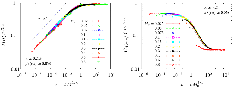
FIG. 5.: Scaling of the magnetization (left) and of the connected correlation function (right) for different initial conditions with magnetizations $M_{0}$.

We now present the numerical results obtained using the method described in the previous subsection. We first consider the scaling behavior of the magnetization and of the correlation as functions of the initial magnetization $M_{0}$. According to the theoretical prediction Eq. (30), we expect the magnetization to scale as

$$M(t,M_{0})=t^{-\frac{\beta}{\nu z}}\widehat{F}_{M}(tM_{0}^{1/\kappa})=t^{-0.057}\widehat{F}_{M}(tM_{0}^{4.02})\,,$$ (105)

where we have used the value of the critical exponent for the two-dimensional Ising model: $\beta=1/8$, $\nu=1$, $z=2.1667(5)$, and $\theta=0.383(3)$ (see,e.g., Ref. [2]), leading to $\kappa\simeq 0.249$ [see after Eq. (30)] and $\beta/(\nu z)\simeq 0.058$. For the short-time behavior one expects $\widehat{F}_{M}(x\rightarrow 0)\sim x^{\kappa}=x^{0.249}$. This scaling is rather well displayed by our data, as shown in Fig. 5.

Having tested the initial increase of the magnetization, we now consider the connected correlation function. In the previous sections we focussed on the scaling properties of the correlation for vanishing momentum $C_{{\bf q}=0}(t,s)$, whereas now we are interested in the behavior of the (auto)correlation function $C_{A}(t,s)=\int({\rm d}q)C_{\bf q}(t,s)$. According to the discussion in Sec. III, the scaling form of $C_{\bf q}(t,s)$ is given by Eq. (33) where the scaling function has an additional dependence on the variable $y\sim q^{z}(t-s)$. Accordingly we expect

$$C_{A}(t,s)=s(s/t)^{\frac{\beta\delta}{\nu z}}(t-s)^{a-\frac{d}{z}}\widehat{F}_{C}(s/t,M_{0}t^{\kappa})\,,$$ (106)

where the change $a\mapsto a-d/z$ is due to the integration over the momenta. To make evident the scaling with respect to $M_{0}$, we consider the correlation $C_{A}(t,t/3)$ for different initial magnetizations $M_{0}$. Thus we expect a data collapse for $t$ large enough according to

$$C_{A}(t,t/3)=t^{-2\frac{\beta}{\nu z}}\widehat{G}_{C}(tM_{0}^{\kappa})=t^{-0.11}\widehat{G}_{C}(tM_{0}^{4.02}).$$ (107)

where we used the relation $1+a-d/z=-2\beta/(\nu z)$. The corresponding data are reported in Fig. 5. Apart from a transient short-$t$ effect, we observe, again, a rather good data collapse.

C Correlations, Responses and $X^{\infty}$

We now specialize to completely ordered initial condition ($M_{0}=1$). According to Eqs. (34) and (35), the two-time connected correlation function and the integrated response TRM are expected to share the same critical scaling form which we write as

$$s^{2\beta/\nu z}C_{A}(t,s)=\widehat{f}_{C}(t/s)\,,\qquad{\rm and}\qquad s^{2\beta/\nu z}\rho(t,s)=\widehat{f}_{\rho}(t/s)\,,$$ (108)

with $2\beta/\nu z\approx 0.116$ and $f_{C,\rho}(x\gg 1)\sim x^{-\phi}$ where $\phi=-a+\frac{d}{z}+\frac{\beta\delta}{\nu z}=1+\beta(\delta+2)/(\nu z)\simeq 1.98$ (in two dimensions $\delta=15$). This behavior is again rather clearly displayed by our data, as Fig. 6 shows. Note however that due to the fast decay of the correlations, it is difficult to obtain good data for $x=t/s\gtrsim 20$ and that the TRM is affected by systematic deviations for the longer times.

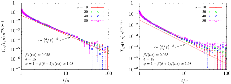
FIG. 6.: Scaling of the connected two-times correlation (left) and integrated response (right) functions for completely ordered initial conditions using Eq. (108).

Finally, we consider the value of the FDR that can be alternatively read off from the limit

$$X^{\infty}=\lim_{C_{A}\rightarrow 0}\frac{T_{c}\rho(t,s)}{C_{A}(t,s)}\,,$$ (109)

which indeed provides the estimate for $X^{\infty}$ as defined in Eq. (3). The plot in Fig. 7 clearly shows that $T_{c}\rho(t,s)/C_{A}(t,s)$ in Fig. 7 is rather well approximated by a straight line in a wide range of $x=s/t$, both in the case $M_{0}=0$ and $M_{0}\neq 0$. (This point was already observed in Ref. [36], see also [53]) The cross-over towards the quasi-equilibrium value $T_{c}\rho(t,s)/C_{A}(t,s)=1$ takes place for $x\sim 0.75$–$0.85$ (although the crossover is not complete in the set of data for the case $M_{0}=0$). A similar qualitative behavior is displayed by the field-theoretical Gaussian approximation for the same quantity, reported in Fig. 2. A more quantitative comparison, however, would require the analysis of the effects of fluctuations. In order to provide the numerical estimate for $X^{\infty}$ we use only the set of data which gives reasonable errors bars (typically $t/s\lesssim 20$), reported in Fig. 7. From these data, we roughly estimate

$$X^{\infty}_{\rm MC}=0.73(1)\,,$$ (110)

which compares rather well with the one-loop prediction $X^{\infty}\simeq 0.75$. Using the expression for $X^{\infty}$ provided in Ref. [30] (see also Subsec. V D) as an improved Gaussian approximation one gets $X^{\infty}=[3+2\beta/(\nu z)]/[4+2\beta/(\nu z)]\simeq 0.757$ which is indeed rather close to the numerical result.

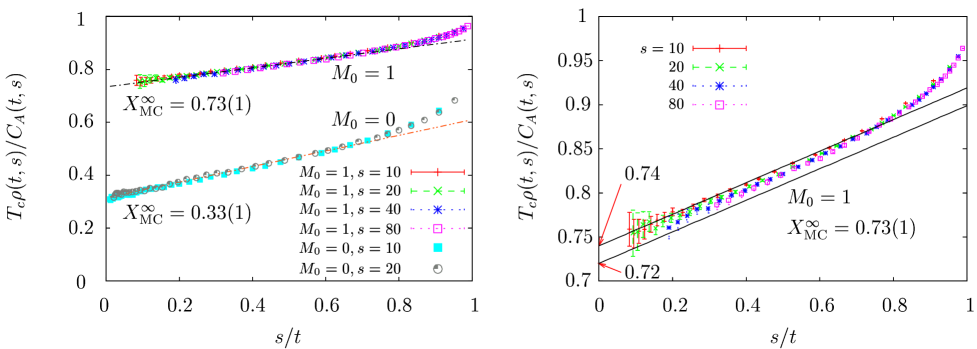
FIG. 7.: $T_{c}{\rho(t,s)}/{C_{A}(t,s)}$ versus $s/t$ for disorder and non disorder initial conditions (left). From our data we estimate $X^{\infty}_{\rm MC}=0.73(1)$ for ordered initial conditions (right).

VII Conclusions

In this paper we have considered the non-equilibrium dynamics of a system in the Ising universality class starting from a state with initial magnetization $M_{0}$ and evolving at criticality according to a purely dissipative dynamics. By means of RG arguments we found that in the aging regime ($t\gg s\gg\tau_{m}\sim M_{0}^{-1/\kappa}$) the zero-momentum response and connected correlation functions display the scaling behavior

$$R_{{\bf q}=0}(t,s) = \bar{A}_{R}\,(t-s)^{a}(t/s)^{\overline{\theta}}\bar{\mathcal{F}}_{R}(s/t)\;,$$ (111)

$$C_{{\bf q}=0}(t,s) = \bar{A}_{C}\,s(t-s)^{a}(t/s)^{{\overline{\theta}}^{\prime}}\bar{\mathcal{F}}_{C}(s/t)\;,$$ (112)

independently of the actual value of $M_{0}\neq 0$. We showed that the exponents ${\overline{\theta}}$ and ${\overline{\theta}}^{\prime}$ are not new non-equilibrium quantities, but they are given by standard equilibrium exponents as

$${\overline{\theta}}={\overline{\theta}}^{\prime}=-\frac{\beta\delta}{\nu z}\,.$$ (113)

In addition we showed that the ratio of the non-universal constants $\bar{A}_{R}$ and $\bar{A}_{C}$ with the corresponding ones obtained in the case $M_{0}=0$ are universal.

We solved exactly the dynamics within the Gaussian approximation and we derived all the relevant universal ratios and scaling functions. Then we considered the effect of fluctuations in order to provide more accurate predictions in physical dimensions $d=2,3$. We computed the first order correction in $\epsilon$-expansion to the response and to the connected correlation functions and from them we obtained the universal ratios and associated scaling functions. In particular, for the FDR we found

$$X^{\infty}=\frac{4}{5}-\left(\frac{73}{600}-\frac{\pi^{2}}{100}\right)\epsilon+O(\epsilon^{2})\,,$$ (114)

that gives $X^{\infty}\simeq 0.78$ in $d=3$ and $X^{\infty}\simeq 0.75$ in $d=2$. On the other hand, if the FDR is defined from the non-connected correlation function then the asymptotic value would be zero because of the scaling in the volume and times of the additional term $M(t)M(s)$.

In order to confirm our theoretical predictions we carried out extensive Monte Carlo simulation for the two-dimensional Ising model with Glauber dynamics using the approach of Refs. [43, 44]. We checked the predicted scaling forms for the two-time response and correlation functions in addition to the well-known scaling behavior of the magnetization [16]. Our analysis leads to a quite accurate determination of the FDR

$$X^{\infty}_{\rm MC}=0.73(1)\,,$$ (115)

which is in rather good agreement with the field-theoretical estimate.

It is worth noticing that at criticality $X^{\infty}<1$ independently of the initial magnetization. Therefore, insisting on the definition of an effective temperature, one finds $T_{\rm eff}\equiv T_{c}/X^{\infty}>T_{c}$. This fact can be naively understood for the case of a quench from high temperature to the critical point: The system, because of its slow dynamics, is somehow unable to transfer properly heat to the thermal bath, resulting in an effective higher value of the temperature. In the case of a sudden heating from a low-temperature configuration (with non-vanishing $M_{0}$ and given initial short-range correlations $\Delta_{0}$) to the critical point one would have expected (as observed in some cases [52]) $T_{\rm eff}$ being larger than the initial temperature but smaller than $T_{c}$. This is not the case here, showing that the properties of $T_{{\rm eff}}$ at criticality are both non trivial and counter-intuitive.

Let us now compare our results with those available in the literature. To our knowledge the ageing properties of the non-equilibrium critical relaxation from an ordered (alternatively magnetized) state has been the subject of three recent studies [31, 30, 9]. In Ref. [30] the lattice Ising model with Glauber dynamics has been solved in the mean-field cases of (a) fully connected lattice (infinite interaction range) and (b) nearest-neighbor interaction in the limit of large dimensionality $d$. The corresponding results are completely equivalent to our Gaussian solution, as expected. In Ref. [9] the ageing properties of the spherical model with relaxational dynamics have been considered. The scaling forms for response and correlation functions found there agree with our general predictions. In this case $X^{\infty}$ is a monotonic function of the dimensionality $d$, interpolating between $1/2$ at $d=2$ and $4/5$ at $d=4$. This shares with our result for $d<4$ a downward correction to the Gaussian result $4/5$. However a more quantitative comparison is clearly not possible, since the two models belong to different universality classes. The non-linear $\sigma$-model has been used to study the critical aging dynamics of ferromagnetic systems with $O(N)$ symmetry ($N>2$) in Ref. [31]. Correlation and response functions are computed in a dimensional $\tilde{\epsilon}$-expansion around the lower critical dimension $d=2$, with $\tilde{\epsilon}=d-2$, leading to $X^{\infty}=1/2+O(\tilde{\epsilon})$. These results do not compare directly with ours, since the behavior of $O(N)$ models is affected by the massless fluctuation modes in the directions transverse to the decaying magnetization, in addition to the longitudinal one. In order to make a contact with Refs. [31, 9] we have also studied the non-equilibrium aging dynamics of the $O(N)$ model up to first-order in the $\epsilon$-expansion. The analysis will appear elsewhere [54].

A Feynman diagrams for the response function

There are two one-particle irreducible (1PI, i.e., that cannot be disconnected by cutting one propagator) diagrams entering in the calculation of the response function [see Fig. 3]. One is $I(t)$ [see Eq. (79), depicted in Fig. 3(1)] and the other is the “bubble” in Fig. 3(2):

$$B_{RC}(t_{1},s_{1})=\int({\rm d}q)R^{0}_{\bf q}(t_{1},s_{1})C^{0}_{\bf q}(t_{1},s_{1})\,.$$ (A1)

For $t_{1}>s_{1}$ [because of causality, $B_{RC}(t_{1}\leq s_{1},s_{1})=0$]

$$B_{RC}(t_{1},s_{1}) = \int({\rm d}q)\left(\frac{s_{1}}{t_{1}}\right)^{3/2}{\rm e}^{-{\bf q}^{2}(t_{1}-s_{1})}\frac{2}{(t_{1}s_{1})^{3/2}}{\rm e}^{-{\bf q}^{2}(t_{1}+s_{1})}\int_{0}^{s_{1}}{\rm d}xx^{3}{\rm e}^{2{\bf q}^{2}x}$$ (A2)

$$= 2(8\pi)^{-\frac{d}{2}}H_{d}(t_{1},s_{1})$$ (A3)

with

$$H_{d}(t_{1},s_{1}) = t_{1}^{-3}\int_{0}^{s_{1}}{\rm d}x\;x^{3}(t_{1}-x)^{-\frac{d}{2}}$$ (A4)

$$= A_{d}t_{1}^{-1+\epsilon/2}-A_{d}t_{1}^{-1}(t_{1}-s_{1})^{\epsilon/2}+B_{d}t_{1}^{-2}s_{1}(t_{1}-s_{1})^{\epsilon/2}+C_{d}t_{1}^{-3}s_{1}^{2}(t_{1}-s_{1})^{\epsilon/2}$$ (A6)

$$+D_{d}t_{1}^{-3}s_{1}^{3}(t_{1}-s_{1})^{-1+\epsilon/2}\,,$$

where

$$A_{d} = \frac{6}{(2+\epsilon/2)(1+\epsilon/2)\epsilon/2(-1+\epsilon/2)}\,,$$ (A7)

$$B_{d} = -\frac{6}{(2+\epsilon/2)(1+\epsilon/2)(-1+\epsilon/2)}\,,$$ (A8)

$$C_{d} = -\frac{3}{(2+\epsilon/2)(-1+\epsilon/2)}\,,$$ (A9)

$$D_{d} = -\frac{1}{(-1+\epsilon/2)}\,.$$ (A10)

This parameterization is convenient because all the divergences arises only from those terms containing $A_{d}$ or $D_{d}$.

Thus the integrals for the response function read (as usual $x=s/t$)

$$I_{1}(t,s) = \int_{s}^{t}{\rm d}t^{\prime}R^{0}_{{\bf q}=0}(t,t^{\prime})I(t^{\prime})R^{0}_{{\bf q}=0}(t^{\prime},s)=\int_{s}^{t}{\rm d}t^{\prime}(t^{\prime}/t)^{3/2}(s/t^{\prime})^{3/2}2N_{d}r_{d}t^{\prime 1-d/2}$$ (A11)

$$= 2N_{d}r_{d}(s/t)^{3/2}\frac{t^{2-d/2}-s^{2-d/2}}{2-d/2}=2N_{d}r_{d}(s/t)^{3/2}s^{\epsilon/2}\left[-\ln x+\frac{1}{4}\epsilon\ln^{2}x+O(\epsilon^{2})\right],$$ (A12)

corresponding to Fig. 3(1) and

$$I_{2}(t,s) = \int_{s}^{t}{\rm d}t_{1}\int_{s}^{t_{1}}{\rm d}s_{1}R^{0}_{{\bf q}=0}(t,t_{1})\sqrt{2}m_{G}(t_{1})B(t_{1},s_{1})\sqrt{2}m_{G}(s_{1})R^{0}_{{\bf q}=0}(s_{1},s)$$ (A13)

$$= 6(8\pi)^{-\frac{d}{2}}\left(\frac{s}{t}\right)^{3/2}\int_{s}^{t}{\rm d}t_{1}\,t_{1}\int_{s}^{t_{1}}{\rm d}s_{1}\,s_{1}^{-2}H_{d}(t_{1},s_{1})\,$$ (A14)

corresponding to Fig. 3(2). Using the parameterization (A6) for $H_{d}$, $I_{2}$ is reduced to five simple integrals whose sum is

$$I_{2}(t,s)=\frac{6s^{\epsilon/2}}{(8\pi)^{d/2}}\left(\frac{s}{t}\right)^{3/2} \left[-\frac{2}{\epsilon}\ln x-\frac{1-x}{2}+\frac{\pi^{2}}{3}+3\ln(1-x)\left(\frac{1}{x}-1\right)+\frac{3}{2}\ln x\right.$$ (A16)

$$\left.+\frac{1}{2}\ln^{2}x-2{\rm Li}_{2}(x)+O(\epsilon)\right]\,,$$

with $x=s/t$ and ${\rm Li}_{2}(x)\equiv\sum_{n=1}^{\infty}x^{n}/n^{2}$.

B Feynman diagrams for the correlation function

There is only one new 1PI diagram for the correlation functions, depicted in Fig. 4(5) [we define $t_{<}=\min\{t,t^{\prime}\}$]:

$$B_{CC}(t,t^{\prime}) = \int({\rm d}q)[C^{0}_{\bf q}(t,t^{\prime})]^{2}=\int({\rm d}q)4(tt^{\prime})^{-3}{\rm e}^{-2{\bf q}^{2}(t+t^{\prime})}\int_{0}^{t_{<}}{\rm d}t_{1}t_{1}^{3}{\rm e}^{2{\bf q}^{2}t_{1}}\int_{0}^{t_{<}}{\rm d}t_{2}t_{2}^{3}{\rm e}^{2{\bf q}^{2}t_{2}}=$$ (B1)

$$= \frac{4(tt^{\prime})^{-3}}{(8\pi)^{d/2}}\int_{0}^{t_{<}}{\rm d}t_{1}\int_{0}^{t_{<}}{\rm d}t_{2}\frac{t_{1}^{3}t_{2}^{3}}{(t+t^{\prime}-t_{1}-t_{2})^{d/2}}\,.$$ (B2)

This enter in the connected diagram represented in Fig. 4(5) [we assume $t>s$, given that $I_{5}(t,s)=I_{5}(s,t)$]:

$$I_{5}(t,s) = \int_{0}^{s}{\rm d}\tau_{1}\int_{0}^{t}{\rm d}\tau_{2}\,R^{0}_{{\bf q}=0}(s,\tau_{1})\sqrt{2}m_{G}(\tau_{1})B_{CC}(\tau_{1},\tau_{2})\sqrt{2}m_{G}(\tau_{2})R^{0}_{{\bf q}=0}(t,\tau_{2})$$ (B3)

$$= \int_{0}^{s}{\rm d}\tau_{1}\int_{0}^{s}{\rm d}\tau_{2}(s/\tau_{1})^{-3/2}(3/\tau_{1})^{1/2}B_{CC}(\tau_{1},\tau_{2})(3/\tau_{2})^{1/2}(t/\tau_{2})^{-3/2}$$ (B5)

$$+\int_{0}^{s}{\rm d}\tau_{1}\int_{s}^{t}{\rm d}\tau_{2}(s/\tau_{1})^{-3/2}(3/\tau_{1})^{1/2}B_{CC}(\tau_{1},\tau_{2})(3/\tau_{2})^{1/2}(t/\tau_{2})^{-3/2}$$

$$= 3(st)^{-3/2}\left[2\int_{0}^{s}{\rm d}\tau_{1}\int_{0}^{\tau_{1}}{\rm d}\tau_{2}\,\tau_{1}\tau_{2}B_{CC}(\tau_{1},\tau_{2})+\int_{0}^{s}{\rm d}\tau_{1}\int_{s}^{t}{\rm d}\tau_{2}\,\tau_{1}\tau_{2}B_{CC}(\tau_{1},\tau_{2})\right]$$ (B6)

$$= 3(st)^{-3/2}[2B+A]\,.$$ (B7)

It is easy to realize that both $A$ and $B$ do not diverge for $d\to 4$. Therefore no dimensional regularization is required and one can calculate them directly in $d=4$:

$$A = 4(8\pi)^{-\frac{d}{2}}\int_{0}^{s}{\rm d}\tau_{1}\int_{s}^{t}{\rm d}\tau_{2}\frac{1}{(\tau_{1}\tau_{2})^{2}}\int_{0}^{\tau_{1}}{\rm d}t_{1}\int_{0}^{\tau_{1}}{\rm d}t_{2}\frac{t_{1}^{3}t_{2}^{3}}{(\tau_{1}+\tau_{2}-t_{1}-t_{2})^{2}}+O(\epsilon)$$ (B8)

$$= 4(8\pi)^{-\frac{d}{2}}s^{4}\left[{\cal A}(s/t)-\frac{81}{200}-\frac{\pi^{2}}{40}+\frac{24}{25}\ln 2\right]+O(\epsilon)\,,$$ (B9)

$$B = 4(8\pi)^{-\frac{d}{2}}\int_{0}^{s}{\rm d}\tau_{1}\int_{0}^{\tau_{1}}{\rm d}\tau_{2}\frac{1}{(\tau_{1}\tau_{2})^{2}}\int_{0}^{\tau_{2}}{\rm d}t_{1}\int_{0}^{\tau_{2}}{\rm d}t_{2}\frac{t_{1}^{3}t_{2}^{3}}{(\tau_{1}+\tau_{2}-t_{1}-t_{2})^{2}}+O(\epsilon)$$ (B10)

$$= 4(8\pi)^{-\frac{d}{2}}s^{4}\left(\frac{1447}{4800}+\frac{\pi^{2}}{160}-\frac{12}{25}\ln 2\right)+O(\epsilon)\;,$$ (B11)

where

$${\cal A}(x)=\frac{1}{4}\int_{0}^{x}{\rm d}y_{1}\,(y_{1}^{4}x^{-4}-1)\int_{0}^{1}{\rm d}x_{1}\int_{0}^{1}{\rm d}x_{2}\frac{x_{1}^{3}x_{2}^{3}}{(1+y_{1}^{-1}-x_{1}-x_{2})^{2}}\,,$$ (B12)

is a negative and monotonically decreasing function with ${\cal A}(x)=-x^{3}/252+O(x^{4})$ and ${\cal A}(1)=\frac{1153}{3600}+\frac{\pi^{2}}{30}-\frac{24}{25}\ln 2\simeq-0.016$. [Although ${\cal A}(x)$ can be expressed in terms of elementary functions we do not report here its lengthy form.] Thus

$$I_{5}(t,s)=3(st)^{-3/2}[A+2B]=\frac{s(s/t)^{3/2}}{(8\pi)^{d/2}}\left[\left(\frac{19}{8}-\frac{3\pi^{2}}{20}\right)+12{\cal A}(s/t)\right]+O(\epsilon)\,.$$ (B13)

There are two diagrams involving $B_{RC}(t_{1},s_{1})$ [see Fig. 4(6)], namely

$$I_{6}(t,s) = \int_{0}^{t}{\rm d}t_{2}\int_{t_{2}}^{t}{\rm d}t_{1}\,R^{0}_{{\bf q}=0}(t,t_{1})\sqrt{2}m_{G}(t_{1})B_{RC}(t_{1},t_{2})\sqrt{2}m_{G}(t_{2})C^{0}_{{\bf q}=0}(t_{2},s)+$$ (B15)

$$\int_{0}^{s}{\rm d}t_{1}\int_{t_{1}}^{s}{\rm d}t_{2}\,C^{0}_{{\bf q}=0}(t,t_{1})\sqrt{2}m_{G}(t_{1})B_{RC}(t_{2},t_{1})\sqrt{2}m_{G}(t_{2})R^{0}_{{\bf q}=0}(s,t_{2})\,,$$

that can be written as

$$I_{6}(t,s) =\frac{3}{2}(st)^{-3/2} \left[\int_{0}^{s}{\rm d}t_{2}\,t_{2}^{2}\int_{t_{2}}^{t}{\rm d}\,t_{1}t_{1}B_{RC}(t_{1},t_{2})+s^{4}\int_{s}^{t}{\rm d}t_{2}\,t_{2}^{-2}\int_{t_{2}}^{t}{\rm d}t_{1}\,t_{1}B_{RC}(t_{1},t_{2})\right.$$ (B17)

$$\left.+\int_{0}^{s}{\rm d}t_{1}\,t_{1}^{2}\int_{t_{1}}^{s}{\rm d}t_{2}\,t_{2}B_{RC}(t_{2},t_{1})\right]\,.$$

Using the parameterization of Eq. (A6), each of the three integrals decomposes in five integrals that can be easily computed. Therefore

$$I_{6}(t,s)=\frac{3}{2}(st)^{-3/2}[(A)+(B)+(C)]=\frac{3(st)^{-3/2}}{(8\pi)^{\frac{d}{2}}}\sum_{a\in{A,B,C}}\sum_{i=1}^{5}(a)_{i}$$ (B18)

where

$$(A)_{1} = \frac{A_{d}}{1+\epsilon/2}\left[\frac{t^{1+\epsilon/2}s^{3}}{3}-\frac{s^{4+\epsilon/2}}{4+\epsilon/2}\right]$$ (B19)

$$(A)_{2} = -\frac{A_{d}}{1+\epsilon/2}\left[\frac{s^{3}t}{3}-\frac{s^{4}}{4}+\frac{\epsilon}{2}\left(s\frac{9s^{3}-4s^{2}t-6st^{2}-12t^{3}}{144}\right.\right.$$ (B21)

$$\left.\left.+\frac{t^{4}}{12}\ln t-\frac{3s^{4}-4s^{3}t+t^{4}}{12}\ln(t-s)\right)+O(\epsilon^{2})\right]$$

$$(A)_{3} = \frac{B_{d}s^{4}}{4}\left[\frac{1}{4}+\ln\frac{t}{s}\right]+O(\epsilon)$$ (B22)

$$(A)_{4} = C_{d}\left[\frac{s^{4}}{4}-\frac{s^{5}}{5t}\right]+O(\epsilon)$$ (B23)

$$(A)_{5} = D_{d}\left[\frac{s^{4}}{2\epsilon}-\frac{3}{8}s^{4}+\frac{s^{5}}{5t}-\frac{s^{3}t}{12}-\frac{s^{2}t^{2}}{8}-\frac{st^{3}}{4}-\frac{s^{4}}{4}\ln\frac{t}{s}+\frac{s^{4}-t^{4}}{4}\ln(t-s)+\frac{t^{4}}{4}\ln t\right]+O(\epsilon)$$ (B24)

$$(B)_{1} = \frac{s^{4}A_{d}}{1+\epsilon/2}\left[t^{\epsilon/2}\left(\frac{t}{s}-1\right)-\frac{2}{\epsilon}\left(t^{\epsilon/2}-s^{\epsilon/2}\right)\right]$$ (B25)

$$(B)_{2} = -\frac{s^{4}A_{d}}{1+\epsilon/2}\left[\frac{t}{s}-1-\ln\frac{t}{s}+\frac{\epsilon}{2}\left(\frac{\pi^{2}}{6}+\ln t\ln s-\ln^{2}t-\ln\frac{t}{s}+\left(\frac{t}{s}-1\right)\ln(t-s)-{\rm Li}_{2}\frac{s}{t}\right)\right]$$ (B27)

$$+O(\epsilon)$$

$$(B)_{3} = \frac{s^{4}B_{d}}{2}\ln^{2}\frac{t}{s}$$ (B28)

$$(B)_{4} = C_{d}s^{4}\left(\ln\frac{t}{s}-\frac{t-s}{t}\right)$$ (B29)

$$(B)_{5} = D_{d}s^{4}\left[\frac{2}{\epsilon}\ln\frac{t}{s}-\ln\frac{t}{s}+\frac{t-s}{t}-\frac{1}{2}\ln^{2}\frac{t}{s}+\ln^{2}t-\frac{\pi^{2}}{6}-\ln t\ln s+{\rm Li}_{2}\frac{s}{t}\right]+O(\epsilon)$$ (B30)

$$(C)_{1} = \frac{A_{d}}{1+\epsilon/2}s^{4+\epsilon/2}\left(\frac{1}{3}-\frac{1}{4+\epsilon/2}\right)$$ (B31)

$$(C)_{2} = -\frac{A_{d}}{1+\epsilon/2}\frac{2s^{4+\epsilon/2}}{(2+\epsilon/2)(3+\epsilon/2)(4+\epsilon/2)}$$ (B32)

$$(C)_{3} = \frac{B_{d}}{16}s^{4}+O(\epsilon)$$ (B33)

$$(C)_{4} = \frac{C_{d}}{20}s^{4}+O(\epsilon)$$ (B34)

$$(C)_{5} = D_{d}s^{4}\left[\frac{1}{2\epsilon}-\frac{19}{30}+\frac{1}{4}\ln s\right]+O(\epsilon)$$ (B35)

Summing up one finds

$$I_{6}(t,s) = \frac{3s^{4}(st)^{-3/2}}{(8\pi)^{d/2}}\left[\frac{1-2\ln x}{\epsilon}+\frac{\pi^{2}}{3}-\frac{271}{60}\right.$$ (B37)

$$+\left.2\ln x+\ln t\left(\frac{1}{2}-\ln x\right)-\frac{\ln^{2}x}{2}+{\cal B}(x)\right]+O(\epsilon)\,.$$

where

$${\cal B}(x)=\frac{2x}{5}-\frac{7}{2}\ln(1-x)-2\text{Li}_{2}(x)+\frac{31}{8}+\frac{4\ln(1-x)}{x}-\frac{1}{2x^{4}}\left[\ln(1-x)+x+\frac{x^{2}}{2}+\frac{x^{3}}{3}\right]$$ (B38)

is a monotonically increasing function with ${\cal B}(x)=x^{3}/63+O(x^{4})$ and ${\cal B}(1)=\frac{403}{120}-\frac{\pi^{2}}{3}\simeq 0.068$.

The diagram involving $I(t)$ is [see Fig. 4(7)]

$$I_{7}(t,s) = \int_{0}^{s}{\rm d}t^{\prime}\,R^{0}_{{\bf q}=0}(t^{\prime},s)I(t^{\prime})C^{0}_{{\bf q}=0}(t,t^{\prime})+\int_{0}^{t}{\rm d}t^{\prime}\,R^{0}_{{\bf q}=0}(t^{\prime},t)I(t^{\prime})C^{0}_{{\bf q}=0}(t^{\prime},s)=$$ (B39)

$$= N_{d}r_{d}\left[2(st)^{-3/2}\int_{0}^{s}{\rm d}t^{\prime}\,t^{\prime 5-d/2}+\frac{s^{5/2}}{t^{3/2}}\int_{s}^{t}{\rm d}t^{\prime}\,t^{\prime 1-d/2}\right]=$$ (B40)

$$= N_{d}r_{d}s\left(\frac{s}{t}\right)^{3/2}s^{\epsilon/2}\left\{\frac{2}{4+\epsilon/2}+\frac{2}{\epsilon}\left[\left(\frac{t}{s}\right)^{\epsilon/2}-1\right]\right\}\,.$$ (B41)

Finally there is the contribution coming from the one-loop correction to the magnetization. At this order in perturbation theory it can be simply evaluated as

$$C_{{\bf q}=0}^{0}(t,s)=2\int_{0}^{s}{\rm d}t_{2}\,\exp\left[-\left(2\int_{t_{2}}^{s}{\rm d}t_{1}\,m^{2}(t_{1})+\int_{s}^{t}{\rm d}t_{1}\,m^{2}(t_{1})\right)\right]\,.$$ (B42)

Using the value of $m^{2}(t)$ given by Eq. (82), we obtain

$$C_{{\bf q}=0}^{0}(t,s) = 2\int_{0}^{s}{\rm d}t_{2}\,\exp\left\{-3\int_{t_{2}}^{s}\frac{{\rm d}t_{1}}{t_{1}}\left(1-2\tilde{g}\frac{r_{d}}{1+\epsilon/2}t_{1}^{\epsilon/2}\right)-\frac{3}{2}\int_{s}^{t}\frac{{\rm d}t_{1}}{t_{1}}\left(1-2\tilde{g}\frac{r_{d}}{1+\epsilon/2}t_{1}^{\epsilon/2}\right)\right\}=$$ (B43)

$$= 2\int_{0}^{s}{\rm d}t_{2}\left(\frac{t_{2}}{s}\right)^{3}\left(\frac{s}{t}\right)^{3/2}\left\{1+\frac{6\tilde{g}r_{d}}{1+\epsilon/2}\left[\frac{2}{\epsilon}(s^{\epsilon/2}-t_{2}^{\epsilon/2})+\frac{1}{\epsilon}\left(t^{\epsilon/2}-s^{\epsilon/2}\right)\right]+O(\tilde{g}^{2})\right\}=$$ (B44)

$$= \frac{1}{2}s\left(\frac{s}{t}\right)^{3/2}\left\{1+\frac{6\tilde{g}r_{d}s^{\epsilon/2}}{1+\epsilon/2}\left[\frac{1}{4+\epsilon/2}+\frac{1}{\epsilon}\left(\left(\frac{t}{s}\right)^{\epsilon/2}-1\right)\right]\right\}\,.$$ (B45)

Summing up all the contributions according to Eq. (94) one finds

$$C_{{\bf q}=0}(t,s)=\frac{1}{2}s\left(\frac{s}{t}\right)^{3/2}\left[1+\tilde{g}\left(-\frac{719}{320}+\frac{37}{160}\pi^{2}-\frac{3}{8}\ln x\right)+\tilde{g}f_{C}(s/t)+O(\tilde{g}^{2},\epsilon\tilde{g})\right]\,,$$ (B46)

with

$$f_{C}(x) = \frac{3x}{10}+12{\cal A}(x)+3{\cal B}(x)-\frac{21}{8}\ln(1-x)-\frac{3{\rm Li}_{2}(x)}{2}+\frac{93}{32}+$$ (B48)

$$+\frac{3\ln(1-x)}{x}-\frac{3}{8x^{4}}\left[\ln(1-x)+x+\frac{x^{2}}{2}+\frac{x^{3}}{3}\right]\,,$$

[$f_{C}(0)=0$] where ${\cal A}(x)$ and ${\cal B}(x)$ are given by Eqs. (B12) and (B38).

REFERENCES

• [1] E. Vincent, J. Hammann, M. Ocio, J. P. Bouchaud, and L. F. Cugliandolo, Slow dynamics and aging in spin-glasses, 1997 Lect. Notes Phys. 492 184 [cond-mat/9607224];
Bouchaud J P, Cugliandolo L F, Kurchan J and Mézard M Out of equilibrium dynamics in spin-glasses and other glassy systems, 1998 in Spin Glasses and Random Fields, Directions in Condensed Matter Physics, vol 12 ed A P Young (Singapore: World Scientific) [cond-mat/9702070];
L. F. Cugliandolo, Dynamics of glassy systems, Lecture notes, Les Houches, July 2002 [cond-mat/0210312];
A. Crisanti and F. Ritort, Violation of the fluctuation-dissipation theorem in glassy systems: basic notions and the numerical evidence, 2003 J. Phys. A 36 R181 [cond-mat/0212490].
• [2] P. Calabrese and A. Gambassi, Aging Properties of Critical Systems: A Field-Theoretical Approach, 2005 J. Phys. A 38 R133 [cond-mat/0410357]
• [3] A. Gambassi, Slow dynamics at critical points: the field-theoretical perspective, 2005 Proc. of the Int. Summer School “Ageing and the Glass Transition” to appear in J. Phys.: Conf. Series.
• [4] L. F. Cugliandolo and J. Kurchan, Analytical Solution of the Off-Equilibrium Dynamics of a Long Range Spin-Glass Model, 1993 Phys. Rev. Lett. 71 173 [cond-mat/9303036]; On the Out of Equilibrium Relaxation of the Sherrington - Kirkpatrick model, 1994 J. Phys. A 27 5749 [cond-mat/9311016]; Weak-ergodicity breaking in mean-field spin-glass models, 1995 Phil. Mag. B 71 50 [cond-mat/9403040].
• [5] L. F. Cugliandolo, J. Kurchan, and G. Parisi, Off equilibrium dynamics and aging in unfrustrated systems, 1994 J. Phys. I (France) 4 1641 [cond-mat/9406053].
• [6] L. F. Cugliandolo, J. Kurchan, and L. Peliti, Energy flow, partial equilibration and effective temperatures in systems with slow dynamics, 1997 Phys. Rev. E 55 3898 [cond-mat/9611044].
• [7] P. Calabrese and A. Gambassi, Aging in ferromagnetic systems at criticality near four dimensions, 2002 Phys Rev. E 65 066120 [cond-mat/0203096]; 2002 Acta Phys. Slov. 52 311.
• [8] G. Schehr and R. Paul, Universal aging properties at a disordered critical point, 2005 Phys. Rev. E 72 016105 [cond-mat/0412447].
• [9] A. Annibale and P. Sollich, Spin, bond and global fluctuation-dissipation relations in the non-equilibrium spherical ferromagnet, 2006 J. Phys. A 39 2853 [cond-mat/0510731].
• [10] P. Calabrese and A. Gambassi, On the definition of a unique effective temperature for non-equilibrium critical systems, 2004 J. Stat. Mech.: Theor. Exp. P07013 [cond-mat/0406289]
• [11] P. C. Hohenberg and B. I. Halperin, Theory of dynamic critical phenomena, 1977 Rev. Mod. Phys. 49 435.
• [12] Z. Rácz, Nonlinear relaxation near the critical point: molecular-field and scaling theory, 1976 Phys. Rev. B 13 263
• [13] M. E. Fisher and Z. Racz, Scaling theory of nonlinear relaxation, 1976 Phys. Rev. B 13 5039
• [14] R. Bausch and H. K. Janssen, Equation of Motion and Nonlinear Response near the Critical point, 1976 Z. Phys. B 25 275
• [15] R. Bausch, E. Eisenriegler, and H. K. Janssen, Nonlinear Critical Slowing Down of the One-Component Ginzburg-Landau Field, 1979 Z. Phys. B 36 179
• [16] H. K. Janssen, B. Schaub, and B. Schmittmann, New universal short-time scaling behaviour of critical relaxation processes, 1989 Z. Phys B 73 539.
• [17] H. K. Janssen, On the renormalized field theory of nonlinear critical relaxation, in From Phase Transitions to Chaos– Topics in Modern Statistical Physics, edited by G. Györgyi, I. Kondor, L. Sasvári, T. Tel (World Scientific, Singapore, 1992).
• [18] C. Godrèche and J. M. Luck, Response of non-equilibrium systems at criticality: ferromagnetic models in dimension two and above, 2000 J. Phys. A 33 9141 [cond-mat/0001264]
• [19] C. Godrèche and J. M. Luck, Nonequilibrium critical dynamics of ferromagnetic spin systems, 2002 J. Phys.: Condens. Matter 14 1589 [cond-mat/0109212]
• [20] P. Calabrese and A. Gambassi, Two-loop Critical Fluctuation-Dissipation Ratio for the Relaxational Dynamics of the $O(N)$ Landau-Ginzburg Hamiltonian, 2002 Phys Rev. E 66 066101 [cond-mat/0207452].
• [21] P. Calabrese and A. Gambassi, Aging and fluctuation-dissipation ratio for the dilute Ising Model, 2002 Phys. Rev. B 66 212407 [cond-mat/0207487].
• [22] A. Picone and M. Henkel Response of non-equilibrium systems with long-range initial correlations, 2002 J. Phys. A 35 5575 [cond-mat/0203411]
• [23] P. Calabrese and A. Gambassi, Aging at Criticality in Model C Dynamics, 2003 Phys. Rev. E 67 036111 [cond-mat/0211062].
• [24] M. Henkel and G. M. Schütz, On the universality of the fluctuation-dissipation ratio in non-equilibrium critical dynamics, 2004 J. Phys. A 37 591 [cond-mat/0308466]
• [25] Y. Chen and Z.-B. Li, Short-time dynamics of spin systems with long-range correlated quenched impurities, 2005 Phys. Rev. B 71 174433
• [26] M. Pleimling, Aging phenomena in critical semi-infinite systems, 2004 Phys. Rev. B 70 104401 [cond-mat/0404203]
• [27] F. Baumann and M. Pleimling, Out-of-equilibrium properties of the semi-infinite kinetic spherical model, 2006 J. Phys. A 39 1981 [cond-mat/0509064]
• [28] U. Ritschel and H. W. Diehl, Dynamical relaxation and universal short-time behavior in finite systems, The renormalization-group approach, 1996 Nucl. Phys. B 464 512 [cond-mat/9510077]
• [29] Z.-B. Li, U. Ritschel, and B. Zheng, Monte Carlo simulation of universal short-time behavior in critical relaxation, 1994 J. Phys. A 27 L837 [cond-mat/9409058]; H. W. Diehl and U. Ritschel, Dynamical relaxation and universal short-time behavior of finite systems, 1993 J. Stat. Phys. 73 1; U. Ritschel and H. W. Diehl, Long-time traces of the initial condition in relaxation phenomena near criticality, 1995 Phys. Rev. E 51 5392 [cond-mat/9409057]
• [30] A. Garriga A, P. Sollich P, I. Pagonabarraga, and F. Ritort, Universality of Fluctuation-Dissipation Ratios: The Ferromagnetic Model, 2005 Phys. Rev. E 72 056114 [cond-mat/0508243].
• [31] A. A. Fedorenko and S. Trimper, Critical aging of a ferromagnetic system from a completely ordered state, 2006 Europhys. Lett. 74 89 [cond-mat/0507112].
• [32] R. J. Glauber, Time-Dependent Statistics of Ising Model, 1963 J. Math. Phys. 4 294.
• [33] E. Lippiello and M. Zannetti, Fluctuation dissipation ratio in the one dimensional kinetic Ising model, 2000 Phys. Rev. E 61 3369 [cond-mat/0001103].
• [34] C. Godrèche and J. M. Luck, Response of non-equilibrium systems at criticality: Exact results for the Glauber-Ising chain, 2000 J. Phys. A 33 1151 [cond-mat/9911348].
• [35] L. R. Fontes, M. Isopi, C. M. Newman, and D. L. Stein, Aging in 1D Discrete Spin Models and Equivalent Systems, 2001 Phys. Rev. Lett. 87 110201 [cond-mat/0103494].
• [36] P. Mayer, L. Berthier, J. P. Garrahan, and P. Sollich, Fluctuation-dissipation relations in the non-equilibrium critical dynamics of Ising models, 2003 Phys. Rev. E 68 016116 [cond-mat/0301493].
• [37] P. Mayer and P. Sollich, General Solutions for Multispin Two-Time Correlation and Response Functions in the Glauber-Ising Chain, 2004 J. Phys. A 37 9 [cond-mat/0307214].
• [38] J. Zinn-Justin, Quantum Field Theory and Critical Phenomena, 3rd edition (Clarendon, Oxford, 1996).
• [39] H. K. Janssen, On a Lagrangian for classical field dynamics and renormalization group calculations of dynamical critical properties, 1976 Z. Phys. B 23 377;
R. Bausch, H. K. Janssen, and H. Wagner, Renormalized field theory of critical dynamics, 1976 Z. Phys. B 24 113.
• [40] H. W. Diehl, The theory of boundary critical phenomena, in Phase Transitions and Critical Phenomena, edited by C. Domb and J. L. Lebowitz, Vol. 10 (Academic Press, London, 1986); H. W. Diehl, The Theory of Boundary Critical Phenomena 1997 Int. J. Mod. Phys. B 11 3503 [cond-mat/9610143]
• [41] L. F. Cugliandolo, D. S. Dean, and J. Kurchan, Fluctuation-Dissipation theorems and entropy production in relaxational systems, 1997 Phys. Rev. Lett. 79 2168 [cond-mat/9705002]
• [42] F. Sastre, I. Dornic, and H. Chaté, Nominal Thermodynamic Temperature in Nonequilibrium Kinetic Ising Models, 2003 Phys. Rev. Lett. 91 267205 [cond-mat/0308178].
• [43] C. Chatelain, A far-from-equilibrium fluctuation-dissipation relation for an Ising-Glauber-like model, 2003 J. Phys. A 36 10739 [cond-mat/0303545].
• [44] F. Ricci-Tersenghi, Measuring the fluctuation-dissipation ratio in glassy systems with no perturbing field, 2003 Phys. Rev. E 68 065104(R) [cond-mat/0307565].
• [45] C. Chatelain, On universality in aging ferromagnets, 2004 J. Stat. Mech.: Theor. Exp. P06006 [cond-mat/0404017].
• [46] S. Abriet and D. Karevski, Off equilibrium dynamics in 2d-XY system, 2004 Eur. Phys. J. B 37 47 [cond-mat/0309342]; Off equilibrium dynamics in the 3d-XY system, 2004 Eur. Phys. J. B 41 79 [cond-mat/0405598].
• [47] C. Godrèche, F. Krzakala and F. Ricci-Tersenghi, Nonequilibrium critical dynamics of the ferromagnetic Ising model with Kawasaki dynamics, 2004 J. Stat. Mech.: Theor. Exp. P04007 [cond-mat/0401334].
• [48] F. Krzakala, Glassy properties of the Kawasaki dynamics of two-dimensional ferromagnets, 2005 Phys. Rev. Lett. 94, 077204 [cond-mat/0409348].
• [49] A. Barrat, Monte-Carlo simulations of the violation of the fluctuation-dissipation theorem in domain growth processes, 1998 Phys. Rev. E 57 3629 [cond-mat/9710069].
• [50] F. Corberi, E. Lippiello E and M. Zannetti Effective temperature in the quench of coarsening systems to and below $T_{C}$, 2004 J. Stat. Mech.: Theor. Exp. P12007 [cond-mat/0412088]
• [51] M. Pleimling and A. Gambassi, Corrections to local scale invariance in the non-equilibrium dynamics of critical systems: numerical evidences, 2005 Phys. Rev. B 71 180401(R) [cond-mat/0501483]
• [52] F. Krzakala and F. Ricci-Tersenghi, Aging, memory and rejuvenation: some lessons from simple models, cond-mat/0512309.
• [53] M. Pleimling, Comment on ”Fluctuation-dissipation relations in the nonequilibrium critical dynamics of Ising models”, 2004 Phys. Rev. E 70 018101 [cond-mat/0309652];
P. Mayer, L. Berthier, J. P. Garrahan, and P. Sollich Reply to Comment on ”Fluctuation-dissipation relations in the non-equilibrium critical dynamics of Ising models”, 2004 Phys. Rev. E 70 018102 [cond-mat/0310545]
• [54] P. Calabrese and A. Gambassi, 2006 to appear.