Electronic states and Landau levels in graphene stacks

Abstract

We analyze, within a minimal model that allows analytical calculations, the electronic structure and Landau levels of graphene multi-layers with different stacking orders. We find, among other results, that electrostatic effects can induce a strongly divergent density of states in bi- and tri-layers, reminiscent of one-dimensional systems. The density of states at the surface of semi-infinite stacks, on the other hand, may vanish at low energies, or show a band of surface states, depending on the stacking order.

I Introduction

Recent experiments show that single layer graphene, and stacks of graphene layers, have unusual electronic properties Novoselov et al. (2004); Zhang et al. (2005a), that may be useful in the design of new electronic devices Berger et al. (2004); Bunch et al. (2005); Novoselov et al. (2005a). Among them, we can mention the Dirac-like dispersion relation of a single graphene layer Novoselov et al. (2005b); Zhang et al. (2005b), the chiral parabolic bands in bilayers that lead to a new type of Quantum Hall effect Novoselov et al. (2006), or the possibility of confining charge to the surface in systems with a few graphene layers Morozov et al. (2005). While the study of graphene multilayers is still in its infancy Nilsson et al. (2006), the current experimental techniques allow for the extraction/production of multi-layers with the accuracy of a single atomic layer. The ability of creating stacks of graphene layers can provide an extra dimension to be explored in terms of electronic properties with functionalities that cannot be obtained with other materials.

The nature of the stacking order in graphene multilayers has its origins in the single graphene plane, a two-dimensional (2D) honeycomb lattice with two inequivalent sub-lattices, A and B (two atoms per 2D unit cell). The staggered stacking occurs in highly oriented pyrolytic graphite (HOPG) where the graphene layers are arranged so that there two graphene layers per three-dimensional (3D) unit cell in a $ABAB\cdots$ sequence (see Fig. 1). In this case, one of the atoms in one of the planes (say B) is exactly in the center of the hexagon in the other plane. Hence, only one of the sublattices (A) is on the top of the same sublattice in the other layer. Nevertheless, this is not the only possible stacking observed in these systems Brandt et al. (1988). Rhombohedral graphite with stacking sequence $ABCABC\cdots$ has three layers per 3D unit cell (in the third layer the sublattice B becomes on top of sublattice A of the second layer). Furthermore, stacking defects have been repeatedly observed in natural graphitic samples Bacon (1950); Gasparoux (1967), and also in epitaxially grown graphene films Rollings et al. (2005). The richness of possible stacking configurations is due to the weak van der Waals forces that keep the layers together. Furthermore, the electronic structure of the conduction band in graphene and bulk graphite is well described by a tight binding model which includes hopping between the $\pi$ orbitals in Carbon atoms, neglecting the remaining atomic orbitals which give rise to the $\sigma$ bands in graphite Wallace (1947); McClure (1957); Boyle and Nozières (1958); Slonczewski and Weiss (1958); McClure (1964); Dillon et al. (1977); Brandt et al. (1988). It is known that the low energy electronic structure depends on the stacking order in bulk samples Haering (1958); McClure (1969); Tománek and Louie (1988); Charlier et al. (1992a, b); Charlier et al. (1994).

In the following, we analyze the electronic structure and Landau levels of graphitic structure with different stacking orders. We use a minimal tight binding model that only includes interlayer hopping between nearest neighbor Carbon atoms in contiguous layers, and the ${\bf k}\cdot{\bf p}$ expansion for the dependence on the momentum parallel to the layers. Within the ${\bf k}\cdot{\bf p}$ approximation, the two inequivalent corners of the Brillouin zone can be studied separately, and we will analyze only one of them. We do not consider the effects of disorder, already discussed in other publications Peres et al. (2006); Nilsson et al. (2006), but focus instead on the analytical solution of the model that provide information on the unique properties of these systems.

The model used here does not take into account hopping which may be relevant in order to describe the fine details of the band structure, such as the trigonal distortions, that are also difficult to estimate using more demanding local density functional (DFT) methods. Moreover, recent angle resolved photoemission experiments in crystalline graphite lan show that those effects are very small. On the other hand, the methods used here, based on a mapping onto a set of simple nearest-neighbor one-dimensional (1D) tight binding Hamiltonians is quite feasible, allowing us to study a variety of situations, with and without an applied magnetic field. It is worth noting that when the energy scales associated to the electron-electron interaction and/or to in plane disorder are larger than the hopping neglected here, the description presented below will be a reasonable ansatz for the calculation of the effects of the electron-electron interaction.

The model used is described in the Section II, as well as a simple scheme that allows the mapping of the problem of an arbitrary number of coupled graphene layers onto a 1D tight binding model with nearest neighbor hopping only. Section III describes the main properties of few layer systems, also in the presence of a magnetic field. In Section IV we discuss the bulk and surface electronic structure of semi-infinite stacks of graphene layers, with different stacking order. Section V contains the main conclusions of our work.

II The model.

We consider the staggered stacking, where the layer sequence can be written as $1212\cdots$, and rhombohedral stacking, $123123\cdots$ and combinations of the two. We do not consider hexagonal stacking, where all atoms in a given plane are on top of atoms in the neighboring layers, $111\cdots$. In all stacking considered, the hopping between a pair neighboring layers takes place through half of the atoms in each plane, as schematically shown in Fig. 1.

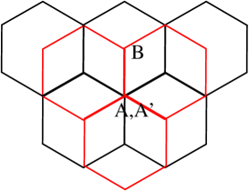
Figure 1: Top view of the arrangement of the Carbon atoms in two neighboring graphene planes in the staggered stacking.

We describe the in-plane electronic properties of graphene using a low energy, long wavelength, expansion around the $K$ and $K^{\prime}$ corners of the 2D Brillouin Zone. This description uses as only input parameter the Fermi velocity, $v_{\rm F}=3ta/2$, where $t$ ($\approx 3$ eV) is the hopping between $\pi$ orbitals located at nearest neighbor atoms, and $a=1.42$Å  is the distance between Carbon atoms. We assume that hopping between planes takes place only between atoms which are on top of each other in neighboring layers. We denote the hopping integral as $t_{\perp}$ ($\approx 0.1t$). The whole model is defined by the parameters $v_{\rm F}$ and $t_{\perp}$. For instance, for the graphene bilayer (the 3D unit cell of the staggered stacking) the Hamiltonian has the form: $H=\sum_{{\bf k}}\Psi^{{\dagger}}({\bf k})H_{0}({\bf k})\Psi({\bf k})$, where ${{\bf k}}=(k_{x},k_{y})$ is the 2D momentum measured relative to the $K$ ($K^{\prime}$) point (we use units such that $c=1=\hbar$),

$$H_{0}({\bf k})=v_{\rm F}\begin{pmatrix}0&ke^{i\phi({\bf k})}&t_{\perp}/v_{\rm F}&0\\ ke^{-i\phi({\bf k})}&0&0&0\\ t_{\perp}/v_{\rm F}&0&0&ke^{-i\phi({\bf k})}\\ 0&0&ke^{i\phi({\bf k})}&0\end{pmatrix},$$ (1)

$\Psi^{{\dagger}}({\bf k})=\bigl{(}c^{{\dagger}}_{\text{A},1,{\bf k}}\;c^{{\dagger}}_{\text{B},1,{\bf k}}\;c^{{\dagger}}_{\text{A},2,{\bf k}}\;c^{{\dagger}}_{\text{B},2,{\bf k}}\bigr{)}$ is the electron spinor creation operator, and $\phi({\bf k})=\tan^{-1}(k_{y}/k_{x})$ is the 2D angle in momentum space.

In the case of the staggered stacking with $2N$ planes, the full Hamiltonian consists of $2N\times 2N$ matrix with $N/2$ blocks with size $4\times 4$ given by (1). The spinor operator is given by creation and annihilation operators for electrons in different planes: $c^{{\dagger}}_{\alpha,n,{\bf k}}$ where $\alpha=A,B$ labels the sublattices in each plane, and $n=1,\cdots,N$ labels the planes. We define the Green’s functions:

$$G^{n}_{\alpha,\beta}({\bf k},t)=-i\langle{\cal T}c_{\alpha,n,{\bf k}}(t)c^{{\dagger}}_{\beta,n,{\bf k}}(0)\rangle\,,$$ (2)

where ${\cal T}$ is the time ordering operator, and its Fourier transform, $G^{n}_{\alpha,\beta}({\bf k},\omega)$, that can be used to calculate the properties of these systems.

It is easy to see from (1) that $G_{A}^{n}(|{\bf k}|,\omega)$ ($\alpha=\beta=\text{A})$ and $G_{B}^{n}(|{\bf k}|,\omega)$ ($\alpha=\beta=\text{B}$), satisfy the equations:

$$\omega G_{A}^{2n}(|{\bf k}|,\omega) = t_{\perp}[G_{A}^{2n-1}(|{\bf k}|,\omega)+G_{A}^{2n+1}(|{\bf k}|,\omega)]$$

$$+ v_{\rm F}|{\bf k}|e^{i\phi_{\bf k}}G_{B}^{2n}(|{\bf k}|,\omega)\,,$$

$$\omega G_{B}^{2n}(|{\bf k}|,\omega) = v_{\rm F}|{\bf k}|e^{-i\phi_{\bf k}}G_{A}^{2n}(|{\bf k}|,\omega)\,,$$

$$\omega G_{A}^{2n+1}(|{\bf k}|,\omega) = t_{\perp}[G_{A}^{2n}(|{\bf k}|,\omega)+G_{A}^{2n+2}(|{\bf k}|,\omega)]$$

$$+ v_{\rm F}|{\bf k}|e^{-i\phi_{\bf k}}G_{B}^{2n+1}(|{\bf k}|,\omega)\,,$$

$$\omega G_{B}^{2n+1}(|{\bf k}|,\omega) = v_{\rm F}|{\bf k}|e^{i\phi_{\bf k}}G_{A}^{2n+1}(|{\bf k}|,\omega)\,.$$ (3)

The phase factors $e^{i\phi_{\bf k}},e^{-i\phi_{\bf k}}$ can be gauged away by a gauge transformation, leading to a set of equations where the odd and even numbered layers are indistinguishable. We can integrate out the $B$ sites in eq.(3), and write an effective equation for $G_{A}(|{\bf k}|,\omega)$:

$$\left[\omega-\frac{(v_{\rm F}|{\bf k}|)^{2}}{\omega}\right]G_{A}^{n}(|{\bf k}|,\omega)=t_{\perp}[G_{A}^{n+1}(|{\bf k}|,\omega)+G_{A}^{n-1}(|{\bf k}|,\omega)]\,,$$ (4)

which is formally equivalent to the tight binding equations which describe a 1D chain with hopping energy $t_{\perp}$ and effective on site energy $(v_{\rm F}|{\bf k}|)^{2}/\omega$. The Green’s function for the $B$ atoms can be obtained from $G_{A}(|{\bf k}|,\omega)$ using the expression:

$$\left[G^{n}_{\alpha,\beta}(|{\bf k}|,\omega)\right]\equiv\left(\begin{array}[]{cc}{G_{A}^{n}(|{\bf k}|,\omega)}^{-1}+\frac{(v_{\rm F}|{\bf k}|)^{2}}{\omega}&v_{\rm F}|{\bf k}|\\ v_{\rm F}|{\bf k}|&\omega\end{array}\right)^{-1}\,,$$ (5)

so that,

$$G_{B}^{n}(|{\bf k}|,\omega)=\frac{1}{\omega}+\frac{(v_{\rm F}|{\bf k}|)^{2}}{\omega^{2}}G_{A}^{n}(|{\bf k}|,\omega)\,.$$ (6)

A sketch of the resulting 1D tight binding model is given in Fig. 2.

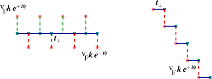
Figure 2: Schematic view of the mapping of the problem of a stack of graphene layers onto a set of one dimensional problems. The hopping between sites are $t_{\perp}$ and $ke^{i\pm\phi}$, where $\phi=\arctan(k_{y}/k_{x})$. Left: staggered stacking. Right: Rhombohedral stacking. Note that the phases $\phi$ can be gauged away in both cases.

In the case of the rhombohedral stacking ($123123\cdots$), a suitable gauge transformation can be used in order to make all layers equivalent, although the two sublattices $A$ and $B$ within each layer remain different, leading to the following set of equations:

$$\omega G^{n}_{A}(\omega) = t_{\perp}G^{n-1}_{B}(\omega)+v_{\rm F}|{\bf k}|G^{n}_{B}(\omega)\,,$$

$$\omega G^{n}_{B}(\omega) = t_{\perp}G^{n+1}_{A}(\omega)+v_{\rm F}|{\bf k}|G^{n}_{A}(\omega)\,,$$ (7)

that determine the properties of the rhombohedral stacking.

In a finite magnetic field $B$ the above equations can be modified with the use of a Peierls substitution ${\bf k}\to{\bf k}+e{\bf A}$, where ${\bf A}$ is the vector potential ($\nabla\times{\bf A}={\bf B}$). In this case, the system breaks into Landau levels that, for a single graphene layer, have energy Peres et al. (2006):

$$E(s,j)=s\omega_{c}\sqrt{j+1}\,,$$ (8)

where $j=0,1,\cdots$ labels the Landau levels, $s=\pm 1$ labels the electron and hole bands,

$$\omega_{c}=\sqrt{2}v_{F}/\ell_{\rm B}=v_{F}\sqrt{2eB}\,,$$ (9)

is the cyclotron frequency, and $l_{B}$ is the cyclotron length.

In the presence of magnetic field we can replace the momentum label ${\bf k}$ by the Landau label $j$ ($|{\bf k}|\to\sqrt{j}/\ell_{\rm B}$) and the extension of the equations (3) become:

$$\omega G_{A}^{2n}(j,\omega)=t_{\perp}[G_{A}^{2n-1}(j,\omega)+G_{A}^{2n+1}(j,\omega)]$$

$$+\frac{v_{\rm F}\sqrt{m}}{\ell_{\rm B}}G_{B}^{2n}(j-1,\omega)\,,$$

$$\omega G_{B}^{2n}(j-1,\omega)=\frac{v_{\rm F}\sqrt{m}}{\ell_{\rm B}}G_{A}^{2n}(j,\omega)\,,$$

$$\omega G_{A}^{2n+1}(j,\omega)=t_{\perp}[G_{A}^{2n}(m,\omega)+G_{A}^{2n+2}(m,\omega)]$$

$$+\frac{v_{\rm F}\sqrt{j+1}}{\ell_{\rm B}}G_{B}^{2n+1}(j+1,\omega)\,,$$

$$\omega G_{B}^{2n+1}(j+1,\omega)=\frac{v_{\rm F}\sqrt{j+1}}{\ell_{\rm B}}G_{A}^{2n+1}(j,\omega)\,.$$ (10)

Note that, in this case, the two inequivalent layers in the unit cell cannot be made equivalent by a gauge transformation as in (3).

In rhombohedral case, the presence of a magnetic field, (7) become:

$$\omega G^{n}_{A}(\omega) = t_{\perp}G^{n-1}_{B}(\omega)+\frac{v_{\rm F}}{\ell_{\rm B}}\sqrt{j}G^{n}_{B}(\omega)\,,$$

$$\omega G^{n}_{B}(\omega) = t_{\perp}G^{n+1}_{A}(\omega)+\frac{v_{\rm F}}{\ell_{\rm B}}\sqrt{j+1}G^{n}_{A}(\omega)\,.$$ (11)

III Stacks of a few graphene layers.

III.1 Generic energy bands.

Using the 1D tight binding mapping discussed in the preceding section, we can write an implicit equation for the eigenenergies of a system with $N$ layers with the staggered stacking as:

$$\epsilon_{{\bf k}}=\frac{(v_{\rm F}|{\bf k}|)^{2}}{\epsilon_{{\bf k}}}+2t_{\perp}\cos\left(\frac{\pi n}{N+1}\right)\,,$$ (12)

where $n=1,\cdots N$, so that the dispersion becomes:

$$\epsilon_{{\bf k}}\!=\!t_{\perp}\!\cos\left(\!\frac{\pi n}{N+1}\!\right)\!\pm\!\sqrt{(v_{\rm F}|{\bf k}|)^{2}\!+\!t_{\perp}^{2}\!\cos^{2}\left(\!\frac{\pi n}{N+1}\!\right)}\,.$$ (13)

III.2 Bilayer.

A number of properties of the present model applied to a graphene bilayer can be found in ref. [McCann and Fal’ko, 2006]. We extend those results here to the case where there is an electrostatic potential which makes the two layers inequivalent. The Hamiltonian reads:

$${\cal H}_{2L}({\bf k})\!\!\equiv\!\!\left(\!\!\!\begin{array}[]{cccc}\Delta&v_{\rm F}|{\bf k}|e^{i\phi_{\bf k}}&t_{\perp}&0\\ v_{\rm F}|{\bf k}|e^{-i\phi_{\bf k}}&\Delta&0&0\\ t_{\perp}&0&-\Delta&v_{\rm F}|{\bf k}|e^{-i\phi_{\bf k}}\\ 0&0&v_{\rm F}|{\bf k}|e^{i\phi_{\bf k}}&-\Delta\end{array}\!\!\!\right)\,,$$ (14)

where the difference in the electrostatic potentials in the two layers is $2\Delta$. For $v_{\rm F}|{\bf k}|\ll\Delta\ll t_{\perp}$, the bands at low energy are given by $\pm\epsilon_{\bf k}$ where:

$$\epsilon_{\bf k}\approx\Delta-\frac{\Delta v_{\rm F}^{2}|{\bf k}|^{2}}{t_{\perp}^{2}}+\frac{v_{\rm F}^{4}|{\bf k}|^{4}}{2\Delta t_{\perp}^{2}}\,.$$ (15)

Hence, the bands show an unusual “mexican hat” dispersion, with extrema at $k_{0}\sim\Delta/v_{\rm F}$ with energy $\epsilon_{vH}=\Delta-\Delta^{3}/t_{\perp}^{2}$. Near these special points, the electronic density of states diverges as:

$$D_{\pm}(\epsilon)\propto\frac{t_{\perp}\sqrt{\Delta}}{v_{\rm F}^{2}\sqrt{\epsilon\mp\epsilon_{vH}}}\,,$$ (16)

which is the divergence seen in 1D systems. In order to understand the reason for this 1D behavior consider the situation where the chemical potential is above (or below) $\epsilon_{vH}$. In this case the Fermi surface looks like a ring (a Fermi ring), as shown in Fig. 3. At large radius $k_{0}$ the ring approaches a 1D dispersion with nested Fermi surfaces, characteristic of 1D systems.

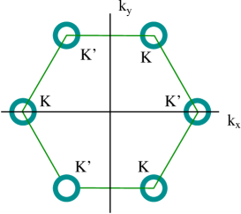
Figure 3: The Fermi ring: the Fermi sea of a biased bilayer.

In the presence of a magnetic field, the Hamiltonian becomes:

$${\cal H}_{2L}(j)\!\!\equiv\!\!\left(\!\!\begin{array}[]{cccc}\Delta&\frac{v_{\rm F}\sqrt{j}}{\ell_{\rm B}}&t_{\perp}&0\\ \frac{v_{\rm F}\sqrt{j}}{\ell_{\rm B}}&\Delta&0&0\\ t_{\perp}&0&-\Delta&\frac{v_{\rm F}\sqrt{j+1}}{\ell_{\rm B}}\\ 0&0&\frac{v_{\rm F}\sqrt{j+1}}{\ell_{\rm B}}&-\Delta\end{array}\!\!\right)\,,$$ (17)

where $j$ is the index of the Landau level. For values of $j$ such that $(v_{\rm F}\sqrt{j})/\ell_{\rm B}\ll\Delta\ll t_{\perp}$, we obtain:

$$\epsilon(j)\!\!=\!\!-\frac{v_{\rm F}^{2}\Delta}{\ell_{\rm B}^{2}t_{\perp}^{2}}\left(\!j\!+\!\frac{1}{2}\!\right)\!\pm\!\sqrt{\Delta^{2}\left(\!1\!-\!\frac{v_{\rm F}^{2}}{2\ell_{\rm B}^{2}t_{\perp}^{2}}\!\right)^{2}\!+\!\frac{v_{\rm F}^{4}j(j+1)}{\ell_{\rm B}^{4}t_{\perp}^{2}}}\,.$$ (18)

III.3 Trilayer.

III.3.1 HOPG stacking (ABA).

The model used here leads to six energy bands in a trilayer. In the absence of electrostatic potentials that break the equivalence of the three layers, we can use eq.(13), to obtain:

$$\epsilon_{\bf k} = \pm v_{\rm F}|{\bf k}|\,,$$

$$\epsilon_{\bf k} = \frac{t_{\perp}\sqrt{2}}{2}\pm\sqrt{\frac{t_{\perp}^{2}}{2}+v_{\rm F}^{2}|{\bf k}|^{2}}\,.$$ (19)

There is a band with Dirac-like linear dispersion, and two more bands which disperse quadratically near $\epsilon=0$, as in a bilayer. The Landau levels, at low energies are:

$$\epsilon(j) = \pm\frac{v_{\rm F}\sqrt{j}}{\ell_{\rm B}}\,,$$

$$\epsilon(j) = \pm\frac{v_{\rm F}^{2}\sqrt{j(j+1)}}{\ell_{\rm B}^{2}t_{\perp}}$$ (20)

Hence, the spectrum can be viewed as a superposition of the corresponding spectrum for the Dirac equation, and that obtained for a bilayer.

The calculation of the energy levels in the presence of electrostatic fields which break the symmetry between the three layers is more complex, and cannot be performed fully analytically. We consider the case when the upper layer is at potential $\Delta$, the lower layer is at potential $-\Delta$, and the middle layer is at zero potential. The Hamiltonian is:

$${\cal H}_{3L}({\bf k})\!\!=\!\!\left(\!\!\begin{array}[]{cccccc}\Delta&v_{\rm F}|{\bf k}|e^{i\phi_{\bf k}}&0&0&0&0\\ v_{\rm F}|{\bf k}|e^{-i\phi_{\bf k}}&\Delta&t_{\perp}&0&0&0\\ 0&t_{\perp}&0&v_{\rm F}|{\bf k}|e^{-i\phi_{\bf k}}&t_{\perp}&0\\ 0&0&v_{\rm F}|{\bf k}|e^{i\phi_{\bf k}}&0&0&0\\ 0&0&t_{\perp}&0&-\Delta&v_{\rm F}|{\bf k}|e^{i\phi_{\bf k}}\\ 0&0&0&0&v_{\rm F}|{\bf k}|e^{-i\phi_{\bf k}}&-\Delta\end{array}\!\!\right)\,,$$ (21)

In the limit $v_{\rm F}|{\bf k}|\ll\Delta\ll t_{\perp}$, one can use perturbation theory to obtain:

$$\epsilon_{\bf k}\approx\frac{\Delta v_{\rm F}|{\bf k}|}{\sqrt{2}t_{\perp}}\left(1-\frac{v_{\rm F}^{2}|{\bf k}|^{2}}{\Delta^{2}}\right)\,.$$ (22)

This equation, although approximate, describes correctly the existence of states at zero energy when $v_{\rm F}|{\bf k}|=\Delta$. The dispersion shows extrema at momenta $k_{0}\propto\Delta/v_{\rm F}$ with energy $\epsilon_{vH}\propto\Delta^{2}/t_{\perp}$, leading to a divergent density of states:

$$D_{\pm}(\epsilon)\propto\frac{\Delta\sqrt{t_{\perp}}}{v_{\rm F}^{2}\sqrt{\epsilon\mp\epsilon_{vH}}}$$ (23)

This expression, as in the case of eq. (16), is typical of 1D systems. The low energy bands of a trilayer with $ABA$ stacking are shown in the upper panel of Fig.[4].

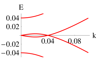
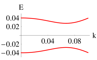
Figure 4: Low energy bands of a trilayer with an electrostatic field which hreaks the equivalence of the three layers (see text). Top: HOPG stacking, $ABA$. Bottom: rhombohedral stacking, $ABC$. The parameters used are $v_{\rm F}=1,t_{\perp}=0.1,\Delta=0.04$.

III.3.2 Rhombohedral stacking (ABC).

The low energy bands of a trilayer with the $ABC$ stacking differ significantly from those for the $ABA$ stacking discussed previously. The $6\times 6$ hamiltonian is:

$${\cal H}_{3L}({\bf k})\equiv\left(\begin{array}[]{cccccc}\Delta&v_{\rm F}|{\bf k}|e^{i\phi_{\bf k}}&0&0&0&0\\ v_{\rm F}|{\bf k}|e^{-i\phi_{\bf k}}&\Delta&t_{\perp}&0&0&0\\ 0&t_{\perp}&0&v_{\rm F}|{\bf k}|e^{i\phi_{\bf k}}&0&0\\ 0&0&v_{\rm F}|{\bf k}|e^{-i\phi_{\bf k}}&0&t_{\perp}&0\\ 0&0&0&t_{\perp}&-\Delta&v_{\rm F}|{\bf k}|e^{i\phi_{\bf k}}\\ 0&0&0&0&v_{\rm F}|{\bf k}|e^{-i\phi_{\bf k}}&-\Delta\end{array}\right)$$ (24)

Assuming that $\Delta\ll t_{\perp}$, only two out of the six $\pi$ bands lie at energies $|\epsilon|\ll t_{\perp}$. These bands are derived from the orbitals at the $B$ sublattice in the two outermost layers, given by the first and sixth entry in eq.(24). One can define an effective $2\times 2$ hamiltonian:

$${\cal H}_{3L\,\,eff}\equiv\left(\begin{array}[]{cc}-\Delta+\frac{\Delta v_{\rm F}^{2}|{\bf k}|^{2}}{t_{\perp}^{2}}&\frac{v_{\rm F}^{3}|{\bf k}|^{3}}{t_{\perp}^{2}}\\ \frac{v_{\rm F}^{3}|{\bf k}|^{3}}{t_{\perp}^{2}}&\Delta-\frac{\Delta v_{\rm F}^{2}|{\bf k}|^{2}}{t_{\perp}^{2}}\end{array}\right)$$ (25)

The dispersion is cubic at low momenta, $\epsilon_{\bf k}\approx(v_{\rm F}|{\bf k}|)^{3}/t_{\perp}^{2}$. The density of states is $D(\epsilon)\propto t_{\perp}^{4/3}/(v_{\rm F}^{2}\epsilon^{1/3})$. The low energ bands of a trilayer with $ABC$ stacking is shown in the lower panel of Fig.[4].

The effective $2\times 2$ hamiltonian in the presence of an applied magnetic field is, for $\Delta=0$:

$${\cal H}_{3L\,\,rhombo}\equiv\left(\begin{array}[]{cc}0&\frac{v_{\rm F}^{3}\sqrt{n(n+1)(n+2)}}{\ell_{\rm B}^{3}t_{\perp}^{3}}\\ \frac{v_{\rm F}^{3}\sqrt{n(n+1)(n+2)}}{\ell_{\rm B}^{3}t_{\perp}^{3}}&0\end{array}\right)$$ (26)

There are, in addition, states localized in the outermost layers, with Landau index $n=0$, and in two layers, with Landau index $n=1$. It is interesting to note that Landau levels associated to different $K$ points are localized in different layers.

IV Semi-infinite stacks of graphene layers.

In this section we consider the case of a graphene multilayer with a surface termination. In the case of the staggered stacking, we can use eq.(3), and obtain for the Green’s function in the bulk as:

$$G_{A}(|{\bf k}|,\omega)=\frac{\omega}{\sqrt{[\omega^{2}-(v_{\rm F}|{\bf k}|)^{2}]-4t_{\perp}^{2}\omega^{2}}}\,.$$ (27)

We can obtain the local density of states by integrating $G_{A}(|{\bf k}|,\omega)$ and $G_{B}(|{\bf k}|,\omega)$ over the parallel momentum ${\bf k}$. This integral can be performed analytically, and we obtain, for the bulk:

$$G_{A}(\omega)\! = \!\frac{\omega}{v_{\rm F}^{2}}\ln\left[\frac{(v_{\rm F}\Lambda)^{2}}{\omega(\omega\!+\!\sqrt{\omega^{2}\!-\!4t_{\perp}^{2}})}\right]\,,$$

$$G_{B}(\omega)\!\!\! = \!\!\!\frac{\sqrt{\omega^{2}\!-\!4t_{\perp}^{2}}}{v_{\rm F}^{2}}\!+\!\frac{\omega}{v_{\rm F}^{2}}\!\ln\!\!\left[\!\frac{(v_{\rm F}\Lambda)^{2}}{\omega(\omega+\sqrt{\omega^{2}-4t_{\perp}^{2}})}\!\right]\!\!.$$ (28)

The local density of states is given by (see also ref. [Nilsson et al., 2006]):

$${\rm Im}G_{A}(\omega) = \frac{\omega}{v_{\rm F}^{2}}\left\{\left[\frac{\pi}{2}+\arctan\left(\frac{\omega}{\sqrt{4t_{\perp}^{2}-\omega^{2}}}\right)\right]\right.$$

$$\times \left.\Theta(2t_{\perp}-\omega)+\pi\Theta(\omega-2t_{\perp})\right\}\,,$$

$${\rm Im}G_{B}(\omega)\!\!\! = \!\!\!\!\left\{\!\!\frac{\sqrt{4t_{\perp}^{2}-\omega^{2}}}{v_{\rm F}^{2}}\!\!+\!\!\frac{\omega}{v_{\rm F}^{2}}\left[\frac{\pi}{2}\!+\!\arctan\left(\!\frac{\omega}{\sqrt{4t_{\perp}^{2}-\omega^{2}}}\right)\!\right]\!\right\}$$ (29)

$$\times \Theta(2t_{\perp}-\omega)+\frac{\pi}{v_{\rm F}^{2}}\Theta(\omega-2t_{\perp})\,.$$

The density of states in the bulk of the staggered stacking is shown in Fig. 5.

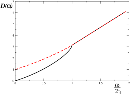
Figure 5: Density of states for the staggered stacking. Continuous line: ${\rm Im}G_{B}(\omega)$. Dashed line: ${\rm Im}G_{A}(\omega)$.

We can use the equivalence to a 1D model for each value of ${\bf k}$, (3) and (7), in order to obtain the Green’s function at the surface layer of a semi-infinite system:

$$G^{\rm surface}_{A}(\omega) = \frac{\sqrt{[\omega^{2}-(v_{\rm F}|{\bf k}|)^{2}]-4t^{2}\omega^{2}}}{2t^{2}\omega}-\frac{\omega}{2t_{\perp}^{2}}\,,$$

$$G^{\rm surface}_{B}(\omega) = \frac{1}{\omega}-\frac{v_{\rm F}^{2}|{\bf k}|^{2}}{\omega^{2}}G^{\rm surface}_{A}(\omega)\,,$$ (30)

for staggered stacking. The local density of states, obtained after integrating these expressions over ${{\bf k}}$ is shown in Fig. 6.

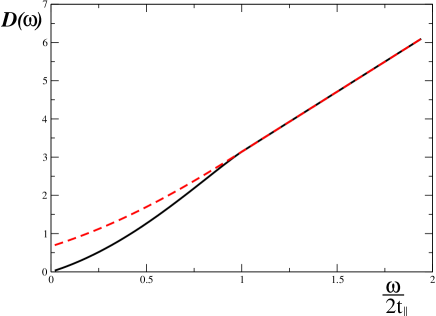
Figure 6: Density of states at the surface layer. Continuous line: ${\rm Im}G_{B}(\omega)$. Dashed line: ${\rm Im}G_{A}(\omega)$.

The 1D tight binding model which describes the electronic bands in rhombohedral graphite (stacking order $123123\cdots$) is given in (7). Using this equation, the Green’s function, integrated over the perpendicular momentum, $k_{\perp}$, is given by:

$$G^{n}({{\bf k}},\omega)\!\!=\!\!\frac{\omega}{\sqrt{\left[\omega^{2}\!-\!(v_{\rm F}|{\bf k}|\!+\!t_{\perp})^{2}\right]\left[\omega^{2}\!-\!(v_{\rm F}|{\bf k}|\!+\!t_{\perp})^{2}\right]}}.$$ (31)

The local density of states can be obtained by integrating this expression over ${\bf k}$:

$${\rm Im}G^{n}(\omega)=\frac{|\omega|}{v_{\rm F}^{2}}\,.$$ (32)

The material, within this approximation, is a semi-metal, with vanishing density of states at the Fermi level at half filling, $\omega=0$. Note that the density of states at low energies is independent of the value of $t_{\perp}$.

In the presence of a magnetic field, we use (11). We can integrate out the Green’s functions for the sites in a given sublattice and obtain:

$$\left(\omega-\frac{t_{\perp}^{2}}{\omega}-\frac{v_{\rm F}^{2}m}{\ell_{\rm B}^{2}\omega}\right)G^{n}_{A}(\omega)=\frac{t_{\perp}v_{\rm F}\sqrt{m}}{\ell_{\rm B}\omega}G^{n-1}_{A}(\omega)$$

$$+\frac{t_{\perp}v_{\rm F}\sqrt{n+1}}{\ell_{\rm B}\omega}G^{n+1}_{A}(\omega)\,.$$ (33)

These equations are formally equivalent to those obtained for the wavefunctions of a displaced 1D harmonic oscillator:

$${\cal H}\equiv\epsilon_{0}+\omega_{0}b^{\dagger}b+g(b^{\dagger}+b)\,,$$ (34)

with the correspondence: $\epsilon_{0}\leftrightarrow t_{\perp}^{2}/\omega$, $\omega_{0}\leftrightarrow v_{\rm F}^{2}/(\ell_{\rm B}^{2}\omega)$, $g\leftrightarrow(t_{\perp}v_{\rm F})/(\ell_{\rm B}\omega)$. The eigenenergies of (34) are $\epsilon_{m}=\epsilon_{0}-g^{2}/\omega_{0}+m\omega_{0}$, and we can write the eigenenergies associated to eq.(11) as:

$$\epsilon_{m}=\frac{t_{\perp}^{2}}{\epsilon_{m}}-\frac{(t_{\perp})^{2}}{\epsilon_{m}}+m\frac{v_{\rm F}^{2}}{\ell_{\rm B}^{2}\epsilon_{m}}\,,$$ (35)

and, finally, we obtain:

$$\epsilon_{m}=\frac{v_{\rm F}\sqrt{m}}{\ell_{\rm B}}\,.$$ (36)

The spectrum, in an applied magnetic field, is discrete, and equal to that in graphene, as well as the local density of states in the absence of the field, eq. (32). The discreteness of the spectrum survives when a stack of rhombohedral graphene is embedded into the staggered stacking, as shown in Fig. 7.

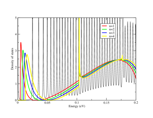
Figure 7: Average density of states of a stack of 50 graphene layers with rhombohedral order, $ABCABC\cdots$, embedded into the staggered stacking, $ABAB\cdots$. The parameters used are: $t_{\perp}=0.1$eV, and $B=1$T ($\ell_{\rm B}\approx 25.7$nm, $v_{\rm F}/\ell_{\rm B}\approx 0.025$eV). The bands of some of the lowest Landau levels of the staggered stacking, calculated for the same parameters, are shown for comparison.

Using the model described in Section II, we obtain for the projected density of states:

$$G^{\rm surface}_{A}(\omega) = \frac{\omega^{2}-t_{\perp}^{2}-(v_{\rm F}|{\bf k}|)^{2}}{2t_{\perp}v_{\rm F}|{\bf k}|\omega}$$

$$- \!\!\frac{\sqrt{\left[\omega^{2}\!-\!(v_{\rm F}|{\bf k}|\!-\!t_{\perp})^{2}\right]\left[\omega^{2}\!-\!(v_{\rm F}|{\bf k}|\!+\!t_{\perp})^{2}\right]}}{2t_{\perp}v_{\rm F}|{\bf k}|\omega}\,,$$

$$G^{\rm surface}_{B}(\omega) = \frac{1}{\omega-(v_{\rm F}|{\bf k}|)^{2}G^{\rm surface}_{A}(\omega)}\,.$$ (37)

The real part of these Green’s functions has a pole at $\omega=0$ for $|{\bf k}|\leq t_{\perp}/v_{\rm F}$, indicating the presence of a surface state. The projected density of states, as function of $|{\bf k}|$, is sketched in Fig. 8.

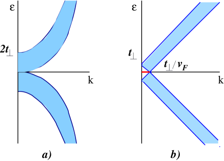
Figure 8: Sketch of the projected density of states at the surface, as function of parallel momentum. Left: staggered stacking. Right: rhombohedral stacking (the line at $\epsilon=0$ stands for a dispersionless band of surface states).

We can also analyze modifications of the surface, induced by electrostatic potentials or local changes of the stacking order. A shift of the topmost layer by a potential $\epsilon$ does not change qualitatively the projected band structure shown in Fig. 8, unless $\epsilon\geq t_{\perp}$. On the other hand, a stacking of the type $1232323\cdots$ leads to a surface band, which can be shifted by an external potential, $\epsilon$, applied to the topmost layer, labeled $1$. As the structure looks like a perfect staggered stacking beyond this layers, and the couplings are local, the Green’s function in the topmost layer is given by:

$$\left[G_{\alpha,\beta}(\omega)\right]\equiv\left(\begin{array}[]{cc}\omega-\epsilon&v_{\rm F}|{\bf k}|\\ v_{\rm F}|{\bf k}|&\left(G_{A}^{{\rm stag.}}\right)^{-1}+\frac{(v_{\rm F}|{\bf k}|)^{2}}{\omega}\end{array}\right)^{-1}$$ (38)

where the labels $A,B$ correspond to the two inequivalent sites in the topmost layer. A sketch of the resulting projected electronic structure is shown in Fig. 9. This result is consistent with the observation of at least two frequencies in the Shubnikov-de Haas experiments in graphene multilayers with induced carriers at the surface reported in ref. [Morozov et al., 2005].

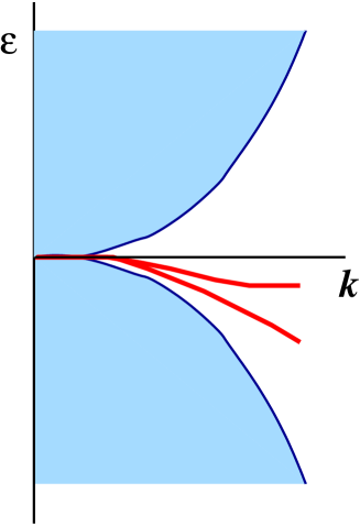
Figure 9: Sketch of the projected density of states of a stack of graphene layers with ordering $CABAB\cdots$, in presence of a potential shift in the topmost layer. The lines outside the continuum of states stand for a two bands of of surface states.

V Conclusions

We have analyzed a minimal model for the electronic structure of stacks of graphene planes, which allows us to obtain a number of interesting results analytically. In the following, we outline some of the most relevant ones:

• Bilayers and trilayers, in the presence of electrostatic fields that break the equivalence of the layers, develop van Hove singularities where the density of states behaves in a quasi 1D fashion, $D(\epsilon)\propto(\epsilon-\epsilon_{vH})^{-1/2}$.

• The Landau levels of a trilayer, in the absence of electrostatic effects, are given by a set of levels which depend on the field in the same way as for a single layer, $\epsilon(j)=\pm(v_{\rm F}\sqrt{j})/\ell_{\rm B}$, and another set which is equivalent to the levels in a bilayer, $\epsilon(j)=\pm((v_{\rm F}^{2}\sqrt{j(j+1)})/t_{\perp}\ell_{\rm B}^{2})$. A comparison of the two sets will allow for an independent measurement of the value of $t_{\perp}$.

• The surface density of states in staggered stacking vanishes at zero energy at the sites with a nearest neighbor in the next layer. This result may explain the difference in the images of the atoms at the two sublattices observed in STM measurements of graphite surfacesTománek and Louie (1988).

• The bulk local density of states of rhombohedral stacking ($ABCABC\cdots$) vanishes at zero energy, and is independent of the value of the interlayer hopping, $t_{\perp}$. The spectrum of bulk Landau levels is discrete, unlike most three dimensional systems, and shows the same field dependence as that of a single graphene layer, with independence of the value of $t_{\perp}$. Hence, discrete, quasi-2D Landau levels may exist in nominally 3D samples, helping to explain the experiments in ref. [Esquinazi et al., 2003].

• The surface of rhombohedral, and of staggered stacking with a rhombohedral termination ($CABAB\cdots$) has surface states, with a well defined dispersion as function of the parallel momentum. This result may help to explain the observation of Shubnikov-de Haas oscillations in graphitic systems with a highly doped surface Morozov et al. (2005).

VI Acknowledgments.

We have benefited from interesting discussions on these topics with C. Berger, P. Esquinazi, W. A. de Heer, A. K. Geim, A. F. Morpurgo, J. Nilsson, K. Novoselov, J. G. Rodrigo, and S. Vieira. A.H.C.N. was supported through NSF grant DMR-0343790. N. M. R. P. thanks ESF Science Programme INSTANS 2005-2010, and FCT under the grant POCTI/FIS/58133/2004. F. G. acknowledges funding from MEC (Spain) through grant FIS2005-05478-C02-01 and the European Union Contract 12881 (NEST).

References

• Novoselov et al. (2004) K. S. Novoselov, A. K. Geim, S. V. Morozov, D. Jiang, Y. Zhang, S. V. Dubonos, I. V. Gregorieva, and A. A. Firsov, Science 306, 666 (2004).
• Zhang et al. (2005a) Y. Zhang, J. P. Small, M. E. S. Amori, and P. Kim, Phys. Rev. Lett. 94, 176803 (2005a).
• Berger et al. (2004) C. Berger, Z. M. Song, T. B. Li, X. B. Li, A. Y. Ogbazghi, R. Feng, Z. T. Dai, A. N. Marchenkov, E. H. Conrad, P. N. First, et al., J. Phys. Chem. B 108, 19912 (2004).
• Bunch et al. (2005) J. S. Bunch, Y. Yaish, M. Brink, K. Bolotin, and P. L. McEuen, Nano Lett. 5, 2887 (2005).
• Novoselov et al. (2005a) K. S. Novoselov, D. Jiang, F. Schedin, T. J. Booth, V. V. Khotkevich, S. V. Morozov, and A. K. Geim, Proc. Nat. Acad. Sc. 102, 10451 (2005a).
• Novoselov et al. (2005b) K. S. Novoselov, A. K. Geim, S. V. Morozov, D. Jiang, M. I. Katsnelson, I. V. Grigorieva, S. V. Dubonos, and A. A. Firsov, Nature 438, 197 (2005b).
• Zhang et al. (2005b) Y. Zhang, Y. W. Tan, H. L. Stormer, and P. Kim, Nature 438, 201 (2005b).
• Novoselov et al. (2006) K. S. Novoselov, E. McCann, S. V. Morozov, V. I. Fal’ko, M. I. Katsnelson, U. Zeitler, D. Jiang, F. Schedin, and A. K. Geim, Nature Physics 2, 177 (2006).
• Morozov et al. (2005) S. V. Morozov, K. S. Novoselov, F. Schedin, D. Jiang, A. A. Firsov, and A. K. Geim, Phys. Rev. B 72, 201401 (2005).
• Nilsson et al. (2006) J. Nilsson, A. H. Castro Neto, F. Guinea, and N. M. R. Peres (2006), eprint cond-mat/0604106.
• Brandt et al. (1988) N. B. Brandt, S. M. Chudinov, and Y. G. Ponomarev, in Modern Problems in Condensed Matter Sciences, edited by V. M. Agranovich and A. A. Maradudin (North Holland (Amsterdam), 1988), vol. 20.1.
• Bacon (1950) G. E. Bacon, Acta Crystalographica 4, 320 (1950).
• Gasparoux (1967) H. Gasparoux, Carbon 5, 441 (1967).
• Rollings et al. (2005) E. Rollings, G.-H. Gweon, S. Y. Zhou, B. S. Mun, B. S. Hussain, A. V. Fedorov, P. N. First, W. A. de Heer, and A. Lanzara (2005), eprint cond-mat/0512226.
• Wallace (1947) P. R. Wallace, Phys. Rev. 71, 622 (1947).
• McClure (1957) J. W. McClure, Phys. Rev. 108, 612 (1957).
• Boyle and Nozières (1958) W. S. Boyle and P. Nozières, Phys. Rev. 111, 782 (1958).
• Slonczewski and Weiss (1958) J. C. Slonczewski and P. R. Weiss, Phys. Rev. 109, 272 (1958).
• McClure (1964) J. W. McClure, IBM J. Res. Dev. 8, 255 (1964).
• Dillon et al. (1977) R. O. Dillon, I. L. Spain, and J. W. McClure, J. Phys. Chem. Sol. 38, 635 (1977).
• Haering (1958) R. R. Haering, Can. Journ. Phys. 36, 352 (1958).
• McClure (1969) J. W. McClure, Carbon 7, 425 (1969).
• Tománek and Louie (1988) D. Tománek and S. G. Louie, Phys. Rev. B 37, 8327 (1988).
• Charlier et al. (1992a) J. C. Charlier, J. P. Michenaud, X. Gonze, and J. P. Vigneron, Phys. Rev. B 44, 4540 (1992a).
• Charlier et al. (1992b) J.-C. Charlier, J.-P. Michenaud, and P. Lambin, Phys. Rev. B 46, 4540 (1992b).
• Charlier et al. (1994) J. C. Charlier, X. Gonze, and J. Michenaud, Carbon 32, 289 (1994).
• Peres et al. (2006) N. M. R. Peres, F. Guinea, and A. H. Castro Neto, Phys. Rev. B. 73, 125411 (2006).
• (28) S. Y. Zhou et al., unpublished.
• McCann and Fal’ko (2006) E. McCann and V. I. Fal’ko, Phys. Rev. Lett. 96, 086805 (2006).
• Esquinazi et al. (2003) P. Esquinazi, D. Spemann, R. Höhne, A. Setzer, K.-H. Han, and T. Butz, Phys. Rev. Lett. 91, 227201 (2003).