Beyond time-dependent exact-exchange:
the need for long-range correlation

Abstract

In the description of the interaction between electrons beyond the classical Hartree picture, bare exchange often yields a leading contribution. Here we discuss its effect on optical spectra of solids, comparing three different frameworks: time-dependent Hartree-Fock, a recently introduced combined density-functional and Green’s functions approach applied to the bare exchange self-energy, and time-dependent exact-exchange within time-dependent density-functional theory (TD-EXX). We show that these three approximations give rise to identical excitonic effects in solids; these effects are drastically overestimated for semiconductors. They are partially compensated by the usual overestimation of the quasiparticle band gap within Hartree-Fock. The physics that lacks in these approaches can be formulated as screening. We show that the introduction of screening in TD-EXX indeed leads to a formulation that is equivalent to previously proposed functionals derived from Many-Body Perturbation Theory. It can be simulated by reducing the long-range part of the Coulomb interaction: this produces absorption spectra of semiconductors in good agreement with experiment.

I Introduction

Density Functional Theory (DFT) Hohenberg and Kohn (1964) is one of the most widely used approaches for the calculation of material properties that are determined by the electronic ground state. Since existing approximations for the in principle exact but in practice unknown exchange-correlation contribution are sometimes not sufficient to obtain the desired accuracy or even qualitative behavior, the search for better functionals is a continuous effort. The same is true concerning neutral electronic excitations that are accessible observables of time-dependent DFT (TD-DFT) Runge and Gross (1984). The failure of most existing approximations for extended systems is in this case even more significant than in the case of the ground state Onida et al. (2002). In both cases, it has been recognized that one may have to accept an additional complication of the functionals in order to get reliable results.

One way to go are orbital-dependent functionals. A local Kohn-Sham (KS) Kohn and Sham (1965) exchange-correlation (xc) potential $v_{xc}$ can be obtained from a given non-local self-energy via the (linearized) Sham-Schlüter equation Sham and Schlüter (1983). This optimized effective potential (OEP) Sharp and Horton (1953) contains much of the important physics of the underlying self-energy. The most prominent approximation along this path is the so-called “exact exchange” (EXX) Görling (2005). The EXX potential $v_{\text{EXX}}$ is obtained as the local counterpart for the non-local Fock operator, which is usually referred to as the “exchange” term. This potential is of course completely different from the original Fock operator: the OEP is local and constructed with KS wavefunctions, whereas the exchange operator is non-local and constructed with Hartree-Fock (HF) wavefunctions. It has been found empirically that EXX eigenvalue band gaps are closer to experimental quasiparticle band gaps than are local-density approximation (LDA) or HF ones. The agreement is very good for simple semiconductors Aulbur et al. (2000a). However, an increasing underestimation for materials with wider band gap has been noticed Magyar et al. (2004). Although EXX contains important effects (it is devoid of self-interaction Görling (2005), as HF is), it is not meant to simulate the effects of Hartree-Fock. In particular, there is no simple interpretation for the KS eigenvalue band gap, no equivalent to the Koopmans theorem. Since KS band gaps are a priori not meant to reproduce experiment, the band gap agreement may arise to a large extent from error cancellations (though still be useful).

Instead, in the case of electronic excitations, the situation is different. Time-Dependent Hartree-Fock (TD-HF) can be understood as an approximation to Many-Body Perturbation Theory (MBPT), obtained from the latter by neglecting correlation. TD-EXX, on the other side, is a straightforward approximation of TD-DFT. Both MBPT and TD-DFT should in principle yield the same (correct) dynamical polarizability, that can be measured e.g. by optical absorption.

HF and, more recently, EXX have been used quite frequently in calculations of real solids Pisani and Dovesi (1980); Rinke et al. (2005), sometimes augmented with approximate correlation functionals, like LDA Aulbur et al. (2000b). Much fewer examples exist instead for their time-dependent counterpart; TD-HF has been carried out for large band gap materials Hanke and Sham (1974), and, to our knowledge, only the absorption spectrum of silicon has been calculated within TD-EXX Kim and Görling (2002a). Intuitively, one would of course not choose TD-HF to calculate, say, the absorption of silicon, since the strong screening in this material can be expected to drastically influence the electron-hole interaction. On the other hand, with EXX KS band gaps comparing so favorably to experiment with respect to their HF counterparts, one may hope for a similar improvement when going from TD-HF to TD-EXX. In fact, it was suggested in Ref. Kim and Görling, 2002a that the TD-EXX absorption spectrum of bulk silicon favorably compares to experiment. It is therefore worthwhile to elucidate the links between the two approaches and discuss differences in the various ingredients as well as in the expected and calculated results. This is the main aim of the present work.

For the sake of clarity and completeness, we add to this comparison a third method, that is to some extent intermediate. This recently introduced approach, called $\rho/G$ in the following, is in fact a combination of MBPT and the density-functional concept Bruneval et al. (2005). As will be discussed below in the exchange-only approximation, it is situated on the same level as HF concerning the quasiparticle band gap, but close to TD-EXX concerning the electron-hole attraction.

The three methods used in the present work are different for some aspects, but tightly linked for others. For a better understanding, we summarize in Table 1 the differences and similarities of the three frameworks. The meaning of the notations and the acronyms will be made clear along this paper.

Our mathematical comparison and numerical results (obtained for the example of bulk silicon) clearly show that in the case of solids all three methods are equivalent. This implies that TD-EXX in its present form is not suitable for the description of absorption spectra of semiconductors. We discuss hence the need for screening of the exchange interaction, and, more precisely, for the screening of the long-range components of it. By introducing the missing terms, we make the link with recently introduced and successfully used functionals derived from Many-Body Perturbation Theory Bruneval et al. (2005); Reining et al. (2002); Adragna et al. (2003); Sottile et al. (2003); Marini et al. (2003), and we discuss which are the most crucially needed corrections.

Table 1: Schematic overview of the different approaches and corresponding observables, approximations and acronyms. Quantities are specified for the exchange-only case.

	(TD-)DFT		$\rho/G$	MBPT
Green’s function	$G_{EXX}(\mathbf{r}_{1}t_{1},\mathbf{r}_{2}t_{2})$		$G_{\text{HF}}(\mathbf{r}_{1}t_{1},\mathbf{r}_{2}t_{2})$	$G_{\text{HF}}(\mathbf{r}_{1}t_{1},\mathbf{r}_{2}t_{2})$
	$\overbrace{\phantom{aaaaaaaaaaaaaaaaaaaaaaaaaaaaaaaaaaaaaaaaaaa}}$
	Lin. Sham-Schlüter	Sham-Schlüter
Potential	$v_{\text{EXX}}$	generally not used	$\Sigma_{x}$	$\Sigma_{x}$
Eigenvalues	$\epsilon_{\text{EXX}}$	generally not used	$\epsilon_{\text{HF}}$	$\epsilon_{\text{HF}}$
Non-interacting response function used in polarizability equation	$\chi_{0}^{\text{EXX}}$		$\chi_{0}^{\text{HF}}$	${}^{4}\chi_{0}^{\text{HF}}$
	$\overbrace{\phantom{aaaaaaaaaaaaaaaaaaaaaaaaaaaaaaaaaaaaaaaaaaa}}$
	Lin. Sham-Schlüter	Sham-Schlüter
Kernel of the Dyson equation	$K^{\text{TD-EXX}}$	$K^{\text{TD-DFT}}$	$K^{\rho/G}$	${}^{4}K(1,2;1^{\prime},2^{\prime})$
consisting of:
Variation of Hartree potential	$v$	$v$	$v$	$\delta(1,1^{\prime})\delta(2,2^{\prime})v(1,2)$
Quasiparticle shift	$f^{(1),\text{lin}}$ ($=F_{\text{EXX}}^{B}$ of Ref. Kim and Görling, 2002a)	$f^{(1)}=\chi_{0}^{\text{EXX}-1}-\chi_{0}^{\text{HF}-1}$	—	—
Electron-hole interaction	$f^{(2),\text{lin}}$ ($=F_{\text{EXX}}^{A}$ of Ref. Kim and Görling, 2002a)	$f^{(2)}=\chi_{0}^{\text{HF}-1}G_{\text{HF}}G_{\text{HF}}vG_{\text{HF}}G_{\text{HF}}\chi_{0}^{\text{HF}-1}$	$f^{(2)}$	$1/i\delta\Sigma_{x}/\delta G_{\text{HF}}={}^{4}v=$ $=\delta(1,2)\delta(1^{\prime},2^{\prime})v(1,1^{\prime})$
Name of the approaches	TD-EXX	Non-lin. TD-EXX	Exchange-only approx. of $\rho/G$	TD-HF
For solids, see papers	Kim and Görling Kim and Görling (2002a)	Bruneval et al Bruneval et al. (2005)	Bruneval et al Bruneval et al. (2005)	Hanke and Sham Hanke and Sham (1974)

II Electron-hole interaction in the quasiparticle and in the density-functional framework

It is useful to first recapitulate the main features of the various approaches that will be compared. For the sake of clarity, we simplify the problem and do not distinguish between KS and HF single-particle wavefunctions in the following. In the numerical examples, we use LDA wavefunctions throughout, and furthermore, all the band structures (LDA, HF, EXX) differ solely by a rigid shift of the band gap. These assumptions are very reasonable for bulk silicon Hybertsen and Louie (1986); Bruneval (2005) (of course, the situation would be rather different in finite systems Baerends and Gritsenko (2005)). Atomic units are used throughout the present work. We often employ the widely spread many-body short-hand notation $1=(\mathbf{r}_{1},t_{1})$ and omit to specify spin explicitly.

The neutral excitations of materials are described by the polarizability or density-density linear response function $\chi({\bf r},{\bf r}^{\prime},t-t^{\prime})$. This quantity expresses the linear response of the electronic density to variations of an external potential $\delta U_{ext}(\mathbf{r}^{\prime},t^{\prime})$:

$$\chi({\bf r},{\bf r}^{\prime},t-t^{\prime})=\left.\frac{\delta\rho(\mathbf{r},t)}{\delta U_{ext}(\mathbf{r}^{\prime},t^{\prime})}\right|_{U_{ext}=0}.$$ (1)

Beside the response of independent particles $\chi_{0}({\bf r},{\bf r}^{\prime},t-t^{\prime})$, the full density-density response function further contains contributions stemming from the self-consistently induced potentials. Independent particle and interacting particle response functions are linked via a Dyson-like polarizability equation, symbolically:

$$\chi=\chi_{0}+\chi_{0}\kappa\chi,$$ (2)

where the kernel $\kappa$ first of all is due to a self-consistently induced Hartree potential $v_{H}^{ind}({\bf r},t)=\int d{\bf r}^{\prime}dt^{\prime}\left[\delta v_{H}({\bf r},t)/\delta\rho({\bf r}^{\prime},t^{\prime})\right]\delta\rho({\bf r}^{\prime},t^{\prime})$. The induced Hartree potential contributes hence to the kernel $\kappa$ with the simple term $\left[\delta v_{H}({\bf r},t)/\delta\rho({\bf r}^{\prime},t^{\prime})\right]=v({\bf r}-{\bf r}^{\prime})\delta(t-t^{\prime})$.

A similar variation has to be added for the exchange-correlation potential. In the TD-DFT framework, this leads to the exchange-correlation kernel $f_{xc}({\bf r},{\bf r}^{\prime},t-t^{\prime})=\left[\delta v_{xc}({\bf r},t)/\delta\rho({\bf r}^{\prime},t^{\prime})\right]$, and Eq. (2) is an integral equation for $\chi({\bf r},{\bf r}^{\prime},t-t^{\prime})$:

$$\chi(1,2)=\chi_{0}^{\text{KS}}(1,2)+\int d3d4~{}\chi_{0}^{\text{KS}}(1,3)K^{\text{TD-DFT}}(3,4)\chi(4,2).$$ (3)

Here, $K^{\text{TD-DFT}}(3,4)=v(3,4)+f_{xc}(3,4)$. $v(1,2)=v(\mathbf{r}_{1}-\mathbf{r}_{2})\delta(t_{1}-t_{2})$ stands for the instantaneous bare Coulomb interaction and $\chi_{0}^{\text{KS}}$ is the Kohn-Sham independent-particle response function.

In the MBPT framework, the equivalent variation has to be calculated for the non-local exchange-correlation self-energy $\Sigma$. As a consequence, it is not possible to obtain straightforwardly a closed Dyson-like equation for the two-point density response function. This remains also true in the HF approximation, where $\Sigma$ reduces to the – still non-local – Fock operator $\Sigma_{x}$. Moreover, the exchange term has a simple dependence on the one-particle Green’s function $G(\mathbf{r}_{1}t,\mathbf{r}_{2}t^{+})$ [not so simple on the density $\rho({\bf r})$]. Therefore, as in the general case, the derivation of a closed equation for the response function of the Hartree-Fock system leads to the introduction of four-point polarizabilities ${}^{4}\chi_{0}$ and ${}^{4}\chi$: Onida et al. (2002)

$${{}^{4}}\chi(1,2;1^{\prime},2^{\prime})={{}^{4}}\chi_{0}(1,2;1^{\prime},2^{\prime})+\int d3d4d5d6~{}{{}^{4}}\chi_{0}(1,3;1^{\prime},4){{}^{4}}K(3,6;4,5){{}^{4}}\chi(5,2;6,2^{\prime}).$$ (4)

[Contracting indices to ${}^{4}\chi(1,2;1,2)$ gives back the usual $\chi(1,2)$.] This equation is the Bethe-Salpeter equation Hanke and Sham (1979); Onida et al. (2002).

For the Hartree-Fock case, the kernel ${}^{4}K$ is

$${{}^{4}}K(3,6;4,5)=2\delta(3,4)\delta(5,6)v(3,5)-\delta(3,6)\delta(4,5)v(3,4).$$ (5)

The first $v$ of the kernel stems from the variation of the Hartree potential (with a factor of 2 for singlet excitons), and the second $v$, from the variation $[\delta\Sigma_{x}/\delta G]$ of the Fock exchange operator $\Sigma_{x}$. ${{}^{4}}\chi_{0}$, the 4-point independent-quasiparticle polarizability, is constructed here using HF eigenvalues, ${{}^{4}}\chi_{0}^{\text{HF}}$ (see last column of Table 1). Note that beyond bare exchange, in most applications of the Bethe-Salpeter equation a statically screened Coulomb interaction $W$ replaces $v$ in the second term Onida et al. (2002). This term gives rise to a direct screened electron-hole attraction instead of the unscreened one in the case of HF.

Recently, Bruneval et al. Bruneval et al. (2005) introduced a general formulation that avoids the solution of the four-point Bethe-Salpeter equation. This approach (named $\rho/G$ here) is based on the use of the density-functional concept within Hedin’s equation of MBPT Hedin (1965). Of interest here, it yields an explicit formula for the two-point polarizability $\chi$ that contains all exchange-correlation effects via the density-variation of the self-energy, $\delta\Sigma/\delta\rho$, and via the explicit use of an independent-quasiparticle (QP) polarizability. The approach is between TD-DFT [because it leads to a two-point polarizability equation like Eq. (3)] and MBPT (because the QP, instead of the KS, independent-particle response appears). Using the $GW$ approximation for $\Sigma$ Hedin (1965) and some further straightforward approximations, this approach leads to previously proposed equation for $\chi$ that yields spectra in excellent agreement with the spectra calculated from Bethe-Salpeter equation, and consequently, with experimental spectra Reining et al. (2002); Adragna et al. (2003); Sottile et al. (2003); Marini et al. (2003). This equation is similar to Eq. (4), but recast into a two-point form:

$$\chi(1,2)=\chi_{0}(1,2)+\int d3d4~{}\chi_{0}(1,3)K^{\rho/G}(3,4)\chi(4,2),$$ (6)

where the two-point kernel $K^{\rho/G}$ reads

$$K^{\rho/G}(1,2) := v(1,2)+f^{(2)}(1,2)$$ (7)

$$= v(1,2)-i\int d3d4d5~{}\chi_{0}^{-1}(13)G(34)G(53)\frac{\delta\Sigma(45)}{\delta\rho(2)}.$$ (8)

For the present work, it is interesting to choose the Fock operator as an approximation for the self-energy in $\delta\Sigma/\delta\rho$, and consistently, to use the HF independent-particle response function $\chi_{0}^{\text{HF}}$ for $\chi_{0}$ in the polarizability equation (second column of Table 1). The two-point kernel $K^{\rho/G}$ of the Hartree-Fock problem becomes, following Ref. Bruneval et al., 2005,

$$K^{\rho/G}(1,2)\simeq v(1,2)+\int d3d4d5d6~{}\chi_{0}^{\text{HF}-1}(13)G_{\text{HF}}(34)G_{\text{HF}}(53)v(45)G_{\text{HF}}(46)G_{\text{HF}}(65)\chi_{0}^{\text{HF}-1}(62),$$ (9)

where $G_{\text{HF}}(1,2)$ is the HF Green’s function and hence $\Sigma_{x}=iG_{\text{HF}}v$ the Fock operator. Here, as in Ref. Bruneval et al., 2005, we have used the approximation $\delta G/\delta\rho=-G(\delta G^{-1}/\delta\rho)G\simeq G\chi_{0}^{-1}G$.

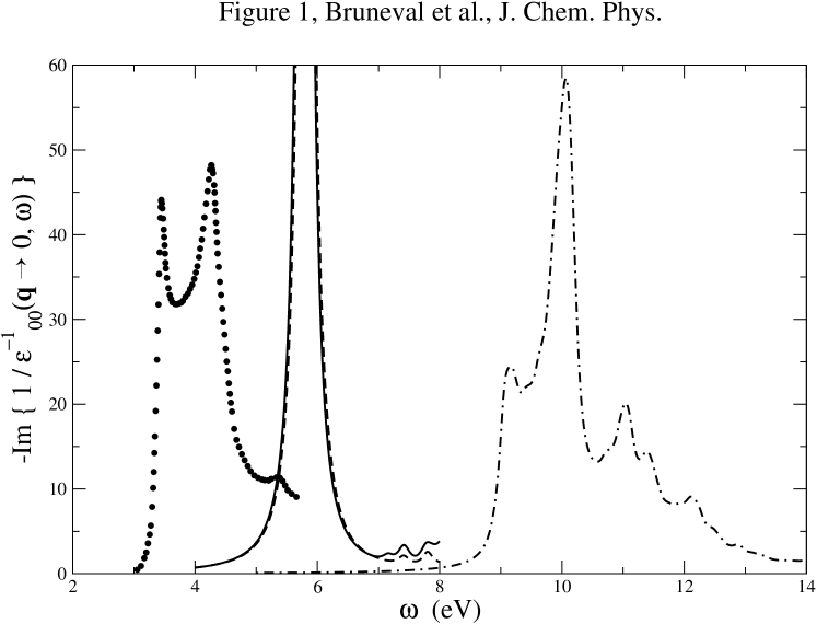
Figure 1: Imaginary part of the macroscopic dielectric function of bulk silicon. Continuous curve: TD-HF result; dashed line: $\rho/G$ result (see text) from Ref. Bruneval et al., 2005; dot-dashed curve: independent-HF-QP result (see text); circles: experiment Lautenschlager et al. (1987).

One may wonder whether Eq. (6) using this approximate $\rho/G$ kernel is indeed able to reproduce TD-HF. Fig. 1 compares the TD-HF (continuous curve) and $\rho/G$ (dashed curve) calculated absorption spectra for bulk silicon. Of course, the results are far from any experiment: the HF direct band gap of silicon is 8.92 eV [see the independent-HF-QP result, dot-dashed curve obtained from $\text{Im}(\chi_{0})$], more than twice the experimental QP direct band gap of 3.40 eV Landolt-Börnstein (1982). Also the electron-hole attraction is drastically overestimated due to the absence of screening, and a strongly bound exciton is formed inside the HF-QP band gap. Finally, QP and excitonic errors cancel to a large extent; the absorption spectrum falls in an energy region that is closer to the experimental one (circles) Lautenschlager et al. (1987), but the lineshape is of course completely wrong. This is to be expected and is not the point here. Instead, it is noteworthy to point out that the TD-HF [Eqs. (4) and (5)] and $\rho/G$ [Eqs. (6) and (9)] results are almost indistinguishable, as it was the case in previous findings when correlation beyond Hartree-Fock was taken into account Sottile et al. (2003) and the effective interaction was therefore much weaker. This means that the kernel $f^{(2)}$ in Eq. (9) simulates well the TD-HF bare electron-hole attraction.

Let us now come to a fully TD-DFT formulation of the problem (see the first column of Table 1). This can also easily be written starting from the equations of Ref. Bruneval et al., 2005: indeed, that work showed that a differentiation of the time-dependent Sham-Schlüter condition van Leeuwen (1996) (that the TD-DFT and the MBPT time-dependent densities correspond) with respect to the density yields the TD-DFT polarizability equation,

$$\chi(1,2)=\chi_{0}^{\text{KS}}(1,2)+\int d2d3~{}\chi_{0}^{\text{KS}}(1,3)K^{\text{TD-DFT}}(3,4)\chi(4,2),$$ (10)

in which now the KS independent-particle response $\chi_{0}^{\text{KS}}$ appears, and the corresponding kernel reads $K^{\text{TD-DFT}}=K^{\rho/G}+(\chi_{0}^{\text{KS}-1}-\chi_{0}^{-1})$. In other words, the TD-DFT kernel has, with respect to the $\rho/G$ one, an additional contribution $f^{(1)}:=\chi_{0}^{\text{KS}-1}-\chi_{0}^{-1}$. If inserted in a Dyson-like polarizability equation, $f^{(1)}$ transforms the KS independent-particle response $\chi_{0}^{\text{KS}}$ into the corresponding QP independent-particle response $\chi_{0}$. It essentially opens the band gap from the KS to the QP one Bruneval et al. (2005); Stubner et al. (2004).

When applied to the exchange-only case, one obtains hence $K^{\text{TD-DFT}}=v+f^{(1)}+f^{(2)}$ where $f^{(1)}$ has the role to open the band gap to the HF one, and the bare electron-hole attraction $f^{(2)}$ is the kernel of Eq. (7) [approximated e.g. by Eq. (9)]. We call this approach the “non-linearized TD-EXX approach”, as opposed to the standard TD-EXX approach that will be discussed in the next section.

It is quite obvious to see that Eq. (10) and Eq. (6) yield identical results, as we have also confirmed numerically (without displaying the result here). This leads to an important conclusion of this section, namely: non-linearized TD-EXX reproduces TD-HF. The band gap difference between EXX and HF is cancelled in the optical spectrum by the contribution $f^{(1)}$ to the kernel, whereas the effect of the electron-hole attractions $\delta\Sigma_{x}/\delta G$ and $f^{(2)}$ are extremely close.

III Time-dependent Hartree-Fock and time-dependent exact exchange

Let us now make the link to what is usually called “TD-EXX”. The starting point is the linearized Sham-Schlüter equation, van Leeuwen (1996)

$$i\int d1~{}v_{\text{EXX}}(1)\chi_{0}^{\text{EXX}}(1,2)=\int d1d3\int d4~{}G_{\text{EXX}}(1,3)\Sigma_{x}(3,4)G_{\text{EXX}}(4,2),$$ (11)

where only EXX KS quantities are used to build response functions and the Fock operator $\Sigma_{x}=iG_{\text{EXX}}v$ (the solution of the static version of this equation would yield the static OEP potential $v_{\text{EXX}}$). The functional derivative with respect to the density of $v_{\text{EXX}}$ has a contribution that stems from the derivative of $\Sigma_{x}$ (this is explicitly shown in appendix A),

$$f^{(2),\text{lin}}(1,2)=\int d3d4d5d6~{}\chi_{0}^{\text{EXX}-1}(1,3)G_{\text{EXX}}(3,4)G_{\text{EXX}}(5,3)v(4,5)G_{\text{EXX}}(4,6)G_{\text{EXX}}(6,5)\chi_{0}^{\text{EXX}-1}(6,2).$$ (12)

This term is very similar to $f^{(2)}$ in Eq. (9). Since we do not distinguish single-particle wavefunctions, the only difference lies in the eigenvalues used to build all the Green’s functions, and $\chi_{0}$.

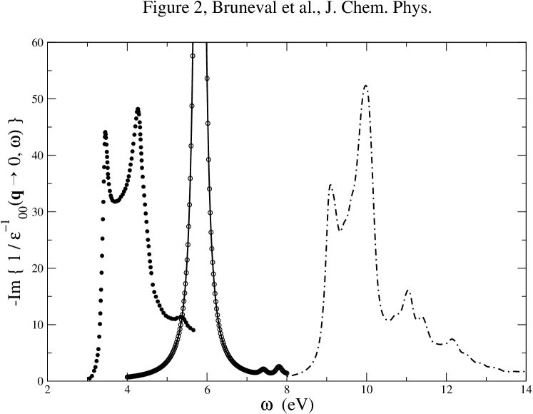
Figure 2: Imaginary part of the macroscopic dielectric function of bulk silicon. Continuous curve: $\rho/G$ result (see text) using $f^{(2)}$; open circles: $\rho/G$ result using $f^{(2),\text{lin}}$ [this corresponds to TD-EXX (see text)]; dot-dashed curve: using $f^{(2),\text{lin}}$ and the modified Coulomb interaction of Ref. Kim and Görling, 2002a.

Actually, it turns out that this difference is not significant. Fig. 2 shows a comparison of the $\rho/G$ spectrum calculated using $f^{(2)}$ and $f^{(2),\text{lin}}$, respectively (continuous line and open circles). The reason for this perfect agreement is a strong cancellation between energy denominators in the inverse response functions and the two Green’s functions in terms of the type $GG\chi_{0}^{-1}$.

It is now important to notice that $f^{(2),\text{lin}}$ is nothing else but the electron-hole attraction term of TD-EXX. This term corresponds precisely to the terms $H_{X}^{1}$ and $H_{X}^{2}$ in Ref. Kim and Görling, 2002b (see appendix B for a detailed derivation). Hence, we find a strongly overbound exciton from the TD-EXX electron-hole attraction.

The rest of the terms that stem from the derivative of Eq. (11) is the linearized version of $f^{(1)}$. It reads (see appendix A)

$$f^{(1),\text{lin}}(1,2)=\int d3d4d5d6~{}\chi_{0}^{\text{EXX}-1}(1,3)G_{\text{EXX}}(3,6)G_{\text{EXX}}(6,4)\left[\Sigma_{x}(4,5)-\delta(4,5)v_{\text{EXX}}(4)\right]G_{\text{EXX}}(5,3)\chi_{0}^{\text{EXX}-1}(6,2)\\ +\int d3d4d5d6~{}\chi_{0}^{\text{EXX}-1}(1,3)G_{\text{EXX}}(6,3)G_{\text{EXX}}(3,4)\left[\Sigma_{x}(4,5)-\delta(4,5)v_{\text{EXX}}(4)\right]G_{\text{EXX}}(5,6)\chi_{0}^{\text{EXX}-1}(6,2).$$ (13)

As shown in appendix B, this expression (again assuming that KS and HF wavefunctions are equal) corresponds to the terms $H_{X}^{3}$ and $H_{X}^{4}$ of Ref. Kim and Görling, 2002b.

$f^{(1)}$ has the difficult task to shift the whole independent-particle spectrum above the HF band gap, and it turns out that it is more delicate to linearize this contribution than $f^{(2)}$. It is clear that the linearization of $f^{(1)}$ cannot, by miracle, cancel the overestimate of the exciton binding in $f^{(2)}$: in the best case (met for few transitions), $f^{(1),\text{lin}}$ is a good approximation to $f^{(1)}$ and rigidly shifts the whole spectra conserving the shape (and therefore the bound exciton); otherwise, $f^{(1),\text{lin}}$ is numerically instable and gives rise to scattered spectra T (1). Therefore, in the following calculations, we always use the non-linearized version $f^{(1)}$ (instead of $f^{(1),\text{lin}}$). For the same reason, it is not astonishing that Kim and Görling have found a “collapse” of the silicon absorption spectrum Kim and Görling (2002a). The authors have solved the problem by cutting off the long-range (small-$q$) part of the Coulomb interaction. In fact, this procedure leads to drastic changes in the spectrum: we have repeated their calculation by introducing the same cutoff in $f^{(2)}$. Now, instead of the strongly bound exciton we find a lineshape in good agreement with experiment, as can be seen by the dot-dashed curve in Fig. 2. ($f^{(1)}$ has not been modified; therefore the spectrum stays in the HF energy region.) In the same way, the reduction of the long-range Coulomb interaction in $f^{(1)}$ translates into a shift of the spectrum towards the experimental position.

This result may seem rather ad hoc. However, it can be understood and used to improve the approach, as we will discuss in the following section.

IV Correlation contributions

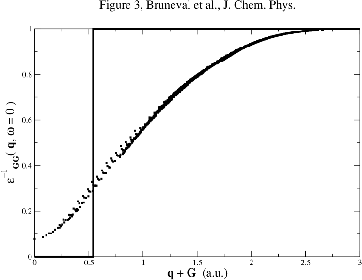
Figure 3: Diagonal of the static inverse RPA dielectric function of bulk silicon. The vertical line denotes the border of the Brillouin zone.

Fig. 3 shows the diagonal of the static inverse dielectric matrix $\epsilon_{\mathbf{G},\mathbf{G}}^{-1}(\bf q)$ of bulk silicon as a function of $|\bf q+\bf G|$, calculated in the Random Phase Approximation (RPA). The vertical line denotes the border of the Brillouin zone, up to which Kim and Görling Kim and Görling (2002a) have chosen to set the Coulomb interaction to zero. The step function that one obtains in this way can be seen as a first reasonable approximation for the full screening curve. In other words, the modified Coulomb interaction is an approximation to the screened Coulomb interaction $W$: it compensates for the lack of correlation. Hence, the impressingly good result of Kim and Görling and in Fig. 2 can be explained: the new, screened $f^{(2)}$ is just an approximation to the electron-hole attraction term derived in Refs. Reining et al., 2002; Adragna et al., 2003 from the Bethe-Salpeter equation, which it reproduces in the same way as the unscreened version reproduces TD-HF. The same applies in principle to $f^{(1)}$.

It should be pointed out that the good results obtained from the more sophisticated approaches Reining et al. (2002); Adragna et al. (2003) like $\rho/G$ Bruneval et al. (2005) rely in practice on a number of approximations that are commonly made in the Bethe-Salpeter approach from which they are derived. In particular, QP eigenvalues are calculated within the $GW$ approximation (including dynamical effects), whereas $W$ for the electron-hole screening is taken static. Although these are much less crude approximations than the cutoff used above for TD-EXX, the search for a perfectly rigorous, but still efficiently working approach is not yet completed.

At present, however, one may be with no doubts satisfied with the precision and reliability of the screened approaches Reining et al. (2002); Adragna et al. (2003); Sottile et al. (2003); Marini et al. (2003). Nevertheless, it is interesting to investigate the role of correlation further, since the cutoff approach of Kim and Görling gives precious hints: the screening of the long-range (small-$q$) part of $v$ is seen to have drastic effects. This is consistent with other studies of the long-range contribution of the exchange-correlation kernel in bulk materials (see e.g. Refs. Botti et al., 2004; de Boeij et al., 2001).

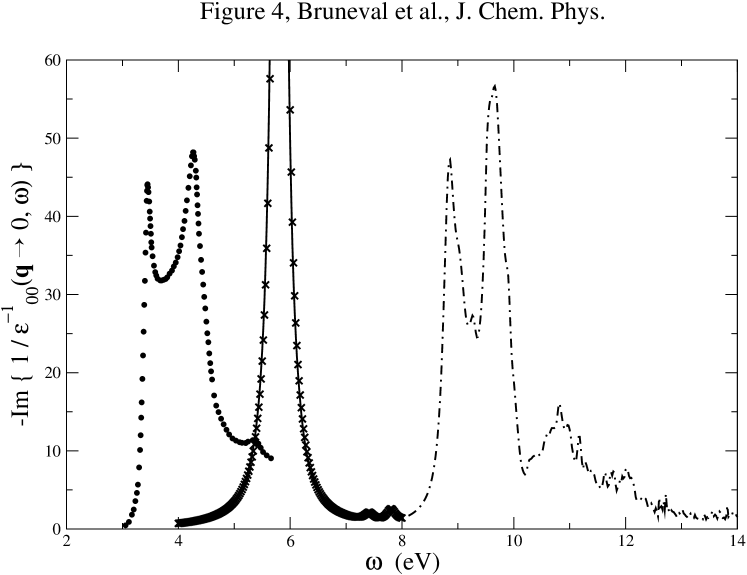
Figure 4: Imaginary part of the macroscopic dielectric function of bulk silicon. Continuous curve: non-linearized TD-(EXX+cLDA) result; stars: non-linearized TD-EXX result; dot-dashed curve: using $f^{(2),\text{lin}}$ and the modified Coulomb interaction $v/6$.

Without considering these findings, one might hope to introduce correlation in another, more standard way, namely by adding LDA correlation to EXX as it is quite frequently done for the ground state potential Aulbur et al. (2000b). Fig. 4 shows the result of a TD-(EXX+cLDA) calculation (continuous curve) as compared to the TD-EXX result (stars): the LDA correlation does not give rise to any visible changes. (Note that in both cases $f^{(1),\text{lin}}$ has been replaced by the corresponding $f^{(1)}$, for clarity. In other words, only the effect of correlation in $f^{(2)}$ is tested.)

The adiabatic LDA kernel is in fact short ranged, and cannot suppress the overbound exciton stemming from long-range contributions. Instead, as can be seen from the cutoff result, any model $\epsilon^{-1}$ that reasonably screens the long range contributions can do the job; for illustration, we also show in Fig. 4 the result obtained replacing $v$ by $v/\langle\epsilon_{0}\rangle$ in $f^{(2),lin}$, where $\langle\epsilon_{0}\rangle$ is taken to be an average dielectric constant of 6 for silicon. In spite of the extreme simplicity of the treatment of correlation, the result is again satisfactory (note that, as in Fig. 2, the unscreened $f^{(1)}$ is used; hence, the spectrum results too high in energy). This leaves the hope that, starting from some screened version of TD-EXX and along the lines of Refs. Reining et al., 2002; Adragna et al., 2003; Sottile et al., 2003; Marini et al., 2003; Tokatly and Pankratov, 2001, it is possible to find approximations to TDDFT, less rigorous than TD-EXX, but exempt from its severe shortcomings concerning the description of bulk materials, and that the method is still numerically advantageous with respect to the solution of the Bethe-Salpeter equation. Hybrid functionals like the ones discussed in Ref. Heyd et al., 2005 may be seen as a possibility in this context.

V Conclusions

A time-dependent OEP procedure constructs TD-DFT kernels that yield the same time-dependent density as a given approximation to the self-energy, via a time-dependent Sham-Schlüter equation. Apart from a linearization, this relation is exact. It is therefore not surprising that a careful time-dependent OEP calculation reproduces the solution of the Bethe-Salpeter equation, within the corresponding approximation. The present work verified this agreement for the case of the Hartree-Fock approximation to the self-energy. In particular, the non-linearized and the usual linearized TD-EXX are shown to reproduce the TD-HF calculation and consequently, fail crudely to describe absorption spectra of semiconductors, because the electron-hole interaction is largely overestimated there. We show that TD-EXX gives rise to a huge bound exciton for bulk silicon. The linearization does not cure this shortcoming. The similarity between TD-HF and TD-EXX can also be noticed in the evaluation of vertical excitation energies of finite systems Hirata et al. (2002).

Whatever the approach used, Bethe-Salpeter equation, $\rho/G$ method, or TD-DFT, the inclusion of the screening of the exchange operator is evidenced as crucial to give a proper account for the electron-hole interaction. In particular, the long-range components of the exchange kernel have to be reduced. Furthermore, we demonstrate that the details of the screening do not matter much: two very different and crude models (a cutoff as used by Kim and Görling or a uniformly reduced Coulomb interaction $v/6$) allow us to equally produce realistic absorption spectra of silicon.

The hope of describing optical absorption spectra of semiconductors within TD-DFT is well founded. However, in the framework of unscreened methods, like TD-EXX is, there is no chance to get something else than the disastrous TD-HF results: one has to go beyond TD-EXX. A rigorous OEP method based on “exact screened exchange” may do the job. Fortunately, the inclusion of screening within rather simple approximations, e.g. using an empirically screened Coulomb interaction, seems to be already sufficient.

Appendix A Derivation of the TD-DFT kernels from the linearized TD-Sham Schlüter equation

The present appendix provides the derivation of the linearized TD-EXX kernels from the linearized TD-Sham-Schlüter equation. The linearized TD-Sham-Schlüter equation reads

$$\int d3~{}G_{\text{EXX}}(1,3)v_{\text{EXX}}(3)G_{\text{EXX}}(3,1)=\int d3d4~{}G_{\text{EXX}}(1,3)\Sigma_{x}(3,4)G_{\text{EXX}}(4,1).$$ (14)

When Eq. (14) is differentiated with respect to the TD density $\rho(2)$, we get

$$\int d3~{}G_{\text{EXX}}(1,3)\frac{\delta v_{\text{EXX}}(3)}{\delta\rho(2)}G_{\text{EXX}}(3,1)=\int d3d4~{}G_{\text{EXX}}(1,3)\frac{\delta\Sigma_{x}(3,4)}{\delta\rho(2)}G_{\text{EXX}}(4,1)\\ +\int d3d4~{}\frac{\delta G_{\text{EXX}}(1,3)}{\delta\rho(2)}\left[\Sigma_{x}(3,4)-\delta(3,4)v_{\text{EXX}}(3)\right]G_{\text{EXX}}(4,1)\\ +\int d3d4~{}G_{\text{EXX}}(1,3)\left[\Sigma_{x}(3,4)-\delta(3,4)v_{\text{EXX}}(3)\right]\frac{\delta G_{\text{EXX}}(4,1)}{\delta\rho(2)}.$$ (15)

The linearized exchange operator is simply $\Sigma_{x}(1,2)=iG_{\text{EXX}}(1,2)v(1,2)$. Therefore, the only quantity needed to carry on the derivation is the derivative of $G_{\text{EXX}}$ with respect to $\rho$. It can be evaluated along the following lines, using standard functional analysis relations, and introducing the total KS potential within EXX $v_{\text{KS}}$,

$$\frac{\delta G_{\text{EXX}}(1,2)}{\delta\rho(3)} = \int d4~{}\frac{\delta G_{\text{EXX}}(1,2)}{\delta v_{\text{KS}}(4)}\frac{\delta v_{\text{KS}}(4)}{\delta\rho(3)}$$ (16)

$$= -\int d4d5d6~{}G_{\text{EXX}}(1,5)G_{\text{EXX}}(6,2)\frac{\delta G_{\text{EXX}}^{-1}(5,6)}{\delta v_{\text{KS}}(4)}\frac{\delta v_{\text{KS}}(4)}{\delta\rho(3)}$$

$$= \int d4~{}G_{\text{EXX}}(1,4)G_{\text{EXX}}(4,2)\chi_{0}^{\text{EXX}-1}(4,3),$$

where the last line was obtained from the Dyson equation $G_{\text{EXX}}^{-1}=G_{0}^{-1}-v_{\text{KS}}$ ($G_{0}$ standing for the free-electron Green’s function) and from the definition $\chi_{0}^{\text{EXX}-1}=\delta v_{\text{KS}}/\delta\rho$.

Finally, by inserting Eq. (16) into Eq. (15), by multiplying by $\chi_{0}^{\text{EXX}}(2,5)$, and integrating over the variable 2, we obtain the central equation for the linearized TD-EXX kernel $f^{\text{EXX, lin}}=\delta v_{\text{EXX}}/\delta\rho$:

$$\int d2d3~{}\chi_{0}^{\text{EXX}}(1,3)f^{\text{EXX,lin}}(3,2)\chi_{0}^{\text{EXX}}(2,5)=\int d3d4~{}G_{\text{EXX}}(1,3)G_{\text{EXX}}(4,1)v(3,4)G_{\text{EXX}}(3,5)G_{\text{EXX}}(5,4)\\ -iG_{\text{EXX}}(1,5)\int d3d4~{}G_{\text{EXX}}(5,3)\left[\Sigma_{x}(3,4)-\delta(3,4)v_{\text{EXX}}(3)\right]G_{\text{EXX}}(4,1)\\ -iG_{\text{EXX}}(5,1)\int d3d4~{}G_{\text{EXX}}(1,3)\left[\Sigma_{x}(3,4)-\delta(3,4)v_{\text{EXX}}(3)\right]G_{\text{EXX}}(4,5),$$ (17)

with $\chi_{0}^{\text{EXX}}=-iG_{\text{EXX}}G_{\text{EXX}}$. The kernel $f^{\text{EXX, lin}}$ can be split into two pieces $f^{(1),\text{lin}}$ and $f^{(2),\text{lin}}$, the definitions of which stand respectively in Eqs. (13) and (12). This partition is natural when looking at the analytical form of the terms. It is further physically-driven, since the term $f^{(2),\text{lin}}$ accounts for electron-hole interaction and the term $f^{(1),\text{lin}}$ for the quasiparticle shift. Bruneval et al. (2005); Stubner et al. (2004)

Appendix B Link to TD-EXX

This appendix shows that the kernel obtained in the previous appendix is precisely the EXX kernel of Kim and Görling Kim and Görling (2002b). For simplification, let us name $T^{(1a),\text{lin}}$ the first term of $\chi_{0}^{\text{EXX}}f^{(1),\text{lin}}\chi_{0}^{\text{EXX}}$, $T^{(1b),\text{lin}}$ the second one, and $T^{(2),\text{lin}}=\chi_{0}^{\text{EXX}}f^{(2),\text{lin}}\chi_{0}^{\text{EXX}}$.

We are about to introduce the expression of $G_{\text{EXX}}$ in the previous terms in order to recover all the sixteen terms of Kim and Görling’s kernel. The time-ordered EXX Green’s function $G_{\text{EXX}}$ in frequency domain is

$$G_{\text{EXX}}(\mathbf{r}_{1},\mathbf{r}_{2},\omega)=\sum_{i}\frac{\phi_{i}(\mathbf{r}_{1})\phi_{i}^{*}(\mathbf{r}_{2})}{\omega-\epsilon_{i}-i\eta(2f_{i}-1)},$$ (18)

where $\phi_{i}$ and $\epsilon_{i}$ are the EXX KS wavefunctions and energies for index $i$ (that contains also the $\mathbf{k}$ point information). $f_{i}$ is 1 for occupied states and 0 for empty states.

B.1 Evaluation of $T^{(2),\text{lin}}$

Let us first proceed with the electron-hole interaction term $T^{(2),\text{lin}}$. It reads, after Fourier transform to frequency domain,

$$T^{(2),\text{lin}}(\mathbf{r}_{1},\mathbf{r}_{5},\omega)=\frac{2}{(2\pi)^{2}}\sum_{ijkl}\phi_{i}(\mathbf{r}_{1})\phi_{j}^{*}(\mathbf{r}_{1})\int d\omega_{1}\frac{1}{(\omega+\omega_{1}-\epsilon_{i})(\omega_{1}-\epsilon_{j})}\\ \times\langle ik|v|jl\rangle\phi_{k}^{*}(\mathbf{r}_{5})\phi_{l}(\mathbf{r}_{5})\int d\omega_{2}\frac{1}{(\omega+\omega_{2}-\epsilon_{k})(\omega_{2}-\epsilon_{l})},$$ (19)

as the products in time space become convolutions of frequencies. The factor 2 accounts for spin degeneracy. The usual Coulomb integrals

$$\langle ik|v|jl\rangle=\int d\mathbf{r}_{1}d\mathbf{r}_{2}\phi_{i}^{*}(\mathbf{r}_{1})\phi_{k}(\mathbf{r}_{1})\frac{1}{|\mathbf{r}_{1}-\mathbf{r}_{2}|}\phi_{j}(\mathbf{r}_{2})\phi_{l}^{*}(\mathbf{r}_{2})$$ (20)

have been introduced and the $\pm i\eta$ factors in the denominators are still present, but not explicitly written (they are unchanged with respect to the definition of $G_{\text{EXX}}$).

The frequency integrals are now calculated by virtue of the residue theorem on a path that encloses either the upper half-plane, or the lower half-plane. Contributions with all poles in the same half-plane vanish. Consequently, the frequency integrals are

$$\int d\omega_{1}\frac{1}{[\omega+\omega_{1}-\epsilon_{i}-i\eta(2f_{i}-1)][\omega_{1}-\epsilon_{j}-i\eta(2f_{j}-1)]}=2\pi i\frac{f_{j}-f_{i}}{\omega-(\epsilon_{i}-\epsilon_{j})+i\eta(f_{j}-f_{i})}.$$ (21)

The $T^{(2),\text{lin}}$ term finally reads

$$T^{(2),\text{lin}}(\mathbf{r}_{1},\mathbf{r}_{5},\omega)=-2\sum_{ijkl}(f_{j}-f_{i})\frac{\phi_{i}(\mathbf{r}_{1})\phi_{j}^{*}(\mathbf{r}_{1})}{\omega-(\epsilon_{i}-\epsilon_{j})+i\eta(f_{j}-f_{i})}\langle ik|v|jl\rangle(f_{l}-f_{k})\frac{\phi_{k}^{*}(\mathbf{r}_{5})\phi_{l}(\mathbf{r}_{5})}{\omega-(\epsilon_{k}-\epsilon_{l})+i\eta(f_{l}-f_{k})}.$$ (22)

This expression for $T^{(2),\text{lin}}$ is equal to the $H_{X}^{1}$ and $H_{X}^{2}$ terms of Ref. Kim and Görling, 2002b, except that the convergence factors $i\eta$ are of opposite sign for antiresonant terms. In fact, the present derivation, starting from time-ordered Green’s functions, yields time-ordered quantities, whereas Kim and Görling’s derivation considers causal quantities. When used adequately, this difference is not relevant in practical applications.

B.2 Evaluation of $T^{(1a),\text{lin}}$ and $T^{(1b),\text{lin}}$

Let us now turn to the contribution $T^{(1a),\text{lin}}$ to the linearized TD-EXX kernel. $\Sigma_{x}$ is a static approximation for the self-energy, hence in the frequency domain, $T^{(1a),\text{lin}}$ reads

$$T^{(1a),\text{lin}}(\mathbf{r}_{1},\mathbf{r}_{5},\omega)=-\frac{2i}{2\pi}\sum_{ijk}\int d\omega_{1}\frac{\phi_{i}(\mathbf{r}_{1})\phi_{i}^{*}(\mathbf{r}_{5})}{\omega+\omega_{1}-\epsilon_{i}-i\eta(2f_{i}-1)}\\ \times\frac{\phi_{j}(\mathbf{r}_{5})}{\omega_{1}-\epsilon_{j}-i\eta(2f_{j}-1)}\langle j|\Sigma_{x}-v_{\text{EXX}}|k\rangle\frac{\phi_{k}^{*}(\mathbf{r}_{1})}{\omega_{1}-\epsilon_{k}-i\eta(2f_{k}-1)}.$$ (23)

Performing the integration on $\omega_{1}$ thanks to the residue theorem gives a vanishing contribution if the $i$, $j$, $k$ states are all occupied or all empty. There are 6 non-vanishing terms corresponding to the other cases. We will exemplify three of them in the following. The three remaining ones are analogous.

If $i$ and $j$ are occupied and $k$ is empty, let us close the path of integration in the lower half-plane. The enclosed poles are the $\epsilon_{k}-i\eta$ that yield the residues:

$$-2\pi i\frac{f_{i}f_{j}(1-f_{k})}{[\omega-(\epsilon_{i}-\epsilon_{k})-i\eta][\epsilon_{k}-\epsilon_{j}]}.$$ (24)

If $i$ and $k$ are occupied and $j$ is empty, closing the path analogously in the lower half-plane retains the poles $\epsilon_{j}-i\eta$ that give the residues:

$$-2\pi i\frac{f_{i}(1-f_{j})f_{k}}{[\omega-(\epsilon_{i}-\epsilon_{j})-i\eta][\epsilon_{j}-\epsilon_{k}]}.$$ (25)

If $j$ et $k$ are occupied and $i$ is empty, this retains poles located at $\epsilon_{i}-\omega-i\eta$ with residues:

$$-2\pi i\frac{(1-f_{i})f_{j}f_{k}}{[\omega-(\epsilon_{i}-\epsilon_{j})-i\eta][\omega-(\epsilon_{i}-\epsilon_{k})-i\eta]}.$$ (26)

The three other terms correspond to the case with 2 empty states and 1 occupied. The path of integration will be closed in the upper half-plane, in order to retain only the poles from the occupied states.

$T^{(1a),\text{lin}}$ finally gives rise to 6 terms. $T^{(1b),\text{lin}}$ will also account for 6 analogous terms. The sum of $T^{(1a),\text{lin}}$ and $T^{(1b),\text{lin}}$, if written explicitly, is exactly the terms $H_{X}^{3}+H_{X}^{4}$ of Kim and Görling, except once again that the convergence factors $i\eta$ are opposite for antiresonant transitions.

This appendix showed that the linearized Sham-Schlüter equation indeed yields the same TD-DFT kernel, as the one obtained by Kim and Görling in Ref. Kim and Görling, 2002b.

References

- Hohenberg and Kohn (1964) P. Hohenberg and W. Kohn, Phys. Rev. 136, B864 (1964).
- Runge and Gross (1984) E. Runge and E. K. U. Gross, Phys. Rev. Lett. 52, 997 (1984).
- Onida et al. (2002) G. Onida, L. Reining, and A. Rubio, Rev. Mod. Phys. 74, 601 (2002), and references therein.
- Kohn and Sham (1965) W. Kohn and L. J. Sham, Phys. Rev. 140, A1133 (1965).
- Sham and Schlüter (1983) L. J. Sham and M. Schlüter, Phys. Rev. Lett. 51, 1888 (1983).
- Sharp and Horton (1953) R. T. Sharp and G. K. Horton, Phys. Rev. 30, 317 (1953).
- Görling (2005) A. Görling, J. Chem. Phys. 123, 062203 (2005), and references therein.
- Aulbur et al. (2000a) W. G. Aulbur, M. Städele, and A. Görling, Phys. Rev. B 62, 7121 (2000a).
- Magyar et al. (2004) R. J. Magyar, A. Fleszar, and E. K. U. Gross, Phys. Rev. B 69, 045111 (2004).
- Pisani and Dovesi (1980) C. Pisani and R. Dovesi, Int. J. Quant. Chem. 17, 501 (1980).
- Rinke et al. (2005) P. Rinke, A. Qteish, J. Neugebauer, C. Freysoldt, and M. Scheffler, New J. Phys. 7, 126 (2005).
- Aulbur et al. (2000b) W. G. Aulbur, M. Städele, and A. Görling, Phys. Rev. B 62, 7121 (2000b).
- Hanke and Sham (1974) W. Hanke and L. J. Sham, Phys. Rev. Lett. 33, 582 (1974).
- Kim and Görling (2002a) Y.-H. Kim and A. Görling, Phys. Rev. Lett. 89, 096402 (2002a).
- Bruneval et al. (2005) F. Bruneval, F. Sottile, V. Olevano, R. Del Sole, and L. Reining, Phys. Rev. Lett. 94, 186402 (2005).
- Reining et al. (2002) L. Reining, V. Olevano, A. Rubio, and G. Onida, Phys. Rev. Lett. 88, 066404 (2002).
- Adragna et al. (2003) G. Adragna, R. Del Sole, and A. Marini, Phys. Rev. B 68, 165108 (2003).
- Sottile et al. (2003) F. Sottile, V. Olevano, and L. Reining, Phys. Rev. Lett. 91, 056402 (2003).
- Marini et al. (2003) A. Marini, R. Del Sole, and A. Rubio, Phys. Rev. Lett. 91, 256402 (2003).
- Hybertsen and Louie (1986) M. S. Hybertsen and S. G. Louie, Phys. Rev. B 34, 5390 (1986).
- Bruneval (2005) F. Bruneval, Ph.D. thesis, Ecole Polytechnique, Palaiseau, France (2005), URL http://theory.lsi.polytechnique.fr/people/bruneval/bruneval_t%hese.pdf.
- Baerends and Gritsenko (2005) E. J. Baerends and O. V. Gritsenko, J. Chem. Phys. 123, 062202 (2005).
- Hanke and Sham (1979) W. Hanke and L. J. Sham, Phys. Rev. Lett. 43, 387 (1979).
- Hedin (1965) L. Hedin, Phys. Rev. 139, A796 (1965).
- Lautenschlager et al. (1987) P. Lautenschlager, M. Garriga, L. Vina, and M. Cardona, Phys. Rev. B 36, 4821 (1987).
- Landolt-Börnstein (1982) Landolt-Börnstein, Numerical Data and Functional Relationships in Science and Technology (Springer, New-York, 1982).
- van Leeuwen (1996) R. van Leeuwen, Phys. Rev. Lett. 76, 3610 (1996).
- Stubner et al. (2004) R. Stubner, I. V. Tokatly, and O. Pankratov, Phys. Rev. B 70, 245119 (2004).
- Kim and Görling (2002b) Y.-H. Kim and A. Görling, Phys. Rev. B 66, 035114 (2002b).
- T (1) More details concerning this point for a general self-energy will be given in a forthcoming publication (in preparation).
- Botti et al. (2004) S. Botti, F. Sottile, N. Vast, V. Olevano, L. Reining, H.-C. Weissker, A. Rubio, G. Onida, R. D. Sole, and R. W. Godby, Phys. Rev. B 69, 155112 (2004).
- de Boeij et al. (2001) P. L. de Boeij, F. Kootstra, J. A. Berger, R. van Leeuwen, and J. G. Snijders, J. Chem. Phys. 115, 1995 (2001).
- Tokatly and Pankratov (2001) I. V. Tokatly and O. Pankratov, Phys. Rev. Lett. 86, 2078 (2001).
- Heyd et al. (2005) J. Heyd, J. E. Peralta, G. E. Scuseria, and R. M. Martin, J. Chem. Phys. 123, 174101 (2005).
- Hirata et al. (2002) S. Hirata, S. Ivanov, I. Grabowski, and R. J. Bartlett, J. Chem. Phys. 116, 6468 (2002).