Angle-dependence of the Hall effect in HgBa₂CaCu₂O₆ thin films

Abstract

Superconducting compounds of the family Hg-Ba-Ca-Cu-O have been the subject of intense study since the current record-holder for the highest critical temperature of a superconductor belongs to this class of materials. Thin films of the compound with two adjacent copper-oxide layers and a critical temperature of about 120 K were prepared by a two-step process that consists of the pulsed-laser deposition of precursor films and the subsequent annealing in mercury-vapor atmosphere. Like some other high-temperature superconductors, Hg-Ba-Ca-Cu-O exhibits a specific anomaly of the Hall effect, a double-sign change of the Hall coefficient close to the superconducting transition. We have investigated this phenomenon by measurements of the Hall effect at different angles between the magnetic field direction and the crystallographic $c$-axis. The results concerning the upper part of the transition, where the first sign change occurs, are discussed in terms of the renormalized fluctuation model for the Hall conductivity, adapted through the field rescaling procedure in order to take into account the arbitrary orientation of the magnetic field.

I Introduction

The large anisotropy found in high-temperature superconductors (HTSC), due to their layered structure, gives rise to important changes of the transport properties as the magnetic field orientation varies with respect to the superconductor planes. Early resistivity and critical current measurements Iye et al. (1989); Amirfeiz et al. (1997) performed on HTSC as a function of the angle $\theta$ between the magnetic field and the $ab$-planes have generally shown that dissipation strongly decreases when the field is tilted towards the superconducting layers. The measurements at oblique field orientations were commonly analyzed in terms of the scaling approach based on the anisotropic mass model.Blatter et al. (1992) According to this scaling approach, the main effect of the anisotropy is to reduce the field component in the superconducting planes, such that in the limit of highly anisotropic materials, the magnetic field component along the $c$-axis is the only effective one, as is indeed found experimentally Iye et al. (1989); Kes et al. (1990) on Bi₂Sr₂CaCu₂O_x (BSCCO-2212). For materials with moderate anisotropy, like YBa₂Cu₃O₇ (YBCO), the field scaling was confirmed in the flux-flow region Harris et al. (1994) but found however to work not equally well in the regime of thermal activation of vortices, where the “failure of scaling” was explained as a consequence of pinning.Amirfeiz et al. (1997) For the compounds of the Hg-Ba-Ca-Cu-O family, that have an intermediate anisotropy Kim et al. (1996) between YBCO and BSCCO-2212, many fewer investigations have been performed regarding the angle-dependence of the transport properties. The resistivity of (Hg,Re)Ba₂CaCu₂O₆ was recently Salem et al. (2004) studied under variation of the magnetic field orientation with respect to the $c$-axis, and the dependence of the depinning field on the tilt angle was inferred. In this work we present the first investigations of the Hall-effect’s dependence on the angle $\theta$ between the magnetic field and the $ab$-planes in the HgBa₂CaCu₂O₆ compound, and compare the experimental data to theoretical fits based on the renormalized superconducting fluctuation model.Ullah and Dorsey (1991) The model was adapted by a field rescaling procedure, in order to account for the tilted magnetic field orientation.

II Sample preparation and experimental setup

Electrical measurements were made on $c$-axis oriented HgBa₂CaCu₂O₆ (Hg-1212) thin films. The thin films were fabricated on (001) SrTiO₃ crystal substrates in a two-step process. Amorphous precursor films were deposited on the substrate using pulsed-laser deposition (PLD) Bäuerle (1998) and, subsequently, films were annealed in a mercury vapor atmosphere employing the sealed quartz tube technique. Yun et al. (1995); Yun and Wu (1996); Yun et al. (2000) Typically, sintered targets of nominal composition Ba:Ca:Cu = 2:2:3 are employed for laser ablation and precursor films are deposited at room temperature. For Hg-1212 phase formation and for crystallization of films with $c$-axis orientation annealing at high temperature ($800-830$ °C) and high vapor pressure (35 bar) is required. The Hg-Ba-Ca-Cu-O layers usually reveal reduced surface quality, phase purity and crystallinity as compared to high-$T_{c}$ superconducting layers that are grown in a single-step process (e.g., YBCO and Bi₂Sr₂Ca_n-1Cu_nO_2(n+2)+δ films). However, phase-pure epitaxial Hg-1212 films with improved surface morphology are achieved by using mercury-doped targets (Hg:Ba:Ca:Cu $\approx$ 0.8:2:2:3) for laser-ablation and by deposition of precursor films at higher substrate temperature ($T_{S}=350$ °C) Peruzzi (2001).

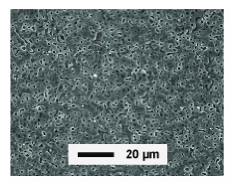
Figure 1: Electron microscopy image of a $c$-axis oriented HgBa₂CaCu₂O₆ thin film on SrTiO₃ substrate. Dense and homogeneous layers without irregular surface structures are fabricated under optimized conditions.

Figure 1 shows the surface of Hg-1212 layers that were produced from mercury-doped precursor films deposited at $T_{S}=350$ °C. The annealed films reveal a dense and homogeneous structure and smooth surface without $a$-axis oriented grains and regions of non-reacted material. The angular spread of the lattice axes orientation is less than 1° as measured by x-ray diffraction (rocking curves). For Hall measurements, two Hg-1212 films were patterned by standard photolithography and wet-chemical etching. The thickness of films was about 500 nm as measured by atomic force microscopy and the critical temperature was $T_{c0}\approx 120$ K.

The experimental setup for the electric transport measurements is made up of a closed-cycle refrigerator and an electromagnet. DC currents were injected in both directions and the polarity of the magnetic field was reversed multiple times for every data point to cancel spurious thermoelectric signals. The longitudinal and transverse voltages were measured simultaneously. Multiple data were taken by a Keithley 2182 nanovoltmeter and averaged at discrete temperature values, with a stability better than $\pm$ 0.01 K. The angle $\theta$ between the magnetic field $B$ and the in-plane current density $j_{x}$ was changed by rotating the electromagnet for every set of data. The sample was mounted between the electromagnet’s pole pieces in such way that a standard Hall measurement corresponds to $\theta=90\textdegree$. On the other hand at $\theta=0\textdegree$ $B$ is parallel to the current and to the $ab$-planes of the sample. For all in-field measurements a magnetic field of $B=1.13$ T was applied. The Hall voltage $V_{y}$ was measured at fixed position on adjacent side arms of the strip-shaped sample.

III results and comparison with theory

Figure 2 shows the temperature dependence of the longitudinal resistivity for the sample which had a slightly lower resistivity, as the magnetic field $B=1.13$ T is rotated in the plane determined by the $c$-axis and the current direction, at an angle $\theta$ with the latter. The results for the second sample are quite similar and are not shown here. The effect of an increasing $\theta$ at constant magnetic field, namely the broadening of the superconducting transition and the resistivity enhancement, is qualitatively similar to that of an increasing magnetic field applied orthogonally to the layers, as presented for instance in Ref. Puica et al., 2004. The difference between the effect of a perpendicular field $B_{z}$ compared to that of a tilted one with the same normal component $B_{z}=Bsin\theta$ becomes however evident at small angles, when $B$ is almost parallel to the layers. As one can see in Fig. 2, the zero-field curve (dotted) is clearly different from the one corresponding to $B=1.13$ T at $\theta=0$, where $B_{z}=0$. This fact points to the three-dimensional conduction character in the Hg-Ba-Ca-Cu-O compound, since for a pure two-dimensional in-plane conduction only the perpendicular-to-surface component is relevant.Larkin and Varlamov (2005)

Figure 2: Resistivity vs. temperature for different orientations of a magnetic field of fixed magnitude (solid curves). The arrow indicates the curve sequence corresponding to the increasing angle $\theta$ of the magnetic field with respect to the $ab$-plane (as well as to the current direction). The dotted curve shows the zero-field resistivity.

The measured Hall resistivity $\rho_{yx}=E_{y}/j_{x}$, where $E_{y}$ is the electric field between the adjacent side arms of the sample, is shown in Fig. 3. All the curves, except that for $\theta=0^{\circ}$, where no Hall signal could be detected, exhibit the change from the positive, hole-like sign in the normal state to the negative, electron-like one in the vortex-liquid regime, in accordance with previous investigations performed in the similar magnetic field range on other cuprates, like BSCCO-2223 (Ref. Lang et al., 1995) and YBCO (Ref. Puica et al., 2004). Furthermore, the second sign reversal, that is the subsequent return of the Hall resistivity to the positive value before vanishing, is also noticeable for the perpendicular orientation of the magnetic field (i.e. for $\theta=90^{\circ}$), as has been also previously observed in this compound,Kang et al. (1997) but is not discernable anymore at oblique orientations (see the inset in Figs. 3). This fact agrees with a similar observation on YBCO in Ref. Göb et al., 2000, where it was found that the second sign change disappeared in high current densities or under slightly tilted field direction, revealing thus its vortex pinning origin.

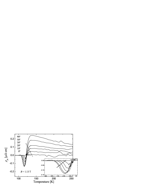
Figure 3: Hall resistivity $\rho_{yx}$ for the same sample and experimental conditions as in Fig. 2. The arrows indicates the curve sequence corresponding to the increasing angle $\theta$.

As well as for the longitudinal resistivity, one can notice that, qualitatively, the Hall resistivity behaves at increasing $\theta$ angle in the same manner as in increasing perpendicular-to-layers magnetic field $B_{z}$. To explore this situation, the Hall resistivity normalized to a constant magnetic field component perpendicular to the $ab$ plane, $B_{z}$, is shown in Fig. 4. Namely, the temperature of the positive-to-negative sign change shifts to lower values, the negative maximum of the Hall resistivity normalized to the out-of-plane component of the applied field becomes less sharp and decreases in magnitude, as observed for instance also in other cuprates.Puica et al. (2004) This behavior points to the fact that the effect of the magnetic field is mainly due to its out-of-plane component $B_{z}$. A good scaling of the Hall resistivity in the normal state can be observed, except for $\theta=10\textdegree$, where the large normalization factor introduces a considerable error.

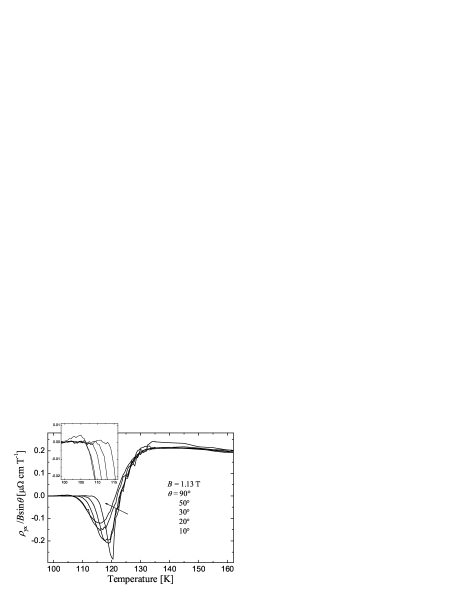
Figure 4: Hall resistivity $\rho_{yx}$ normalized to the out-of-plane field component $B\sin\theta$. The arrow shows the direction of the increasing angle $\theta$. The region of the second sign change is detailed in the inset.

However, more appropriate for a quantitative evaluation and comparison with a theoretical model for the Hall effect is to represent the Hall conductivity $\sigma_{xy}=\rho_{yx}/\left(\rho_{xx}^{2}+\rho_{yx}^{2}\right)$ as a function of temperature, as in Fig. 5, where $\sigma_{xy}$ is shown normalized to $B\sin\theta$. In this picture, it is easier to discern the delicate interplay of mainly three contributions to the Hall conductivity:Puica et al. (2004) (i) the positive quasiparticle vortex-core contribution, associated with normal-state excitations; (ii) superconducting contribution (excess Hall effect), resulting from the vortex flux-flow and superconducting fluctuations, which, by its negative sign, is essential to the occurrence of the first sign change; and (iii) pinning contribution which can eventually lead to the second sign reversal of the Hall effect. Theoretical calculations,Kopnin and Vinokur (1999) based on a simple model of pinning potential, suggested that an increasing pinning strength not only affects the longitudinal flux-flow resistivity, but also decreased the magnitude of the vortex contribution to the Hall voltage (fluctuation term in the Ginzburg-Landau approach). Strong enough pinning can thus result in a second sign reversal of the Hall resistivity, if the negative vortex (fluctuation) contribution is reduced in absolute value to magnitudes that are insufficient to counteract the positive contribution of the normal state conduction.Kopnin and Vinokur (1999); Ikeda (1999)

We shall try to give a quantitative account for the Hall conductivity data in Fig. 5 (symbols) for the temperature region corresponding to the first sign change and the negative maximum of $\rho_{yx}$, by considering the normal state contribution $\sigma_{xy}^{\mathrm{n}}$ and the superconducting fluctuation one $\Delta\sigma_{xy}$, such as

$$\sigma_{xy}=\sigma_{xy}^{\mathrm{n}}+\Delta\sigma_{xy}\,.$$ (1)

For the normal state part, we assume as valid Anderson’s formula:Anderson (1991) $\cot\theta_{H}^{\mathrm{n}}=\sigma_{xx}^{\mathrm{n}}/\sigma_{xy}^{\mathrm{n}}=C_{1}T^{2}+C_{0}$. We shall assume also a linear temperature dependence of the longitudinal resistivity in the normal state, so that the normal-state part of the conductivity tensor consists of the simple expressions:

$$\sigma_{xx}^{\mathrm{n}}=\frac{1}{p_{0}+p_{1}T}\>\>\>\text{and}\>\>\>\sigma_{xy}^{\mathrm{n}}=\frac{1}{p_{0}+p_{1}T}\cdot\frac{1}{C_{1}T^{2}+C_{0}}\>,$$ (2)

where $p_{0}$, $p_{1}$, $C_{1}$ and $C_{0}$ are to be determined from fits to the experiment.

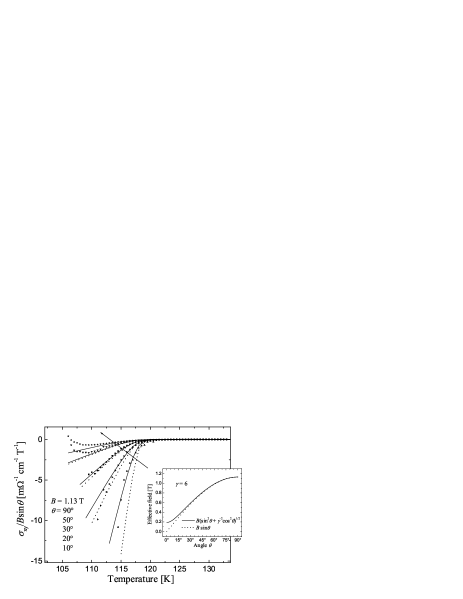
Figure 5: Experimental (symbols) and theoretical (curves) normalized Hall conductivity $\sigma_{xy}/B\sin\theta$ as a function of temperature. The arrow indicates the data sequence as $\theta$ increases. The solid curves represent the theoretical fits based on the rescaled field value $\widetilde{B}$, while for the dotted curves only the normal component $B\sin\theta$ is considered relevant. In the inset, the rescaled effective field $\widetilde{B}$ is compared to the out-of-plane field component $B_{z}=B\sin\theta$.

The fluctuation Hall conductivity $\Delta\sigma_{xy}$ was first theoretically calculated by Fukuyama, Ebisawa and Tsuzuki,Fukuyama et al. (1971) who pointed out that the origin of a non-vanishing Hall current due to fluctuating Cooper pairs could come from a particle-hole asymmetry, which reveals a complex relaxation time in the time dependent Ginzburg-Landau (TDGL) theory. In this early work, it was implicitly assumed that the fluctuations did not interact; that is, only Gaussian fluctuation were considered. Accordingly, the fluctuation parts of the conductivity tensor elements were predicted to diverge at $T_{c}$ in the presence of magnetic field. However, this predicted divergence has not been observed. A great improvement was obtained when the interaction between fluctuations was taken into account by incorporating the quartic term $\left|\psi\right|^{4}$ from the Ginzburg-Landau (GL) expression of the free energy. Such a treatment was performed by Ullah and DorseyUllah and Dorsey (1991) (UD) in the frame of a simple Hartree approach of the TDGL theory, while Nishio and EbisawaNishio and Ebisawa (1997) extended the calculations of the weak (Gaussian) fluctuation contribution of the Hall conductivity from Ref. Fukuyama et al., 1971 to the strong (non-Gaussian) fluctuation regime, based on more sophisticated renormalization theory by Ikeda, Ohmi and Tsuneto.Ikeda et al. (1991) The renormalized, non-Gaussian fluctuation regime connects therefore the weak (Gaussian) fluctuation regime in the paraconducting region above $T_{c}\left(H\right)$ to the vortex liquid (flux-flow) regime below the mean-field transition, interpolating smoothly without the $T_{c}$ divergence predicted by the Gaussian theory.

Due to its simpler form, we shall use in this paper the fluctuation Hall conductivity expression provided by the UD model,

$$\Delta\sigma_{xy}=-\alpha\frac{k_{B}T}{\varepsilon_{F}}\cdot\frac{e^{2}h^{3}}{2\hbar s}\int_{-\pi}^{\pi}\frac{dq}{2\pi}\sum_{n=0}^{N_{c}-1}\frac{n+1}{\widetilde{\varepsilon}_{nq}\widetilde{\varepsilon}_{n+1,q}\widetilde{\varepsilon}_{n+\frac{1}{2},q}^{2}}\,,$$ (3)

where $s$ is the distance between superconducting planes in the layered model, $h=B/B_{c2}(0)=2\xi_{0}^{2}eB/\hbar$ is the reduced magnetic field, supposed perpendicular to the layers, and $\widetilde{\varepsilon}_{nq}=\widetilde{\varepsilon}+\left(r/2\right)\left(1-\cos q\right)+\left(2n+1\right)h$, with $r=\left(2\xi_{0c}/s\right)^{2}$, while $\xi_{0}$ and $\xi_{0c}$ are the in-plane and, respectively, out-of-plane coherence lengths extrapolated at $T=0$. The value of $\alpha$, called the particle-hole asymmetry parameter,Fukuyama et al. (1971) can be inferred from the microscopical theory if one considers the energy derivative $\mathcal{N}^{\prime}$ of the density of states $\mathcal{N}$ at the Fermi level $\varepsilon_{F}$, and amounts in the BCS model to $\alpha=4\varepsilon_{F}\mathcal{N}^{\prime}/\pi g_{\mathrm{BCS}}\mathcal{N}^{2}$, with $g_{\mathrm{BCS}}$ ($>0$) the BCS coupling constant.Fukuyama et al. (1971); Nishio and Ebisawa (1997) The renormalized reduced temperature $\widetilde{\varepsilon}$ is calculated by solving the Hartree renormalization equation:Ullah and Dorsey (1991)

$$\widetilde{\varepsilon}-\ln\frac{T}{T_{0}} = 2gTh$$

$$\cdot\sum_{n=0}^{N_{c}}\frac{1}{\sqrt{\left(\widetilde{\varepsilon}+h+2nh\right)\left(\widetilde{\varepsilon}+h+2nh+r\right)}}\,,$$

where $g=2\mu_{0}\kappa_{\mathrm{GL}}^{2}e^{2}\xi_{0}^{2}k_{B}/\left(\pi\hbar^{2}s\right)$, with $\kappa_{\mathrm{GL}}$ being the in-plane Ginzburg-Landau parameter $\kappa_{\mathrm{GL}}=\lambda_{0}/\xi_{0}$, and $T_{0}$ is the mean-field transition temperature. The relationship between $T_{0}$ and $T_{c0}$, the actual renormalized critical temperature in zero-field, will be found by putting $\widetilde{\varepsilon}=0$ in Eq. (III) after taking the limit $B\rightarrow 0$ and it writes:Puica and Lang (2004)

$$T_{0}=T_{c0}\left[\sqrt{c/r}+\sqrt{1+(c/r)}\right]^{2gT_{c0}}\,.$$ (5)

The sums over the Landau levels (LL) in Eqs. (3) and (III) must be cut-off at some index $N_{c}$, reflecting the inherent UV divergence of the Ginzburg-Landau theory. This procedure suppresses the short wavelength fluctuating modes through a momentum (or, equivalently, kinetic energy) cut-off condition, which, in terms of the LL representation writes Ullah and Dorsey (1991); Mishonov and Penev (2000) $\hbar eB\left(2n+1\right)\leq c\hbar^{2}/2\xi_{0}^{2}$, with the cut-off parameter $c$ of the order of unity.

As already mentioned, the above model assumes a magnetic field perpendicular to the superconducting layers. The more general case with a magnetic field directed at some arbitrary angle $\theta$ with the $ab$-plane leads to the appearance of a vector potential in the $c$ direction, and the problem requires nontrivial calculations.Larkin and Varlamov (2005) In the close vicinity of the transition, however, where the out-of-plane coherence length grows much larger than the interlayer distance so that the details of the layered structure are no more relevant, the anisotropic three-dimensional (3D) fluctuation regime takes place. In the linear response approximation, i.e. for vanishing electric fields, even for an arbitrary orientation of the magnetic field, the transport coefficients in the anisotropic 3D model can be easily treated by using a special scaling transformation of the coordinates and field components in the GL equation.Blatter et al. (1992); Larkin and Varlamov (2005) This procedure reduces the problem to the isotropic case, where the coordinate system can be in turn freely rotated so that the magnetic field acquires again only one non-zero component.

Our experimental data correspond to the case when the magnetic field $B$ is applied in the $xz$-plane, at an angle $\theta$ with the $x$-axis, which represents the direction of the in-plane current density $j_{x}$. Following the results from Ref. Larkin and Varlamov, 2005, p. 68, we can directly write the Hall conductivity under the tilted field with the aid of the Hall conductivity under a rescaled field $\widetilde{B}$ applied along the $c$-direction:

$$\sigma_{xy}\left(\theta,B\right)=\sin\widetilde{\theta}\cdot\sigma_{xy}\left(0,\widetilde{B}\right)\,,$$ (6)

where

$$\widetilde{B} = B\sqrt{\sin^{2}\theta+\frac{1}{\gamma^{2}}\cos^{2}\theta}\,,$$

$$\tan\widetilde{\theta} = \gamma\tan\theta\,,$$ (7)

$$\gamma = \frac{\xi_{0}}{\xi_{0c}}\,.$$

Relation (6) can be transformed to

$$\frac{\sigma_{xy}\left(\theta,B\right)}{B\sin\theta}=\frac{\sigma_{xy}\left(0,\widetilde{B}\right)}{\widetilde{B}}\,,$$ (8)

which suggests that the experimental data (symbols) in Fig. 5 are to be compared with the theoretical results given by Eqs. (1-3) for the normalized Hall conductivity, provided the rescaled magnitude $\widetilde{B}$ of the magnetic field is considered. Such calculations are illustrated by the solid lines in Fig. 5, for which the following parameters, typical for the HgBa₂CaCu₂O₆ compound were used: $T_{c0}=118.2$ K, $\xi_{0}=1.5$ nm, $\xi_{0c}=0.25$ nm, $s=1.27$ nm, $\kappa_{\mathrm{GL}}=100$, $\varepsilon_{F}=1000$ K (in $k_{B}$ units).Kim et al. (1996); Puzniak (1994) The best fits were obtained for a particle-hole asymmetry parameter $\alpha=0.26$, which is comparable with the analogous value found from a similar fit Lang et al. (1995) for BSCCO-2223. The dotted curves in Fig. 5 show on the other hand the calculations with the same parameters, if only the out-of-plane component $B_{z}=B\sin\theta$ were taken into account instead of the rescaled value $\widetilde{B}$. One can notice that the two approaches give almost similar results at higher angles, where the rescaled magnitude $\widetilde{B}$ is almost identical with the normal component $B\sin\theta$, as illustrated in the inset of Fig. 5, but differ significantly for small angle $\theta$, when the field direction is close to the $ab$-plane and the difference between $\widetilde{B}$ and $B\sin\theta$ increases. The good quantitative agreement between the experimental data and the theoretical fits performed with the rescaled magnetic field values (solid curves) points therefore to the fluctuation origin of the Hall effect behavior in the temperature range corresponding to the first sign-change and the negative maximum of the Hall resistivity, as well as to the three-dimensional conduction character in the Hg-Ba-Ca-Cu-O compound.

IV Conclusions

In summary, we have investigated the resistivity of and the Hall effect in HgBa₂CaCu₂O₆ thin films when the magnetic field of fixed magnitude is rotated in the plane determined by the $c$-axis and the electric current direction. At first sight our measurements indicate qualitative similarity with the behavior in a variable magnetic field applied perpendicularly to the film, whose magnitude would be given by the out-of-plane component of the oblique field. This is also suggested by the rather good scaling of the Hall resistivity in the normal state with the out-of-plane magnetic field component (Fig. 4). However, the difference between the effect of a perpendicular field compared to that of a tilted one having the same normal component is revealed as the magnetic field approaches the orientation parallel to the layers, and is seen in both the resistivity (Fig. 2) and the Hall conductivity (Fig. 5) measurements. The second sign-change of the Hall angle in the lower part of the transition is found to disappear under oblique fields, pointing thus to its vortex pinning origin (inset in Fig. 4). The good quantitative agreement between the measured Hall conductivity and the theoretical fits based on the renormalized superconducting fluctuation model (Fig. 5), adapted through the field rescaling procedure in order to take into account the arbitrary orientation of the magnetic field, brings evidence for the anisotropic three-dimensional conduction character in the Hg-Ba-Ca-Cu-O compound close to $T_{c}$, as well as for the fluctuation origin of the Hall effect behavior in the vortex liquid region.