Influence of bound and unbound electron-hole-pair populations on the excitonic luminescence in semiconductor quantum wells

Abstract

A fully microscopic theory for the spontaneous emission from semiconductors is discussed. The theory is evaluated for a quantum-well system and the role of excitonic and unbound electron-hole-pair contributions to the emission is analyzed. Simplifying aproximations to the full theory and their range of validity are discussed. Numerical solutions are presented for experimentally relevant situations and it is shown that a detailed analysis of measured spectra requires the knowledge of both absorption and emission under identical conditions.

I Introduction

In this paper, we present a fully quantum mechanical analysis of spontaneous light emission from a Coulomb interacting carrier system in a semiconductor quantum well (QW). We are particularly interested to analyze the influence of excitonic and of unbound electron-hole-pair populations on the photo luminescence (PL) emitted at the spectral position of the exciton resonances.

Extensive experimental research in the past few decades has shown that one observes excitonic resonances in the PL of a QW for different material systems and for a very broad range of excitation conditions ranging from cryogenic (about 4 K) all the way to room temperatures.Stanley et al. (1991); Leroux et al. (1999) A PL resonance at the lowest $1s$-exciton state has also been observed even when the exciton ionizaton density is exceeded. For example, experiments with GaAs-type QW systems at 4 K lattice temperature show a clear excitonic resonance at the $1s$ position for a density range $10^{8}{\rm cm}^{-2}$ to $5\times 10^{10}{\rm cm}^{-2}$Khitrova et al. (1999); here, the lower density is only limited by the sensitivity in detection while the upper value is already beyond the ionization density.

The build-up of excitonic PL is often investigated in a configuration where the semiconductor is excited nonresonantly using ultrafast laser pulses that generate carriers into the high-energy states of the bands. Thus, all coherences vanish almost instantaneously and the direct generation of $1s$ excitons can be excluded. Using this scheme, it has been observedKumar et al. (1996); Hayes and Deveaud (2002) that an excitonic $1s$ PL resonance builds up on a subpicosecond timescale. Furthermore, excitonic PL is observed longer than several nanoseconds, which also implies that electron-hole pairs exist in the system for a very long time.

In order to explain some of the observe phenomena, Ref. Kira et al. (1998) developed a simple microscopic model for the semiconductor PL showing that also an electron-hole plasma, i.e. a system with nonvanishing electron and hole densities but no excitons, can produce PL spectra that peak at the exciton resonances. This prediction releases the previously assumed strict relation between the existence of exciton populations and the appearance of excitonic PL such that one can explain why excitonic PL is also observed under conditions where the presence of real exciton populations seems unreasonable.

In order to present a more complete analysis, we show in this paper how one can analyze self-consistently the electron-hole plasma and exciton-population effects in the QW PL. We show that in order to perform a reliable analysis, one has to evaluate not only the PL but also the corresponding absorption spectra recorded under equivalent conditions. Ideally, one should also measure the induced terahertz (THz) responseTimusk et al. (1978); Groeneveld and Grischkowsky (1994); Cerne et al. (1996); Kira et al. (2001); Kaindl et al. (2003); Galbraith et al. (2005).

Based on our microscopic analysis, we determine criteria under which exciton population effects are observed and when electron-hole plasma contributions are dominant. We also discuss the Coulomb-induced nonlinearities observable in PL for elevated densities. For this purpose, one clearly has to perform a quantitative analysis where the microscopic scattering, electron-hole plasma, and possible exciton populations have to be included microscopically. The developed analysis allows us to determine systematic criteria for a measured combination of absorption and PL to judge how much of a given PL spectrum can be attributed to excitonic and/or electron-hole plasma emission.

The discussion in this paper is organized as follows. We first present our general quantum theory for PL from coexisting electron-hole plasma end exciton populations. We show how this approach, with microscopic Coulomb scattering, can be formulated to compute the PL from quasi-stationary semiconductor populations consisting of a given exciton and electron-hole plasma population. We evaluate our theory numerically for a two-band QW model and present a detailed analysis of the exciton and electron-hole-plasma contibutions to the luminescence. We discuss different levels of simplifying approximations and emphasize the importance of the frequency and density dependent scattering. Finally, we summarize our results and use them to analyze experimental data. In the Appendices, we present technical details regarding the microscopic description of excitons and the density and frequency dependent scattering calculations.

II Microscopic theory of excitonic luminescence

We formulate our microscopic theory for the incoherent emission of a planar quantum well. In our calculations, we concentrate on PL resulting from recombinations involving only two bands, i.e. the energetically lowest conduction and the heavy-hole band. Multi-band effects can in principle be included in the theory, but they complicate the notation and do not contribute to the essence of our analysis. In the numerical evaluations, we use typical GaAs QW material parameters and choose the QW confinement such that the $2s$ resonance is 6 meV above the $1s$ state as observed in recent experiments.Chatterjee et al. (2004); Szczytko et al. (2004); Hoyer et al. (2005a); Szczytko et al. (2005) For semiconductors, the microscopic description of carrier excitations can be obtained with the help of the fermionic operators $a_{c,{\bf k}_{\|}}$ and $a^{\dagger}_{c,{\bf k}_{\|}}$ for conduction-band electrons and $a_{v,{\bf k}_{\|}}$ and $a^{\dagger}_{v,{\bf k}_{\|}}$ for valence-band electrons having momentum ${\bf k}_{\|}$ in the QW plane. The quantized light field is described by bosonic operators $B_{{\bf q}_{\|},q_{\perp}}$ and $B^{\dagger}_{{\bf q}_{\|},q_{\perp}}$ related to free space eigen modes with momentum ${\bf q}=({\bf q}_{\|},q_{\perp})$ that is divided into the ${\bf q}_{\|}$ component in the QW plane and $q_{\perp}$ perpendicular to the QW. The full system Hamiltonian of the interacting carrier-photon system is discussed e.g. in Refs. Haug and Koch, 2004; Kira et al., 1999 and the relating microscopic PL dynamics is derived in Refs. Kira et al., 1997a, 1998, 1999, 2001; Hoyer et al., 2003; Kira and Koch, 2005, 2006. Here, we therfore present only a brief summary of the elements important for our analysis of excitonic PL.

Since we want to compute PL from incoherent quasiparticle excitations, we concentrate on conditions where the coherent polarization and the coherent fields $\langle B_{\bf q}\rangle$ vanish. We also assume that the system is homogeneously excited and quasi stationary. For such conditions, the single-particle distributions

$$f^{e}_{{\bf k}_{\|}}\equiv\langle a^{\dagger}_{c,{\bf k}_{\|},c}a_{c,{\bf k}_{\|}}\rangle,\;\;\;\;f^{h}_{{\bf k}_{\|}}\equiv\langle a_{v,{\bf k}_{\|}}a^{\dagger}_{v,{\bf k}_{\|}}\rangle,$$ (1)

for the electrons and holes can be taken as constant.

The relevant two-particle correlations in the incoherent regime are excitonic and pure intraband carrier correlations.Kira et al. (2001); Hoyer et al. (2003) For the study of PL, we only need to evaluate the excitonic correlations defined as

$$c_{X}^{{\bf q}_{\|},{\bf k}^{\prime}_{\|},{\bf k}_{\|}}\equiv\Delta\langle a^{\dagger}_{c,{\bf k}_{\|}}a^{\dagger}_{v,{\bf k}^{\prime}_{\|}}a_{c,{\bf k}^{\prime}_{\|}+{\bf q}_{\|}}a_{v,{\bf k}_{\|}-{\bf q}_{\|}}\rangle$$

$$\;\;\;\;\;\;\;\;\;\;=\langle a^{\dagger}_{c,{\bf k}_{\|}}a^{\dagger}_{v,{\bf k}^{\prime}_{\|}}a_{c,{\bf k}^{\prime}_{\|}+{\bf q}_{\|}}a_{v,{\bf k}_{\|}-{\bf q}_{\|}}\rangle-\langle a^{\dagger}_{c,{\bf k}_{\|}}a^{\dagger}_{v,{\bf k}^{\prime}_{\|}}a_{c,{\bf k}^{\prime}_{\|}+{\bf q}_{\|}}a_{v,{\bf k}_{\|}-{\bf q}_{\|}}\rangle_{\rm S},$$ (2)

where the subtracted single-particle contribution $\langle a^{\dagger}_{\lambda}a^{\dagger}_{\nu}a_{\nu^{\prime}}a_{\lambda^{\prime}}\rangle_{\rm S}$ is obtained by using the usual Hartree-Fock approximation $\langle a^{\dagger}_{\lambda}a^{\dagger}_{\nu}a_{\nu^{\prime}}a_{\lambda^{\prime}}\rangle_{\rm S}\equiv\langle a^{\dagger}_{\lambda}a_{\lambda^{\prime}}\rangle\langle a^{\dagger}_{\nu}a_{\nu^{\prime}}\rangle-\langle a^{\dagger}_{\lambda}a_{\nu^{\prime}}\rangle\langle a^{\dagger}_{\nu}a_{\lambda^{\prime}}\rangle$.

The incoherent photon correlations and the microsocpic source for the PL are obtained from the photon-assisted electron-hole recombination and the photon-number-like correlations

$$\Pi_{{\bf k}_{\|},{\bf q}_{\|},q_{\perp}}\equiv\Delta\langle B^{\dagger}_{{\bf q}_{\|},q_{\perp}}a_{v,{\bf k}_{\|}}^{\dagger}a_{c,{\bf k}_{\|}+{\bf q}_{\|}}\rangle$$

$$\;\;\;\;\;\;\;\;\;\;=\langle B^{\dagger}_{{\bf q}_{\|},q_{\perp}}a_{v,{\bf k}_{\|}}^{\dagger}a_{c,{\bf k}_{\|}+{\bf q}_{\|}}\rangle-\langle B^{\dagger}_{{\bf q}_{\|},q_{\perp}}\rangle\langle a_{v,{\bf k}_{\|}}^{\dagger}a_{c,{\bf k}_{\|}+{\bf q}_{\|}}\rangle,$$

$$\Delta\langle B^{\dagger}_{{\bf q}_{\|},q_{\perp}}B_{{\bf q}_{\|},q^{\prime}_{\perp}}\rangle\equiv\langle B^{\dagger}_{{\bf q}_{\|},q_{\perp}}B_{{\bf q}_{\|},q^{\prime}_{\perp}}\rangle-\langle B^{\dagger}_{{\bf q}_{\|},q_{\perp}}\rangle\langle B_{{\bf q}_{\|},q^{\prime}_{\perp}}\rangle,$$ (3)

respectively. These are obtained by subtracting the classical factorizations from the full expectation values. Once these quantities are determined microscopically, we can evaluate the semiconductor PL and study the influence of electron-hole plasma and exciton populations.

The exciton correlation dynamics follows from

$$i\hbar\frac{\partial}{\partial t}c^{{\bf q}_{\|},{\bf k}^{\prime}_{\|},{\bf k}_{\|}}_{\rm X} = \epsilon^{{\bf q}_{\|},{\bf k}^{\prime}_{\|},{\bf k}_{\|}}c^{{\bf q}_{\|},{\bf k}^{\prime}_{\|},{\bf k}_{\|}}_{\rm X}+S^{{\bf q}_{\|},{\bf k}^{\prime}_{\|},{\bf k}_{\|}}$$ (4)

$$+ \left(1-f^{e}_{{\bf k}_{\|}}-f^{h}_{{\bf k}_{\|}-{\bf q}_{\|}}\right)\sum_{{\bf l}_{\|}}V_{{\bf l}_{\|}-{\bf k}_{\|}}c^{{\bf q}_{\|},{\bf k}^{\prime}_{\|},{\bf l}_{\|}}_{\rm X}-\left(1-f^{e}_{{\bf k}^{\prime}_{\|}+{\bf q}_{\|}}-f^{h}_{{\bf k}^{\prime}_{\|}}\right)\sum_{{\bf l}_{\|}}V_{{\bf l}_{\|}-{\bf k}^{\prime}_{\|}}c^{{\bf q}_{\|},{\bf l}_{\|},{\bf k}_{\|}}_{\rm X}$$

$$- i(1-f^{e}_{{\bf{k}}_{\|}}-f^{h}_{{\bf{k}}_{\|}-{\bf{q}}_{\|}})\Pi_{{\bf k}^{\prime}_{\|},{\bf q}_{\|},\Sigma}-i(1-f^{e}_{{\bf{k}}^{\prime}_{\|}-{\bf{q}}_{\|}}-f^{h}_{{\bf{k}}^{\prime}_{\|}})\Pi^{\star}_{{\bf k}_{\|}-{\bf q}_{\|},{\bf q}_{\|},\Sigma}$$

$$+ D^{{\bf q}_{\|},{\bf k}^{\prime}_{\|},{\bf k}_{\|}}_{\rm rest}-iT^{{\bf q}_{\|},{\bf k}^{\prime}_{\|},{\bf k}_{\|}},$$

where we have introduced the renormalized electron-hole pair energy

$$\epsilon^{{\bf q}_{\|},{\bf k}^{\prime}_{\|},{\bf k}_{\|}}\equiv\epsilon^{c}_{{\bf k}_{\|}-{\bf q}_{\|}}-\epsilon^{v}_{{\bf k}_{\|}}-\epsilon^{c}_{{\bf k}^{\prime}_{\|}}+\epsilon^{v}_{{\bf k}^{\prime}_{\|}+{\bf q}_{\|}}-\sum_{\bf l}V_{{\bf l}_{\|}}\left[f^{e}_{{\bf k}_{\|}-{\bf q}_{\|}-{\bf l}_{\|}}+f^{h}_{{\bf k}_{\|}-{\bf l}_{\|}}-f^{e}_{{\bf k}^{\prime}_{\|}-{\bf l}_{\|}}-f^{h}_{{\bf k}^{\prime}_{\|}+{\bf q}_{\|}-{\bf l}_{\|}}\right].$$ (5)

Furthermore, we have defined a collective photon assisted electron-hole recombination term

$$\Pi_{{\bf k}_{\|},{\bf q}_{\|},\Sigma}\equiv\Delta\langle B^{\dagger}_{{\bf q}_{\|},\Sigma}a_{v,{\bf k}_{\|}}^{\dagger}a_{c,{\bf k}_{\|}+{\bf q}_{\|}}\rangle,$$ (6)

$$B_{{\bf q}_{\|},\Sigma}\equiv\sum_{q_{\perp}}{\cal F}_{{\bf q},q_{\perp}}B_{{\bf q},q_{\perp}},$$ (7)

where ${\cal F}_{{\bf q}}\equiv d_{vc}\sqrt{\frac{\hbar\omega_{\bf q}}{2\epsilon_{0}}}u_{\bf q}$ determines the strength of the light-matter interaction via the dipole-matrix element $d_{vc}$ and the mode function $u_{\bf q}$ at the QW position. The square-root term is the so-called vacuum field amplitude containing the light frequency $\omega_{\bf q}$.

The single-particle source of Eq. (4) originates from the Coulomb interaction and has the explicit form

$$S^{{\bf q}_{\|},{\bf k}^{\prime}_{\|},{\bf k}_{\|}} = V_{{\bf k}^{\prime}_{\|}+{\bf q}_{\|}-{\bf k}_{\|}}\left[(1-f^{e}_{{\bf k}_{\|}})(1-f^{h}_{{\bf k}_{\|}-{\bf q}_{\|}})f^{e}_{{\bf k}^{\prime}_{\|}+{\bf q}_{\|}}f^{h}_{{\bf k}^{\prime}_{\|}}-f^{e}_{{\bf k}_{\|}}f^{h}_{{\bf k}_{\|}-{\bf q}_{\|}}(1-f^{e}_{{\bf k}^{\prime}_{\|}+{\bf q}_{\|}})(1-f^{h}_{{\bf k}^{\prime}_{\|}})\right].$$ (8)

This expression describes the Coulomb-induced scattering contributions which develop the electron-hole plasma into a correlated state even when no correlations are present initially.

Equation (4) also contains several Coulomb sums. Here, we have explicitly presented only those terms that contain the phase-space filling factor $(1-f^{e}-f^{h})$ since they describe the attractive interaction between electrons and holes allowing them to become truly bound electron-hole pairs, i.e. incoherent excitons. These Coulomb sums are referred to as the main-sum contributions.Hoyer et al. (2003) The other Coulomb sums, denoted symbolically as $D_{\rm rest}$, consist of terms of the form $(f^{\lambda}-f^{\nu})\sum V\;c$. Since $(f^{\lambda}-f^{\nu})$ is much smaller than $(1-f^{e}-f^{h})$ for low enough densities, $D_{\rm rest}$ has a much smaller effect on the exciton correlations than the main-sum terms for conditions where bound excitons still exist.Hoyer et al. (2003) Thus, we may apply the main-sum approximation where $D_{\rm rest}$ is omitted when we compute the excitonic PL. Besides the two-particle correlations, Eq. (4) also contains three-particle correlation terms symbolized by $T^{{\bf q},{\bf k}^{\prime},{\bf k}}$. The description of these terms is presented in Appendix B.

The incoherent carrier quantities enter as sources to the semiconductor luminescence equations Kira et al. (1997a, 1999, 2004); Kira and Koch (2005)

$$\frac{\partial}{\partial t}\Delta\langle B^{\dagger}_{{\bf q}_{\|},q_{\perp}}B_{{\bf q}_{\|},q^{\prime}_{\perp}}\rangle=i\left(\omega_{q}-\omega_{q^{\prime}}\right)\Delta\langle B^{\dagger}_{{\bf q}_{\|},q_{\perp}}B_{{\bf q}_{\|},q^{\prime}_{\perp}}\rangle+{\textstyle\sum_{{\bf k}}}\left[{\cal{F}}_{q}\Pi^{\star}_{{\bf k}_{\|},{\bf q}_{\|},q^{\prime}_{\perp}}+{\cal{F}}^{\star}_{q^{\prime}}\Pi_{{\bf k}_{\|},{\bf q}_{\|},q_{\perp}}\right]$$ (9)

$$\frac{\partial}{\partial t}\Pi_{{\bf k}_{\|},{\bf q}_{\|},q_{\perp}}=\frac{1}{i\hbar}\left[\left(\tilde{\epsilon}_{{\bf k}_{\|},{\bf q}_{\|}}-\hbar\omega_{\bf q}\right)\Pi_{{\bf k}_{\|},{\bf q}_{\|},q_{\perp}}-\left[1-f^{e}_{{\bf k}_{\|}+{\bf q}_{\|}}-f^{h}_{{\bf k}_{\|}}\right]\sum_{{\bf l}_{\|}}V_{{\bf k}_{\|}-{\bf l}_{\|}}\Pi_{{\bf l}_{\|},{\bf q}_{\|},q_{\perp}}\right]$$

$$+{\cal F}_{q}\left[f^{e}_{{\bf k}_{\|}+{\bf q}_{\|}}f^{h}_{{\bf k}_{\|}}+\sum_{{\bf l}_{\|}}c_{X}^{{\bf q}_{\|},{\bf k}_{\|},{\bf l}_{\|}}\right]-\left[1-f^{e}_{{\bf k}_{\|}+{\bf q}_{\|}}-f^{h}_{{\bf k}_{\|}}\right]\Delta\langle B^{\dagger}_{{\bf q}_{\|},q_{\perp}}B_{{\bf q}_{\|},\Sigma}\rangle-iT^{\Pi}_{{\bf k}_{\|},{\bf q}_{\|},q_{\perp}}.$$ (10)

Here,

$$\tilde{\epsilon}_{{\bf k}_{\|},{\bf q}_{\|}}=\epsilon^{c}_{{\bf k}_{\|}+{\bf q}_{\|}}-\epsilon^{v}_{{\bf k}_{\|}}-\sum_{{\bf l}_{\|}}V_{{\bf k}_{\|}-{\bf l}_{\|}}\left[f^{e}_{{\bf l}_{\|}+{\bf q}_{\|}}+f^{h}_{{\bf l}_{\|}}\right]$$ (11)

is the renormalized kinetic energy. The first term in the second line of Eq. (10) shows that photon-assisted recombination processes can be seeded either by an electron-hole plasma population ($f^{e}f^{h}$) or an exciton correlation term ($c_{X}$). Since these spontaneous emission sources do not depend on the photon frequency, both plasma and exciton correlation sources contribute to the PL in the same spectral range.

The second term in Eq. (10) shows that the photon-assisted recombination processes for different momentum combinations are coupled via the Coulomb interaction. This renormalization determines the emission frequency similar to the classical field renormalization in the semicondcutor Bloch equations Lindberg and Koch (1988); Haug and Koch (2004); Kira and Koch (2004, 2006). Since this Coulomb correlation effect is not at all related to the specific spontaneous emission source, even the existence of bare electron and hole densities leads to emission of light at the bound exciton frequencies. When the QW is not inside a cavity, the stimulated feedback term, $\Delta\langle B^{\dagger}B_{\Sigma}\rangle$, in Eq. (10) is negligible. The explicit form of the three-particle scattering term, $T^{\Pi}$, is discussed in Appendix B.

II.1 Excitons vs. correlated electron-hole plasma

As a very broad definition, an exciton is a quasi-particle that consist of a bound electron-hole pair. This interpretation is seemingly simple and straightforward. However, once one seriously considers the fact that an exciton has a fermionic substructure, as is done in Eq. (4), one realizes that one can neither define a pure exciton operator nor a rigorous number operator for excitons in a fermionic many-body system.Usui (1960) As a working definition, we speak of an exciton in a many-particle system if at least one electron depends on a hole in a correlated manner, where the correlation is in the relative motion coordinate. The pair wavefunction is determined from the Wannier equation that is analogous to the generalized Schrödinger equation for the hydrogen. The bound state solutions define the bound excitons while the ionized states define ionized excitons.

The Wannier equation in momentum space is equivalent to the Fourier transform of the Hydrogen equation, but can contain additional energy renormalizations and a phase-space filling factor if a finite amount of carriers is present.Haug and Koch (2004) As shown in Appendix A, it is even possible to incorporate carrier scattering in the Wannier equation and thus obtain excitonic quasi-particles including Coulomb scattering effects. In the presence of carriers, both the phase-space filling factor and the microscopic scattering make the corresponding eigenvalue problem non-Hermitian, such that a left-handed and a right-handed basis set ($\Phi_{\nu,{\bf{q}}_{\|}}^{L/R}$) must be introduced, see Appendix A. There, we show that the definition of true excitons can be mathematically formulated by using the transformations

$$\Delta N_{\lambda,\nu}({\bf q}_{\|}) = \sum_{{\bf k}_{\|},{\bf k}^{\prime}_{\|}}\Phi^{L}_{\lambda,{\bf{q}}_{\|}}({\bf k}_{\|})\left(\Phi^{L}_{\nu,{\bf{q}}_{\|}}({\bf k}^{\prime}_{\|})\right)^{\star}c^{{\bf q}_{\|},{\bf k}^{\prime}_{\|}-{\bf q}_{h},{\bf k}_{\|}+{\bf q}_{e}}_{\rm X},$$ (12)

$$c^{{\bf q}_{\|},{\bf k}^{\prime}_{\|},{\bf k}_{\|}}_{\rm X} = \sum_{\lambda,\nu}\left(\Phi^{R}_{\lambda,{\bf{q}}_{\|}}({\bf k}_{\|}-{\bf q}_{e})\right)^{\star}\Phi^{R}_{\nu,{\bf{q}}_{\|}}({\bf k}^{\prime}_{\|}+{\bf q}_{h})\Delta N_{\lambda,\nu}({\bf q}_{\|}),$$ (13)

where the excitonic center-of-mass momentum has been split symmetrically via

$${\bf q}_{e}=\frac{m_{e}}{m_{e}+m_{h}}{\bf q}_{\|},\;\;\;\;{\bf q}_{h}=\frac{m_{h}}{m_{e}+m_{h}}{\bf q}_{\|}.$$ (14)

In particular, the diagonal elements,

$$\Delta N_{\lambda}({\bf q}_{\|})\equiv\Delta N_{\lambda,\lambda}({\bf q}_{\|}),$$ (15)

define the momentum distribution for excitons in state $\lambda$.

The physical relevance of these quantities can be verified by analyzing THz absorption which is shownKira et al. (2001, 2004) to probe exclusively $\sum_{{\bf q}_{\|}}\Delta{N}_{\lambda}({\bf q}_{\|})$ under incoherent conditions. More precisely, each exciton state can be connected with a population

$$\Delta{n}_{\lambda}=\frac{1}{S}\sum_{{\bf q}_{\|}}\Delta{N}_{\lambda}({\bf q}_{\|})$$ (16)

and a $1s$-to-$2p$ resonance in the linear THz absorption shows unambiguously that the $1s$ state is initially populated. In full analogy to the optical transitions in atomic systems, the strength of the resonance is directly related to the population difference between the initial $\Delta n_{1s}$ and the final $\Delta n_{2p}$ states. Thus, THz spectroscopy shows that $\Delta n_{\beta}$ defines the exciton density of a given state in the same way as one can count atoms occupying different atomic states by using optical spectroscopy.

In general, exciton correlations can also exhibit nondiagonal $\lambda\neq\nu$ contributions in $\Delta N_{\lambda,\nu}$. As shown in Ref. Hoyer et al. (2003), these off-diagonal parts build up on a pico-second timescale and can be identified with a correlated plasma while the diagonal exciton populations are formed much more slowly. In the present publication we include microscopic Coulomb scattering beyond the constant dephasing and we include both diagonal and non-diagonal exciton correlations.

II.2 Incoherent quasiparticle states

As already argued in Chatterjee et al. (2004), it is essential to analyze the experimental PL together with absorption spectra obtained under identical conditions. Since many experiments measure PL in the normal direction, we consider this configuration here. Using our formalism, we establish a connection between the quasi-particle state and the measured spectra in order to determine the conditions and excitation parameters where excitonic populations significantly influence PL experiments.

When a weak classical optical pulse, $E(t)$, is applied to probe the incoherent excitation state of a semiconductor, it does not alter electron, hole, or exciton populations. The probe pulse interacts with the system, merely by inducing the optical (probe) polarization $P_{{\bf k}_{\|}}\equiv\langle a^{\dagger}_{v,{\bf k}_{\|}}a_{c,{\bf k}_{\|}}\rangle$ in the system. Thus, we need to solve the polarization dynamics from the semiconductor Bloch equations Lindberg and Koch (1988); Haug and Koch (2004)

$$i\hbar\frac{\partial}{\partial t}P_{{\bf k}_{\|}}=\tilde{\epsilon}_{{\bf k}_{\|}}P_{{\bf k}_{\|}}-\left[1-f^{e}_{{\bf k}_{\|}}-f^{h}_{{\bf k}_{\|}}\right]\sum_{{\bf k}^{\prime}_{\|}}V_{{\bf k}^{\prime}_{\|}-{\bf k}_{\|}}P_{{\bf k}^{\prime}_{\|}}$$

$$\;\;\;\;\;\;\;\;\;\;-\left[1-f^{e}_{{\bf k}_{\|}}-f^{h}_{{\bf k}_{\|}}\right]d_{c,v}E(t)-i\Gamma_{{\bf k}_{\|}}$$ (17)

which contains two-particle Coulomb- and phonon-induced scattering terms in $\Gamma_{{\bf k}_{\|}}$. Performing a Fourier transformation of Eq. (17), we obtain

$$(\hbar\omega-\tilde{\epsilon}_{{\bf k}_{\|}})P_{{\bf k}_{\|}}(\omega)=-\left[1-f^{e}_{{\bf k}_{\|}}-f^{h}_{{\bf k}_{\|}}\right]\sum_{{\bf k}^{\prime}_{\|}}V_{{\bf k}^{\prime}_{\|}-{\bf k}_{\|}}P_{{\bf k}^{\prime}_{\|}}(\omega)$$

$$\;\;\;\;\;\;\;\;\;\;-\left[1-f^{e}_{{\bf k}_{\|}}-f^{h}_{{\bf k}_{\|}}\right]d_{c,v}E(\omega)-i\Gamma_{{\bf k}_{\|}}(\omega),$$ (18)

where we describe the Coulomb-induced scattering

$$\Gamma_{{\bf k}_{\|}}(\omega)=\gamma^{{\mathrm{D}}}_{{\bf k}_{\|}}(\omega)P_{{\bf k}_{\|}}(\omega)-\sum_{{\bf k}^{\prime}_{\|}}\gamma^{{\mathrm{OD}}}_{{\bf k}_{\|},{\bf k}^{\prime}_{\|}}(\omega)P_{{\bf k}^{\prime}_{\|}}(\omega)$$ (19)

via the diagonal and off-diagonal excitation-induced dephasing matrices $\gamma^{{\mathrm{D}}}$ and $\gamma^{{\mathrm{OD}}}$. Their detailed form is given in Appendix B.

The linear absorption spectrum follows from

$$\alpha(\omega)\equiv{\rm Im}\left[\frac{1}{\epsilon_{0}{\cal S}}\sum_{{\bf k}_{\|}}\frac{d_{{\bf k}^{\prime}_{\|}}P_{{\bf k}^{\prime}_{\|}}(\omega)}{E(\omega)}\right].$$ (20)

If the semiconductor system is in thermodynamic equilibrium, the linear absorption, $\alpha(\omega)$ and PL spectrum, $PL(\omega)$ are connected viaZimmermann (1988) the well-known thermal relation

$$I_{PL}^{\rm TD}(\omega)\equiv\frac{\alpha(\omega)}{e^{(\hbar\omega-\mu)/(k_{B}T)}-1}$$ (21)

where $\omega$ is the angular frequency of the light, $\mu$ is the chemical potential of electron-hole pairs, and $T$ is the lattice temperature. For dilute densities, the Bose-Einstein distribution can be replaced by a Boltzmann distribution. Clearly, $I_{PL}^{\rm TD}(\omega)$ provides a well-defined reference point under all excitation conditions. In fact, the relative contribution of the electron-hole plasma to the excitonic PL can be identified by quantifying how strongly the actually measured PL deviates from the thermodynamic limit.

Under quasistationary conditions, the steady-state PL emitted in normal direction, ${\bf q}_{\|}=0$, is obtained from Eq. (9)–(10) as

$$I_{PL}(\omega=c|{\bf q}|)\equiv\frac{\partial}{\partial t}\Delta\langle B^{\dagger}_{0,q_{\perp}}B_{0,q_{\perp}}\rangle={\rm Re}\left[\sum_{{\bf k}_{\|}}{\cal{F}}^{\star}_{q^{\prime}}\Pi_{0,{\bf q}_{\|},q_{\perp}}\right]$$ (22)

$$\frac{\partial}{\partial t}\Pi_{{\bf k}_{\|},0,q_{\perp}}=\frac{1}{i\hbar}\left[\left(\tilde{\epsilon}_{{\bf k}_{\|},{\bf q}_{\|}}-\hbar\omega_{\bf q}\right)\Pi_{{\bf k}_{\|},0,q_{\perp}}-\left[1-f^{e}_{{\bf k}_{\|}}-f^{h}_{{\bf k}_{\|}}\right]\sum_{{\bf l}_{\|}}V_{{\bf k}_{\|}-{\bf l}_{\|}}\Pi_{{\bf l}_{\|},0,q_{\perp}}\right]$$

$$\;\;\;\;\;\;\;\;\;\;\;\;\;\;\;\;\;\;\;\;+{\cal F}_{q}\left[f^{e}_{{\bf k}_{\|}}f^{h}_{{\bf k}_{\|}}+\sum_{{\bf l}_{\|}}c_{X}^{0,{\bf k}_{\|},{\bf l}_{\|}}\right]-iT^{\Pi}_{{\bf k}_{\|},0,q_{\perp}}.$$ (23)

Here, we have omitted the stimulated contributions since they are insignificant for bare QW systems. As shown in App. B, the three-particle scattering terms can be cast into a form similar to the polarization scattering in Eq. (19), i.e.

$$T^{\Pi}_{{\bf k}_{\|},0,q_{\perp}}\equiv\gamma^{{\mathrm{D}}}_{{\bf k}_{\|}}(\omega_{q_{\perp}})\Pi_{{\bf k}_{\|},0,q_{\perp}}-\sum_{{\bf k}^{\prime}_{\|}}\gamma^{{\mathrm{OD}}}_{{\bf k}_{\|},{\bf k}^{\prime}_{\|}}(\omega)\Pi_{{\bf k}^{\prime}_{\|},0,q_{\perp}}.$$ (24)

Thus, the semiconductor Bloch and luminescence equations exhibit the same generic structure. However, as the major difference, the semiconductor PL has as its incoherent source the combination of carrier densities $f^{e}f^{h}$ and exciton correlations while the optical polarization is driven by the coherent field $E(\omega)$.

The incoherent quasi-particle correlations enter Eq. (23) via $c_{X}$. To separate the exciton-population and correlated electron-hole plasma contributions, we introduce

$$c^{0,{\bf k}^{\prime}_{\|},{\bf k}_{\|}}_{\rm X}=\sum_{\lambda}\left(\Phi^{R}_{\lambda,{\bf{q}}_{\|}}({\bf k}_{\|})\right)^{\star}\Phi^{R}_{\lambda,{\bf{q}}_{\|}}({\bf k}^{\prime}_{\|})\Delta N_{\lambda,\lambda}(0)+c^{0,{\bf k}^{\prime}_{\|},{\bf k}_{\|}}_{\rm plasma},$$ (25)

where the steady-state form of the correlated plasma part is obtained from Eq. (4)

$$i\hbar\frac{\partial}{\partial t}c^{0,{\bf k}^{\prime}_{\|},{\bf k}_{\|}}_{\rm plasma}=\epsilon^{0,{\bf k}^{\prime}_{\|},{\bf k}_{\|}}c^{0,{\bf k}^{\prime}_{\|},{\bf k}_{\|}}_{\rm X}$$

$$\;\;\;\;\;\;\;\;\;\;+V_{{\bf k}^{\prime}_{\|}-{\bf k}_{\|}}\left[(1-f^{e}_{{\bf k}_{\|}})(1-f^{h}_{{\bf k}_{\|}})f^{e}_{{\bf k}^{\prime}_{\|}}f^{h}_{{\bf k}^{\prime}_{\|}}-f^{e}_{{\bf k}_{\|}}f^{h}_{{\bf k}_{\|}}(1-f^{e}_{{\bf k}^{\prime}_{\|}})(1-f^{h}_{{\bf k}^{\prime}_{\|}})\right]$$

$$\;\;\;\;\;\;\;\;\;\;+\left(1-f^{e}_{{\bf k}_{\|}}-f^{h}_{{\bf k}_{\|}}\right)\sum_{{\bf l}_{\|}}V_{{\bf l}_{\|}-{\bf k}_{\|}}c^{0,{\bf k}^{\prime}_{\|},{\bf l}_{\|}}_{\rm plasma}-\left(1-f^{e}_{{\bf k}^{\prime}_{\|}}-f^{h}_{{\bf k}^{\prime}_{\|}}\right)\sum_{{\bf l}_{\|}}V_{{\bf l}_{\|}-{\bf k}^{\prime}_{\|}}c^{0,{\bf l}_{\|},{\bf k}_{\|}}_{\rm plasma}$$

$$\;\;\;\;\;\;\;\;\;\;-i\sum_{{\bf l}_{\|}}\left[\gamma^{X}_{{\bf k}_{\|},{\bf l}_{\|}}\right]^{\star}c^{0,{\bf k}^{\prime}_{\|},{\bf l}_{\|}}_{\rm plasma}-i\sum_{{\bf l}_{\|}}\gamma^{X}_{{\bf k}^{\prime}_{\|},{\bf l}_{\|}}c^{0,{\bf l}_{\|},{\bf k}_{\|}}_{\rm plasma}.$$ (26)

Here, the main-sum approximation has been made and the spontaneous recombination term is omitted since it mostly influences the exciton population. We have also presented the three-particle scattering terms induced by the Coulomb scattering via $\gamma^{X}_{{\bf k}_{\|},{\bf k}^{\prime}_{\|}}$.

The incoherent particle states are characterized by the respective single-particle carrier distributions $f^{e/h}$ and the exciton populations $\Delta{N}_{\lambda}$. Hence, under the assumed quasi-stationary conditions the PL can be solved for a given configuration by specifying $f^{e/h}$ and $\Delta{N}_{\lambda}$. For low densities, and if we assume that the scattering can be approximated by a simple dephasing constant $\gamma$, Eq. (26) reduces to

$$\Delta N_{\lambda,\nu}^{\rm plasma}({\bf q}_{\|}) = \frac{E_{\nu}-E_{\lambda}}{E_{\nu}-E_{\lambda}-i\gamma}\sum_{{\bf k}_{\|}}\Phi^{L}_{\lambda}({\bf k}_{\|})f^{e}_{{\bf k}_{\|}+{\bf q}_{e}}f^{h}_{{\bf k}_{\|}-{\bf q}_{h}}\Phi^{L}_{\nu}({\bf k}_{\|})$$ (27)

showing that this correlated plasma contribution does not contain densities since the diagonal terms $\nu=\lambda$ vanish.

II.3 Analytical approximations

To obtain an analytical understanding of the fully numerical solutions of the complete equations, it is beneficial to introduce a generalized exciton basis in order to diagonalize the homogeneous parts of Eqs. (18), (23) and (26). Since these equations include also carrier-carrier scattering, energy renormalizations and phase-space filling factors, a suitable exciton basis clearly must go beyond the usual low-density Wannier wavefunctions.

The basis set for solving Eqs. (18) and (23) is obtained from the solution of the generalized Wannier equation,

$$\sum_{{\bf k}^{\prime}_{\|}}\mathbf{M}_{{\bf{k}}_{\|},{\bf{k}}^{\prime}_{\|}}(\omega)\varphi^{R}_{\nu}({\bf k^{\prime}}_{\|},\omega)=(E_{\nu}(\omega)-i\Gamma_{\nu}(\omega))\varphi^{R}_{\nu}({\bf k}_{\|},\omega)$$ (28)

with the matrix $\mathbf{M}$ defined as

$$M_{{\bf{k}}_{\|},{\bf{k}}^{\prime}_{\|}}(\omega) = [\tilde{\epsilon}_{{\bf k}_{\|}}-i\gamma^{{\mathrm{D}}}_{{\bf{k}}_{\|}}(\omega)]\delta_{{\bf k}^{\prime}_{\|},{\bf k}_{\|}}-\left[1-f^{e}_{{\bf k}_{\|}}-f^{h}_{{\bf k}_{\|}}\right]V_{{\bf k}^{\prime}_{\|}-{\bf k}_{\|}}+i\gamma^{{\mathrm{OD}}}_{{\bf{k}}_{\|},{\bf{k}}^{\prime}_{\|}}(\omega),$$ (29)

Here, the scattering matrices $\gamma^{{\mathrm{D/OD}}}(\omega)$ are given in App. B. Due to their occurence and because of the phase-space filling factor, Eq. (28) is clearly non-Hermitian such that we have to distinguish between left- and right-handed basis functions. The left-handed functions $\varphi^{L}_{\nu}({\bf k}_{\|},\omega)$ satisfy the equation

$$\sum_{{\bf k}^{\prime}_{\|}}\varphi^{L}_{\nu}({\bf k^{\prime}}_{\|},\omega)\mathbf{M}_{{\bf{k}}^{\prime}_{\|},{\bf{k}}_{\|}}(\omega)=(E_{\nu}(\omega)-i\Gamma_{\nu}(\omega))\varphi^{L}_{\nu}({\bf k}_{\|},\omega)$$ (30)

with the same eigenvalues as the right-handed ones. Since the scattering for the polarization and the photon-assisted polarizations is frequency dependent, also the resulting basis sets $\{\varphi^{L/R}_{\nu}({\bf k}_{\|},\omega)\}$ and the complex eigenvalues $E_{\nu}(\omega)-i\Gamma_{\nu}(\omega)$ depend on $\omega$.

Introducing this generalized exciton basis in Eqs. (18) and (20), we obtain the equivalent formulation

$$\alpha(\omega)\propto|d_{{\mathrm{cv}}}|^{2}\sum_{\nu,\mu}\frac{\varphi^{R}_{\nu}(r=0,\omega)\bigl{(}\varphi^{R}_{\mu}(r=0,\omega)\bigr{)}^{*}}{E_{\nu}(\omega)-\hbar\omega-i\Gamma_{\nu}(\omega)}A_{\nu,\mu}(\omega),$$ (31)

with the driving term $A_{\nu,\mu}(\omega)$ defined as

$$A_{\nu,\mu}(\omega) = \sum_{{\bf{k}}_{\|}}\left(\varphi^{L}_{\nu}({\bf{k}}_{\|},\omega)\right)^{\star}(1-f^{e}_{{\bf{k}}_{\|}}-f^{h}_{{\bf{k}}_{\|}})\varphi^{L}_{\mu}({\bf{k}}_{\|},\omega)$$ (32)

$$= \langle\varphi^{L}_{\nu}(\omega)|(1-f^{e}-f^{h})\varphi^{L}_{\mu}(\omega)\rangle$$

where we introduced the symbolic bra-ket notation for the inner product.

In the limit of constant $\gamma$, the relation

$$(1-f^{e}_{{\bf{k}}_{\|}}-f^{h}_{{\bf{k}}_{\|}})\varphi^{L}_{\mu}({\bf{k}}_{\|},\omega)=\varphi^{R}_{\mu}({\bf{k}}_{\|},\omega)$$ (33)

can be proven such that $A_{\nu,\mu}(\omega)$ reduces to

$$A_{\nu,\mu}(\omega)\Bigr{|}_{\gamma}=\sum_{{\bf{k}}_{\|}}\left(\varphi^{L}_{\nu}({\bf{k}}_{\|},\omega)\right)^{\star}\varphi^{R}_{\mu}({\bf{k}}_{\|},\omega)=\delta_{\mu,\nu}$$ (34)

and we recover the usual Elliott formula. However, in the present paper, we always solve the absorption with the full source term, Eq. (32).

Due to the structural similarity between the semiconductor Bloch Eq. (18) and the luminescence Eq. (23) and the identical form of the microscopic scattering matrices, the photon-assisted polarizations $\Pi_{{\bf{k}}_{\|},q}$ can be expanded using the same exciton basis functions. Inserting the solution of Eq. (23) into Eq. (22), we obtain

$$I^{{\mathrm{PL}}}(\omega)\propto|d_{{\mathrm{cv}}}|^{2}\sum_{\nu,\mu}\frac{\varphi^{R}_{\nu}(r=0,\omega)\bigl{(}\varphi^{R}_{\mu}(r=0,\omega)\bigr{)}^{*}}{E_{\nu}(\omega)-\hbar\omega-i\Gamma_{\nu}(\omega)}S_{\nu,\mu}(\omega),$$ (35)

which is structurally identical to Eq. (31) and exhibits the same resonances and the same frequency dependent broadenings. The only difference lies in the PL source term

$$S_{\nu,\mu}(\omega)=\sum_{{\bf{k}}_{\|}}\left(\varphi^{L}_{\nu}({\bf{k}}_{\|},\omega)\right)^{\star}\biggl{(}f^{e}_{{\bf k}_{\|}}f^{h}_{{\bf k}_{\|}}+\sum_{{\bf k}^{\prime}_{\|}}c_{X}^{0,{\bf k}_{\|},{\bf k}^{\prime}_{\|}}\biggr{)}\varphi^{L}_{\mu}({\bf{k}}_{\|},\omega).$$ (36)

As we noted already in the discussion after Eq. (23), the PL source consists of two different contributions. The first one defines the Hartree-Fock exciton correlation

$$S^{{\mathrm{HF}}}_{\nu,\mu}(\omega)=\langle X^{\dagger}_{\nu}X_{\mu}\rangle(\omega)\Bigr{|}_{HF}=\sum_{{\bf{k}}_{\|}}\left(\varphi^{L}_{\nu}({\bf{k}}_{\|},\omega)\right)^{\star}f^{e}_{{\bf k}_{\|}}f^{h}_{{\bf k}_{\|}}\varphi^{L}_{\mu}({\bf{k}}_{\|},\omega).$$ (37)

It contains both diagonal and non-diagonal contributions and is by itself not a consistent approximation for calculating PL spectra. Nevertheless, we will see later that it still gives a qualitative picture around the $1s$ resonance.

The second contribution looks exactly like the exciton transformation defined in Eq. (13). However, before proceeding further, we first look at the solution of the last remaining Eq. (26), which determines the electron-hole correlations entering in the source of Eq. (36). This equation can also be simplified by introducing a suitable electron-hole pair basis, but the scattering for the $c_{X}$-equation is different from the scattering entering in the previous two equations. In particular, the scattering matrices are not frequency dependent since we assume stationary excitonic correlations. Therefore, Eq. (26) should be diagonalized with an exciton basis obtained by using the correct excitonic scattering matrices in the matrix in Eqs. (29) and (28). We denote this second exciton basis set by $\Phi^{L/R}_{\mu}({\bf{k}}_{\|})$. Expressing the excitonic correlations $c_{X}$ in the PL source, Eq. (36) with this excitonic basis, we can rewrite the source term as

$$\Delta{S}_{\nu,\mu}(\omega)=\sum_{\nu^{\prime},\mu^{\prime}}\langle\varphi^{L}_{\nu}(\omega)|\Phi^{R}_{\nu^{\prime}}\rangle\Delta\langle X^{\dagger}_{\mu^{\prime}}X_{\nu^{\prime}}\rangle\langle\Phi^{R}_{\mu^{\prime}}|\varphi^{L}_{\mu}(\omega)\rangle$$ (38)

where the brackets denote either the expectation value or an inner product. Thus, the total luminescence source is given by the sum of Eqs. (37) and (38). In the spirit of Eq. (25), the correlated source $\Delta{S}_{\nu,\mu}(\omega)$ can describe a correlated plasma or true exciton populations. In general, we refer to plasma PL, if we include only the correlated plasma from Eq. (26).to the PL source $\Delta{S}_{\nu,\mu}(\omega)$. True excitonic PL is obtained after we add additional excitons $\Delta{N}_{\nu}=\Delta\langle X^{\dagger}_{\nu}X_{\nu}\rangle$ to the source term.

In all our computations, we include the Hartree-Fock source as well as the plasma correlations including the correct microscopic scattering, unless stated otherwise. However, in order to gain some more physical insight to the meaning of Eq. (35) and only for that purpose, not for the numerical evaluations, one may simplify the microscopic scattering by replacing it with a phenomenological decay constant $\gamma$. As a result, the exciton basis sets $\varphi_{\nu}$ and $\Phi_{\nu}$ become identical and basis as well as eigenvalues become independent of $\omega$. Furthermore, we may apply the result from Eq. (27) for the correlated electron-hole plasma. By inserting it into Eqs. (35)–(36) and using Eq. (37), we obtain a simple Elliott-like formula for luminescence,

$$I^{{\mathrm{PL}}}_{{\mathrm{Elliott}}}(\omega)\propto|d_{{\mathrm{cv}}}|^{2}\sum_{\nu}\frac{|\varphi^{R}_{\nu}(r=0)|^{2}S^{{\mathrm{Elliott}}}_{\nu}}{E_{\nu}(\omega)-\hbar\omega-i\gamma}$$ (39)

with the source term given by

$$S^{{\mathrm{Elliott}}}_{\nu}=\biggl{(}\sum_{{\bf{k}}_{\|}}|\varphi^{L}_{\nu}({\bf{k}}_{\|})|^{2}f^{e}_{{\bf k}_{\|}}f^{h}_{{\bf k}_{\|}}\biggr{)}+\Delta\langle X^{\dagger}_{\nu,0}X_{\nu,0}\rangle=N_{\nu}^{{\mathrm{HF}}}(q=0)+\Delta{N}_{\nu}(q=0).$$ (40)

We now see very clearly that excitonic PL can result either from excitons or directly from electron and hole densities. The form of Eq. (40) is very useful when one envisions the differences of plasma and exciton PL. For example, Ref. Kira et al., 1999 shows that plasma PL from Fermi-Dirac distributions produces an exponentially decaying tail for energies above the fundamental gap. This feature survives also when the scattering is fully included such that one can deduce rather accurately the temperature of electron and hole distributions directly from the PL spectra.

III Numerical results

The full microscopic form of the semiconductor absorption and luminescence equations shows that excitonic resonances can appear under quite different conditions. Clearly, Coulombic scattering can strongly broaden these resonances. We also notice that the scattering terms contain highly nonlinear contributions of the carrier densities. We therefore start by investigating these excitation-induced dephasing effectsJahnke et al. (1996, 1997) on different excitonic resonances.

III.1 Excitation-induced dephasing

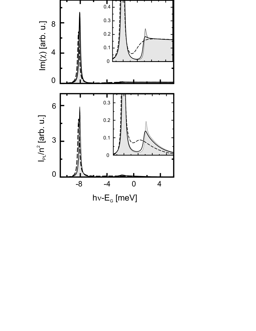
Figure 1: Absorption (top) and PL spectra (bottom) for a carrier temperature of $T=40$ K for three different carrier densities of $n=5\times 10^{8}$ cm^-2 (shaded area), $n=1\times 10^{9}$ cm^-2 (solid line), and $n=6\times 10^{9}$ cm^-2 (dashed line). The insets show the magnification of the region around the $2s$ resonance.

We first illustrate the influence of the microscopic scattering on the higher bound states by evaluating the fully microscopic absorption and PL spectra for various carrier densities. More specifically, we assume Fermi-Dirac distributions at 40 K for electrons and holes and take three very low values for the densities which are usually all considered to be in the “linear regime”. In addition to the microscopic Coulomb scattering, we have included a small background $\gamma=0.125$  meV which results from the effects of acoustic phonon scattering and the purely radiative decay. Figure 1 presents absorption and PL spectra side by side showing that the $1s$-exciton resonance lies 8 meV below the band gap. For the densities used here, it is hardly changed and its width is basically determined by the background decay constant. But while the $1s$-exciton resonance is almost unchanged even for the largest density used here, the magnifications in the insets clearly demonstrate a very strong broadening of the 2s-exciton resonance. The absorption spectra show that the $2s$ resonance merges with the continuum already at around $10^{9}$ cm^-2, a density which is usually considered very low in typical GaAs-type QW systems. The same trend is visible in the PL spectra where it is almost impossible to detect a clear $2s$ resonance, instead it merely marks the onset of the exponential decay into the continuum. This fact explains why the $2s$ resonance is often not cleary observable in experiments.

The relation between excitonic resonances and nonlinearities can be investigated most easily if we define the separate contributions of Eqs. (31) and (35) via

$$\alpha(\omega) = \sum_{\nu}\alpha_{\nu}(\omega)$$ (41)

$$I^{{\mathrm{PL}}}(\omega) = \sum_{\nu}I^{{\mathrm{PL}}}_{\nu}(\omega)(\omega)$$ (42)

with

$$\alpha_{\nu}(\omega) \propto |d_{{\mathrm{cv}}}|^{2}\sum_{\mu}\frac{\varphi^{R}_{\nu}(r=0,\omega)\bigl{(}\varphi^{R}_{\mu}(r=0,\omega)\bigr{)}^{*}}{E_{\nu}(\omega)-\hbar\omega-i\Gamma_{\nu}(\omega)}A_{\nu,\mu}(\omega),$$ (43)

$$I^{{\mathrm{PL}}}_{\nu}(\omega) \propto |d_{{\mathrm{cv}}}|^{2}\sum_{\mu}\frac{\varphi^{R}_{\nu}(r=0,\omega)\bigl{(}\varphi^{R}_{\mu}(r=0,\omega)\bigr{)}^{*}}{E_{\nu}(\omega)-\hbar\omega-i\Gamma_{\nu}(\omega)}S_{\nu,\mu}(\omega).$$ (44)

Here, the individual contributions of the different exciton states $\nu$ appear separately. However, since the eigenenergies and broadenings are frequency dependent, this simple form is in fact somewhat misleading. Due to the frequency dependence of the complex excitonic eigenvalues the generalized Lorentzian function can in reality deviate quite strongly from a simple Lorentzian — even more so since in general the oscillator strength in the numerator can be complex and thus mix real and imaginary parts of the energy denominator.

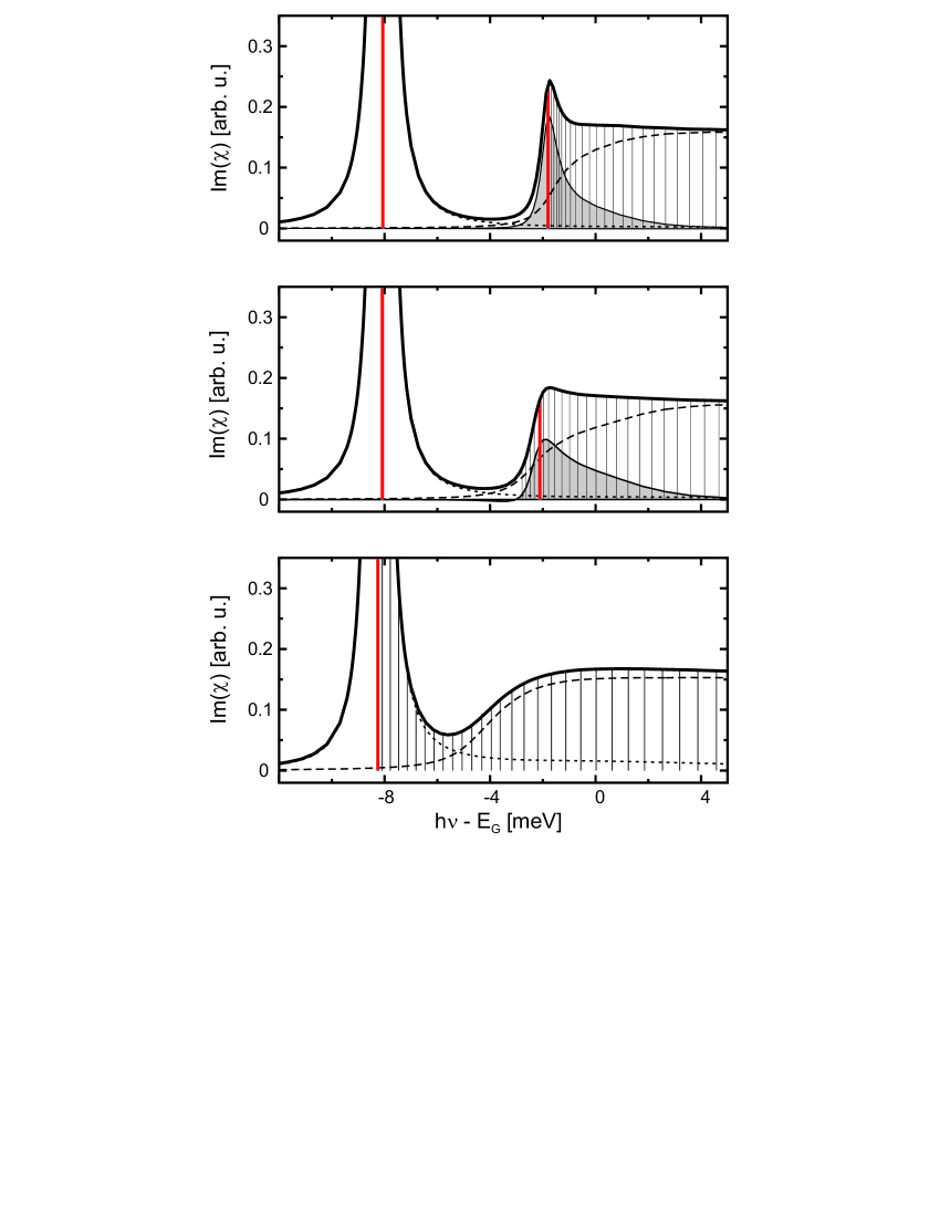
Figure 2: Absorption spectra for a carrier temperature of $T=40$ K for three different densities of $n=5\times 10^{8}$ cm^-2 (top), $n=1\times 10^{9}$ cm^-2 (middle), and $n=6\times 10^{9}$ cm^-2 (bottom). In addition to the full spectrum (solid line), the separate contribution for the $1s$ resonance (dotted line), the $2s$ resonance (shaded area), and the rest (dashed line) is given. The vertical lines display the real parts of the excitonic eigenenergies of the generalized Wannier Eq. (28).

In Fig. 2, we show the same three absorption spectra as in Fig. 1 as thick solid lines. But now, we also plot $\alpha_{1s}$, $\alpha_{2s}$ and the rest separately. Since the excitonic states have a complicated $\omega$ dependence due to the scattering matrices, we identified the $1s$ and $2s$ resonances by choosing at each $\omega$ those two excitonic states which have the highest oscillator strength. Especially for higher densities, we find an entire continuum of excitonic states; some of them have a relatively small oscillator strength. But a clear distinction of the different states, as in the zero-density analytical Wannier formula, is no longer possible.

Even for the lowest density, the $2s$ resonance is strongly non-Lorentzian and extends well into the continuum. Reversely, even the higher lying continuum states contribute significantly (almost a quarter) to the observed $2s$ peak. For the intermediate density, this effect becomes even more pronounced and for the highest density, it is no longer possible to determine a clear resonance. This becomes understandable if we look at the vertical lines in the figure which indicate the positions of the real parts of the eigenvalues. For low densities these real parts agree with the expected energies of the $1s$, $2s$ etc. states. However, we see that for elevated densities the microscopic scattering leads to resonances even between the $1s$ and $2s$ energies. For the highest density, these resonances can extend down to the $1s$ peak itself.

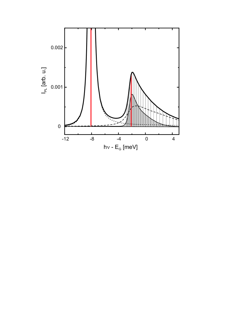
Figure 3: PL spectrum and the different contributions for the same parameters as the middle frame of Fig. 2.

Exactly the same analysis as before is performed for our PL spectra. For the intermediate density, the result is displayed in Fig. 3. All features discussed in Fig. 2 are clearly visible also here. The excitonic positions are the same as in the absorption analysis, since the exciton basis for semiconductor Bloch and luminescence equations are identical. As we have already mentioned in the discussion of Fig. 1 a clear $2s$ resonance cannot be distinguished. It is composed of a whole cluster of resonances and has to be analyzed with a full microscopic theory. A zero-density Wannier basis is clearly insufficient to understand these intricate effects.

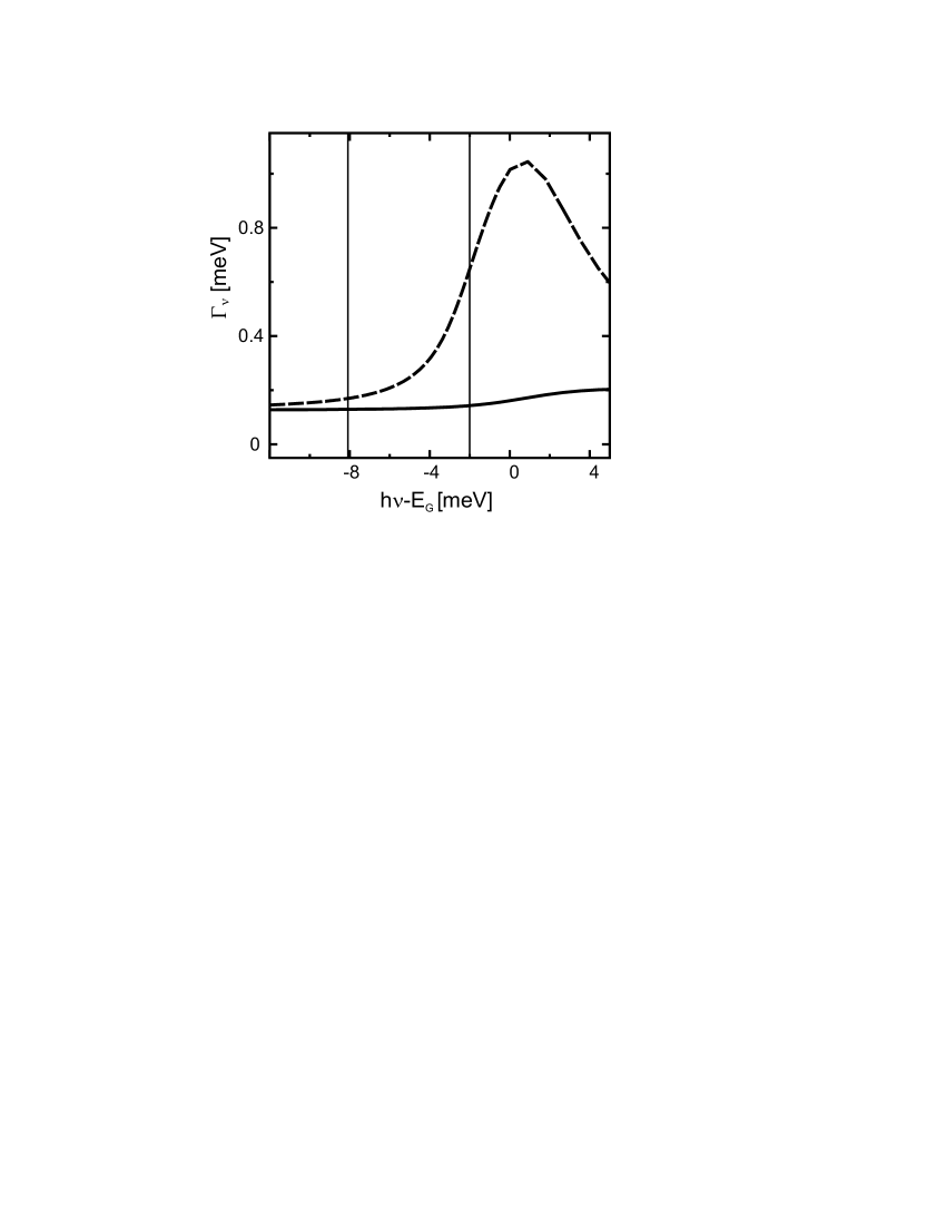
Figure 4: Imaginary part of excitonic eigenenergy of the generalized Wannier Eq. (28) for the two bound states with the hightest (solid line) and the second-highest (dashed line) oscillator strength for a carrier temperature of $T=40$ K and a carrier density of $n=1\times 10^{9}$ cm^-2. The vertical lines indicate the respective real parts.

Figure 4 presents an important part of the information necessary to understand the strong non-Lorentzian lineshape features. Here, we show the frequency dependence of the broadening of the two bound states with the highest oscillator strength. For simplicity, we continue to call the second resonance a $2s$ resonance in analogy to the usual Wannier nomenclature. Our observation from the spectra are confirmed here; while the $1s$ resonance is almost independent of frequency and dominated by the background decay constant $\gamma_{{\mathrm{bg}}}=0.125$ meV, the broadening of the second resonance is strongly frequency dependent. At the frequency value where the maxima of the corresponding resonances are observed (indicated by the vertical lines) the broadening of the second is already about five times as big as that of the first resonance. The fact that this broadening decays more quickly towards lower frequencies than towards higher frequencies explains the non-Lorentzian feature and the larger extension of the $2s$ resonance towards the continuum states. At the same time, the small $1s$ broadening is consistent with the observed narrow Lorentzian line from Figs. 1–3.

This explanation covers only part of the non-Lorentzian lineshape. By looking at Eqs. (31) and (35) we note that fundamentally the influence of scattering can be even more complicated. Since the presence of scattering generally leads to complex wave functions and correlations $A_{\nu,\mu}$ and $S_{\nu,\mu}$, even the oscillator strength can be complex and real and imaginary parts, i.e. broadened $\delta$-function and principal value contributions in the complex Lorentzian functions can be mixed.

Before turning our attention to more details of the PL spectra, we summarize the important finding of this section. We have noted that both in absorption and in PL the so-called “$2s$ resonance” actually consists of a whole cluster of energetically close resonances. Except for ultra-low densities the usual nomenclature fails and the $2s$ resonance is not necessarily the second lowest bound state. Microscopic Coulomb scattering leads to the presence of a continuum of states, sometimes even relatively close to the $1s$-exciton resonance.

III.2 Plasma luminescence spectra

Since we have seen in the previous section that the analysis of the $2s$ resonance is a rather delicate issue, we start our detailed investigation of PL spectra by comparing different approximations and their influence around the $1s$ resonance. This resonance is modified much less by Coulomb scattering than the $2s$ resonance such that we can anticipate it to be more robust under different approximations applied.

In the present section, all PL spectra are computed from Eq. (35) with the Hartree-Fock source, Eq. (37), and the correlated plasma contribution obtained from Eq. (26). We do not add additional diagonal exciton populations until the next section where the ratio between excitonic and plasma luminescence is investigated. For comparison, we also present solutions of the simplified Elliott formula, Eq. (39), where the decay constant is chosen such as to match the width of the $1s$ resonance of the full computation. Within the Elliott formula approach, there are three different possibilities to deal with the four-point $c_{X}$ correlations. The best and most consistent way is the full solution of Eq. (26) with the scattering matrices replaced by a constant $\gamma$. The other two possibilities truncate already part of the four-point terms and can thus lead to inconsistencies at higher bound or continuum states. We include them here for comparison only and in order to relate previous results to the full theory. In the simplest case, we can neglect the $c_{X}$ correlations completely. Then we obtain spectra in the same approximation as in our first publicationsKira et al. (1997b), referred to in the present paper as “Hartree-Fock” approximation. We can improve this approximation by solving the four-point correlations in a scattering approach as has been discussed in Sec. 4.4 of Ref. Kira et al., 1999. In that case, the four-point correlations are obtained as

$$c^{0,{\bf k}^{\prime}_{\|},{\bf k}_{\|}}_{\rm X}\Bigr{|}_{{\mathrm{scat}}}=\frac{-S^{0,{\bf k}^{\prime}_{\|},{\bf k}_{\|}}}{\epsilon^{{\bf q}_{\|},{\bf k}^{\prime}_{\|},{\bf k}_{\|}}-i\gamma}$$ (45)

with the definitions from Eqs. (5) and (8). As can be seen from the energy denominator, Coulomb resonances are not included in the description of the electron-hole correlations in that approximation. Hence, we have four different ways to calculate the $1s$ PL: the fully consistent plasma result from Eq. (26) with microscopic scattering matrices, the same with a constant $\gamma$ approximation (Elliott), and then two approximations where either Eq. (26) is truncated and solved without the Coulomb sums (scattering approximation) or where the four-point correlations are neglected completely (Hartree-Fock).

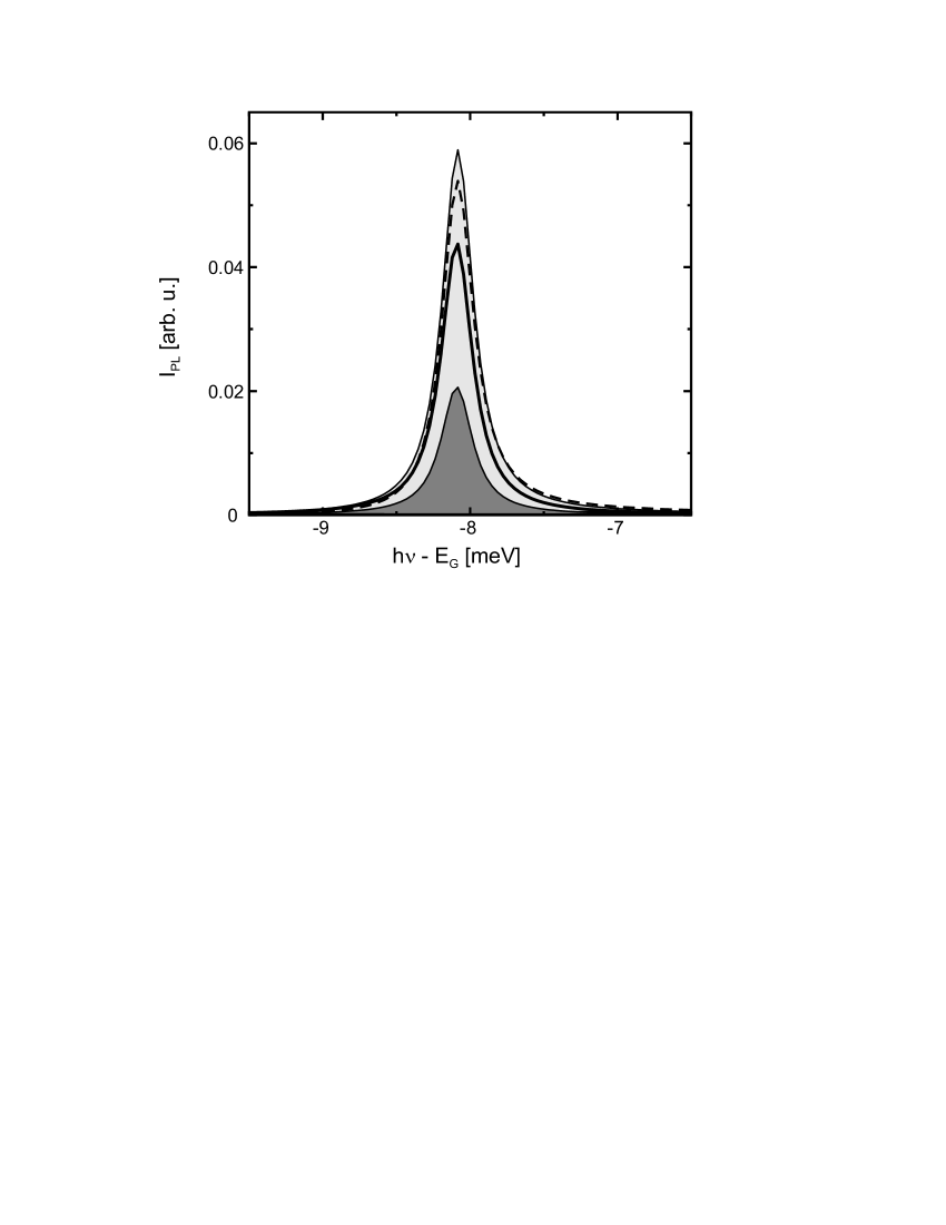
Figure 5: PL spectrum in the spectral vicinity of the $1s$ resonance. The full result from Eq. (35) (shaded area) is compared to three different approximations of the Elliott formula with constant dephasing, Eq. (39). Here, the correlated PL source term is treated fully (solid line), in scattering approximation (dashed line), or set to zero (Hartree-Fock approximation, dark-shaded area). The constant-gamma results have been shifted by 40 $\mu$eV in order to collocate the peaks at the same frequency.

Figure 5 presents the PL spectra around the $1s$ resonance for these four different ways of computing the excitonic correlations. All approximations exhibit a clear peak at the $1s$ resonance. A small shift of 40 $\mu$eV for the three constant-gamma calculations compensates small differences in the energy renormalizations with and without microscopic scattering. While the Hartree-Fock approximation gives only about one third of the full plasma PL, the other two approximations are within 30% of the full plasma value. Since we adjusted the decay constant, we can directly compare the peak heights in order to compare the quality of the different approximations. This is done in detail in Fig.6 for the two carrier temperatures of $T=20$ K and $T=60$ K. For both temperatures, the Eliott formula approaches the full plasma PL for very low densities, deviates most strongly at some intermediate densities, before getting better again in the limit of higher densities. The maximum deviation is temperature dependent and is less than 40% for 20 K and even smaller around 25% for 60 K. The Hartree-Fock approximation shows a similar functional form, but is in general too small by a factor of around three to four, with the precise value also depending on carrier density and temperature. The scattering approximation decays monotonously from low to high densities. For very low densities, it can even overestimate the correct value of the plasma luminescence as can be anticipated by extrapolating the curve to zero density. For high densities, it is too small by less than a factor of two.

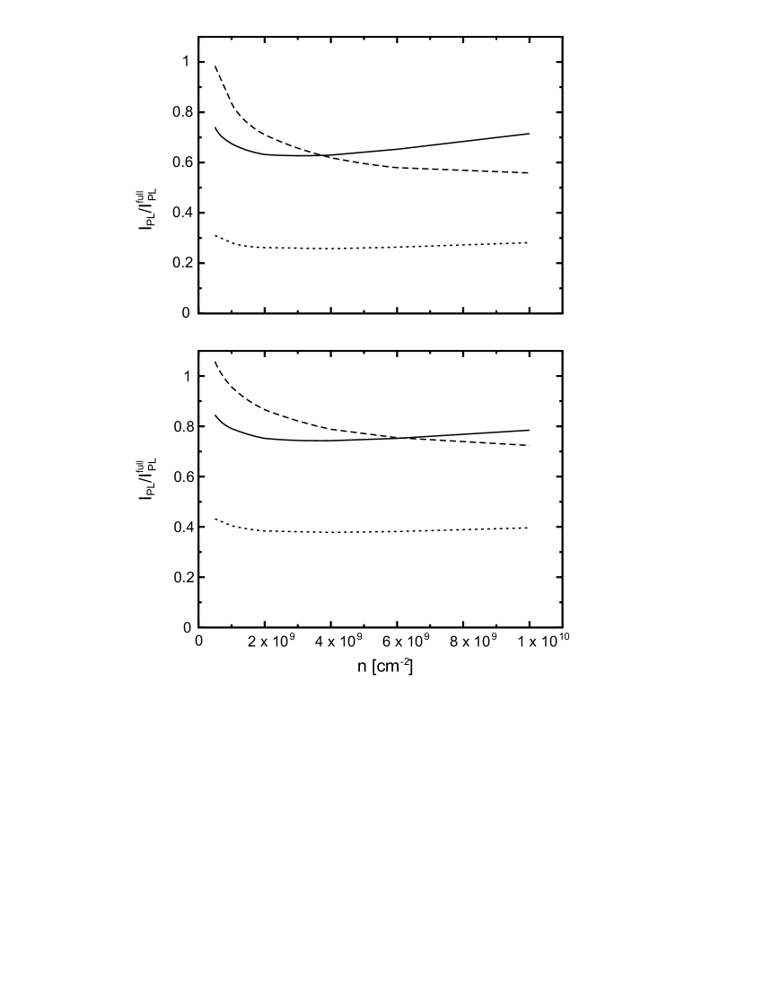
Figure 6: Relative peak height of Elliott formula (solid line), second-Born source (dashed line), and Hartree-Fock source term (dotted line) relative to the peak height of the full plasma result with microscopic scattering. Results for carrier temperature of $T=20$ K (top) and $T=60$ K (bottom) are shown.

III.3 Excitonic plasma luminescence

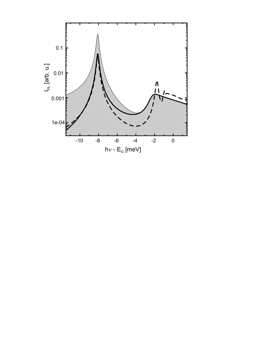
Figure 7: PL spectra for the same parameters as in Fig. 5 in semilogarithmic plot. The full plasma PL (solid line) and the Elliott-formula result are compared to the thermodynamic limit (shaded area).

The results in Sec. III.2 show that the intensity of the $1s$-plasma PL can be predicted rather accurately using different levels of approximations. We next quantify the characteristics of the $1s$ PL with respect to other resonances in the spectrum. Especially, we may use the thermodynamic relation (21) between $\alpha(\omega)$ and ${\rm PL}(\omega)$ to define how nonthermal the excitonic plasma PL is. The computed full (solid line), Elliot (dashed line), and thermodynamic (shaded area) PL are presented in Fig. 7. Here, the carrier density has been taken as $10^{9}{\rm cm}^{-2}$ and the lattice temperature is 40 K. The shown thermodynamic PL is simply obtained by computing the microscopic absorption from Eq. (31). Then, $\alpha(\omega)$ is multiplied by a thermal factor according to Eq. (21). The temperature is chosen such that the high-energy PL tails of the full and the thermodynamic computations agree.

We observe now that event though the full and the Elliot PL agree at the $1s$ resonance, the Elliot PL overestimates the high-frequency part of the spectrum since microscopic Coulomb scattering is not included. This is a clear indication that one needs to include the microscopic scattering to understand the quantitative features in the full spectral range of the excitonic PL. A comparison of the full and the thermodynamic PL indicates that the excitonic plasma PL is strongly nonthermal since it produces a much weaker $1s$ resonance than thermodynamic arguments predict. We will see, later on, that one actually needs true $1s$-exciton populations to enhance the $1s$ PL toward its thermodynamic value. The inherent nonequilibrium feature of the excitonic plasma luminescence has a simple explanation. It is intuitively clear that $1s$ emission from plasma or correlated electron-hole plasma is more complicated than from exciton populations. This complication arises from the fact that an electron-hole plasma can emit a photon at excitonic frequencies, which are much below its average energy per particle, only by heating the remaining plasma. Due to this additional difficulty, the excitonic PL resulting from a pure plasma is generally weaker than that for the pure thermodynamic limit containing also exciton populations.

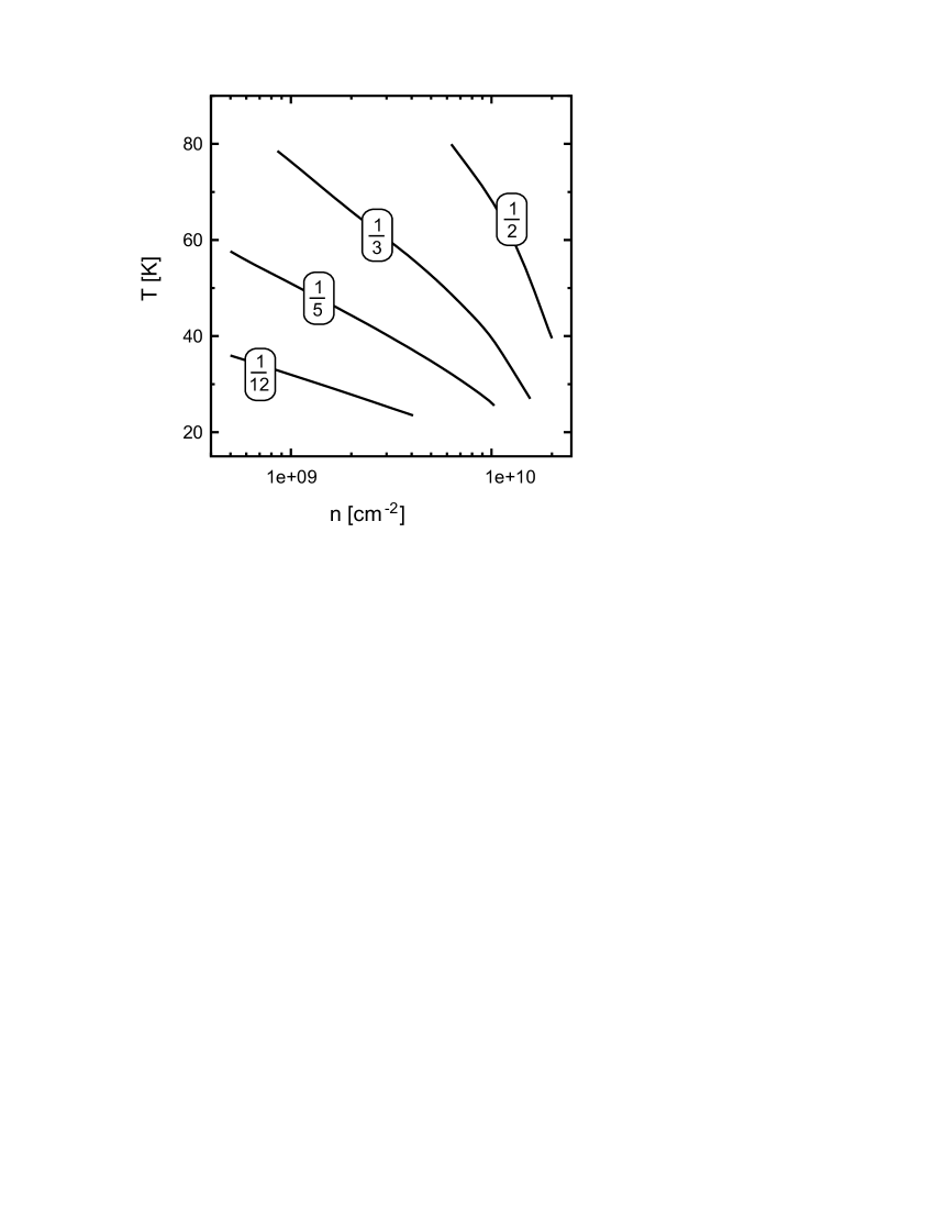
Figure 8: “Phase-space” plot for $\beta$-factor as function of carrier density and temperature. The temperature has been determined from the continuum tail of the emission.

To quantify the level of nonthermal character in more detail, we define a $\beta$ suppression factor,

$$\beta\equiv\frac{{\rm PL}_{1s}|_{\rm full}}{{\rm PL}_{1s}|_{\rm TD}},,$$ (46)

first introduced by Schnabel et al.Schnabel et al. (1992). Essentially, the $\beta$ factor tells us how strongly the actual $1s$ PL, ${\rm PL}_{1s}|_{\rm full}$, is suppressed with respect to its thermodynamic value ${\rm PL}_{1s}|_{\rm TD}$. Figure 8 presents a contour plot of $\beta$ as function of carrier density and temperature when only the fully mictroscopically included plasma luminescence is included. As a general tendency, the plasma PL becomes strongly nonthermal for low densities and temperatures. This is the regime which is favourable to sustain truly bound excitons. As temperature and/or density are increased, the excitonic plasma PL approaches the thermodynamic limit.

As a general tendency, the $\beta$ analysis has a rather weak sensitivity to the scattering model used or to low levels of disorder.Bozsoki et al. (2006) Thus, the $\beta$ analysis is very much suitable to analyze the plasma nature of experimentally detected PL. In other words, the presented $\beta$-phase diagram can be applied to diagnose the degree to which the measured PL in low-disorder GaAs-type samples is caused by plasma emission. On the basis of a quantitative analysis of simultaneously measured PL and absorption, Refs. Chatterjee et al. (2004); Hoyer et al. (2005b) have shown that the experimental results for temperates above 30 K and densities above $5\times 10^{9}{\rm cm}^{-2}$ can be attributed to pure plasma emission.

III.4 Exciton-population effects

Under suitable conditions a system of incoherent electron-hole quasi-particle excitations consists a mixture of correlated electron-hole plasma and exciton populations. Clearly, exciton populations may appear in all exciton states including the ionization continuum. In particular, the full thermodynamic equilibrium between plasma and excitons leads to a many-body problem Portnoi and Galbraith (1999); Siggelkow et al. (2004) that produces highly nontrivial many-body states. However, several recent experiments Schnabel et al. (1992); Chatterjee et al. (2004); Hoyer et al. (2005b) demonstrate that excitonic PL is almost always far from the purely thermodynamic limit. Thus, it seems realistic to assume that the correlated electron-hole plasma coexists together with a fraction of excitons that is determined by the exciton formation kinetics and typically much below its thermodynamic value. Since the $1s$-exciton populations dominate at low temperatures, we include only them in our analysis of the exciton population contribution to the PL.

As discussed in Sec. III.3, the PL at the $1s$ resonance can be strongly enhanced by the presence of true exciton populations. This can be seen directly from the luminescence Elliot formula (39). More precisely, a $1s$-exciton population basically adds luminescence at the $1s$ frequency whose magnitude increases as a linear function of the exciton occupation $\Delta N_{1s}$. In order to investigate this effect, we add $1s$ exciton populations to the fully microscopically computed correlated plasma luminescence. We assume that the added $1s$ excitons have a thermal momentum distribution such that $\Delta N_{1s}(0)$, i.e. the ’bright part’ of the exciton distribution that contributes to the luminescence in normal direction, is known. In practice, the population $\Delta N_{1s}(0)$ is added to the source (25) such that the fully microscopic luminescence is solved from Eqs. (35) for the coexisting exciton and plasma populations.

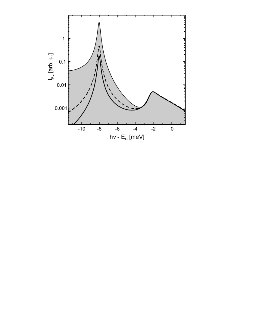
Figure 9: PL spectra for a carrier density of $n=1\times 10^{9}$ cm^-2 and a nominal carrier temperature of $T=20$ K. The full plasma result (solid line) is compared to the thermodynamic curve (shaded area). Adding 1% excitons at a temperature of $T_{X}=10$ K (dashed line) drastically increases the $1s$ PL.

To illustrate the basic effect of exciton populations, we assume a low carrier density of $10^{9}{\rm cm}^{-2}$ and 20 K carrier temperature. Since the excitons can often reach a lower temperature than the carrier distributions, we choose a 10 K temperature for the excitons. Figure 9 shows PL without excitons (solid line), 1% excitons (dashed line), and the thermodynamic limit (shaded area). We notice that in all cases, the PL spectra are qualitatively similar, especially, the PL above the second resonance is virtually the same. Hence, the main feature of $1s$ populations is that they increase the $1s$ PL toward the thermodynamic limit. This confirms our previous assumption that exciton populations must be included to produce a thermodynamic PL.

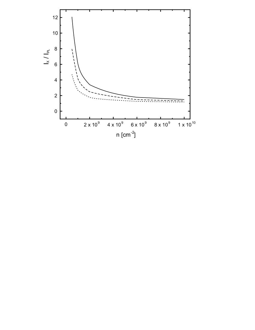
Figure 10: Ratio between $1s$ PL with and without an added amount of 1% excitons. For an excitonic temperature of $T_{X}=10$ K, the carrier temperature is $T=40$ K (solid line), $T=30$ K (dashed line), and $T=20$ K (dotted line).

We investigate next how much the $1s$ PL is changed by a 1% fraction of $1s$ excitons as function of total carrier density. As in Fig. 9, we assume a 10 K exciton temperature. For each density, we define the ratio of the $1s$ peak heights,

$$R_{X}\equiv\frac{{\rm PL}_{1s}|_{\rm X}}{{\rm PL}_{1s}|_{\rm full}},,$$ (47)

between the case with excitons, ${\rm PL}_{1s}|_{\rm X}$, and without, ${\rm PL}_{1s}|_{\rm full}$, producing the microscopic plasma PL. The results are shown in Fig. 10 as function of carrier density for 20 K (solid line), 30K (dashed line), and 40 K (dotted line) carrier temperature. The exciton populations have strongest effect at low densities while $R_{X}$ approaches unity for the elevated densities. This is in agreement with our earlier observation that high temperature plasma PL tends to approach the thermodynamic limit, i.e., excitons are then less important. However, we observe a strong increase of $R_{X}$ for low densities and temperatures. According to Eq. (39), the low-density plasma PL scales with the product of the carrier occupations, $f^{e}f^{h}$, while the exciton population PL is directly proportional to the occupation $\Delta N_{1s}$. When the carrier temperature is increased or the carrier density is decreased, the absolute magnitude of the plasma PL decreases nonlinearly. If the exciton occupation has a fixed temperature, as we have assumed in Fig. 10, the relative strength of the population PL increases with respect to the plasma PL as the density is lowered or the carrier temperature is increased. Thus, the observed increase of $R_{X}$ follows directly from the nonlinear dependence of the plasma PL for low densities. In particular, the exciton populations can contribute strongly under low temperature and low density conditions as verified in recent experiments.Chatterjee et al. (2004); Hoyer et al. (2005b)

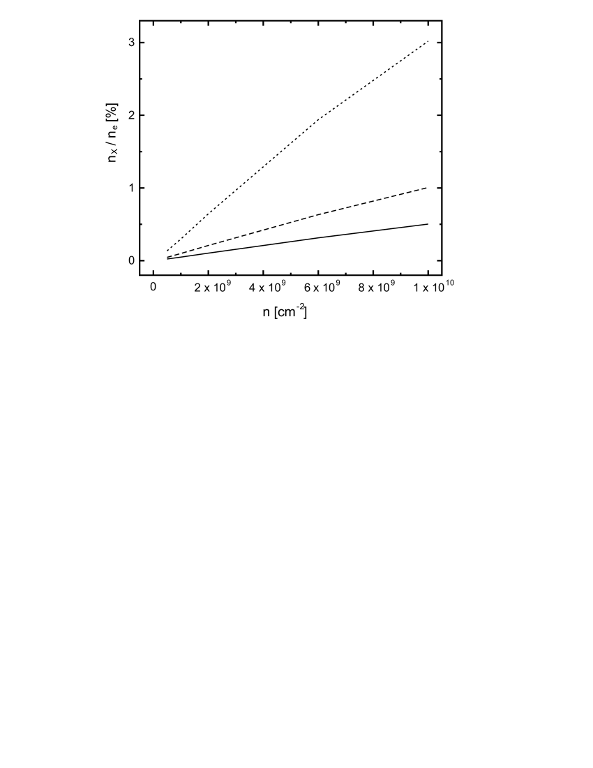
Figure 11: Necessary exciton fraction to be added in order to obtain a ratio of 3/2 between the $1s$-resonance peaks with and without additional excitons. For an excitonic temperature of $T_{X}=10$ K, the carrier temperature is $T=60$ K (solid line), $T=40$ K (dashed line), and $T=20$ K (dotted line).

The effect of $1s$ populations can also be investigated by evaluating how large an exciton fraction,

$$x^{50\%}_{1s}\equiv\frac{\Delta n_{1s}|_{50\%}}{n_{eh}},$$ (48)

is needed to increase the excitonic $1s$ luminescence by 50%. As in Fig. 10, we assume that the $1s$-exciton distributions follow a thermal Bose-Einstein distribution at a temperature of 10 K. We assume carrier temperatures of 20 K (solid line), 40 K (dashed line), and 60 K (dotted line) and define $x^{50\%}_{1s}$ as function of density. The result is displayed in Fig. 11. We observe again that low carrier densities are sensitive to the presence of exciton populations while their effect becomes less important for elevated temperatures and densities. The difference of low vs. high temperature can be understood on the basis of the same nonlinearity arguments as in Fig. 10.

IV Discussion and Conclusion

Excitonic PL resulting from an electron-hole plasma has been observed in a variety of experiments performed with GaAs-type QW systems. For example, the ultrafast build up of the $1s$-luminescence resonance on a subpicosecond time scale REF is a clear indication of emission from a relaxing electron-hole plasma. The formation times of incoherent exciton poplulations are much longer. This has been carefully analyzed recently in experiments where absorption and PL spectra have been measured simultaneously.Chatterjee et al. (2004); Hoyer et al. (2005b) The microscopic analysis of these experiments not only verify that excitons are formed on a time scale of several hundred picoseconds but they also showed that appreciable exciton populations are obtained only for temperatures below 30 K and densities below $10^{10}$ cm^-2. Otherwise, the excitonic PL could be explained by our plasma PL alone.

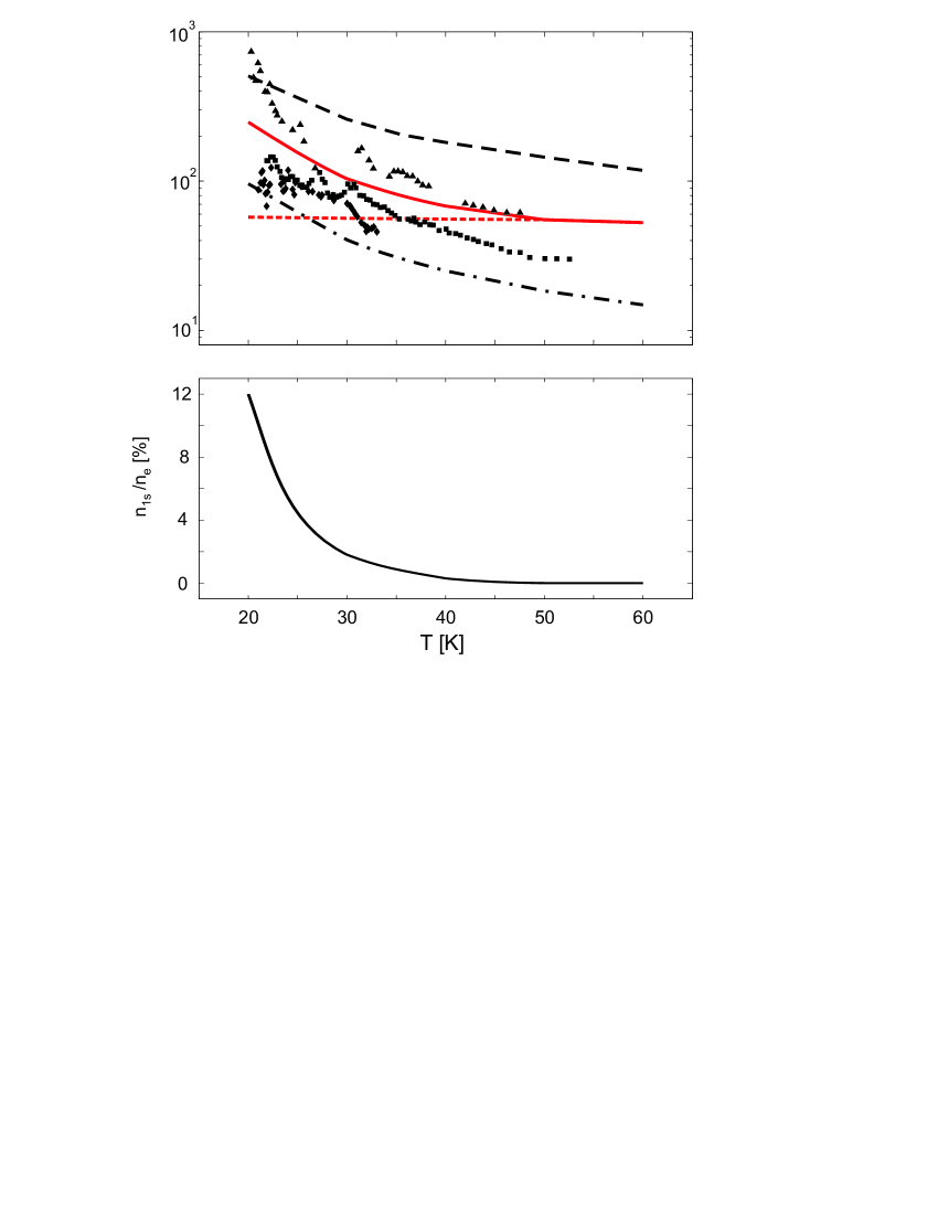
Figure 12: Top: A comparison between the data points from Fig. 5 of Phys. Rev. B 71, 195313 (2005) and the thermodynamic result as obtained from analysing either peak heights (dashed) or areas (dot-dashed line) of $1s$ and higher resonances, respectively. Our result without (dotted) and with (solid) added excitons obtained from the peak-height analysis has been added. Bottom: Necessary exciton fraction for an excitonic temperature of $T_{X}=10$ K used for the top part of the figure.

In order to check these interpretations, we analyze the experimental data published recently in Ref. Szczytko et al. (2005). In Fig. 12, we have carefully read in all experimental data points from Fig. 5 in Ref. Szczytko et al. (2005) We compare these date to our full theory and several levels of approximation. We first compute the $1s$-to-$2s$ ratio by integrating the thermodynamic result, Eq. (21), obtained from our absorption spectrum for a density of $10^{9}$ cm^-2. If we determine the ratio by integrating a spectral range of $8\,meV$ around each resonance as has bene done in Ref. Szczytko et al., 2005, we obtain the dot-dashed line; if we plot the peak ratio instead, we get the dashed line. The area ratio lies well below almost all of the experimental data points. One can think of a large variety of possible explanations, which include radiative effects (the sample is measured in reflection geometry in front of a distributed-Bragg-mirror) or possible disorder effects which could potentially enhance the $1s$ emission relative to the rest. In order to proceed with our analysis, we therefore use the peak ratio as a reference, which lies clearly above most of the experimental data points. The results of our luminescence theory for various temperatures is plotted in Fig. 12 before and after adding additional excitons to our plasma PL. The necessary fraction of excitons needed to obtain our fit is given in the bottom panel. Already the plasma theory nicely agrees with the experimental results for elevated temperatures above 40 K. And for lower temperatures we find that exciton populations do indeed contribute significantly. Even though we do not have access to the full experimental information, this comparison shows that the experimental results can be well explained with our theory, in contrast to the claims in Ref. Szczytko et al., 2005. For a detailed one-to-one analysis, the carrier density for each data point should be obtained in the experiment as well.

As an alternative experimental route, also THz experimentsKaindl et al. (2003) performed under similar conditions show unambiguously that $1s$-exciton populations are formed on a nanosecond time scale. Recently, also a combination of PL and THz absorption measurements has been reported.Galbraith et al. (2005) There it has been shown that a $1s$-exciton resonance can indeed be seen in the PL even when THz absorption does not exhibit a $1s-2p$ resonance indicating unambiguously that $1s$-exciton populations are not present under these conditions.

Both the strong non-thermal nature of PL spectra and the excitonic PL without a corresponding THz absorption signal can easily be explained if one includes the plasma PL in the analysis. While varying in importance, this contribution is fundamentally always present since it only requires that carrier distributions are excited. The strength of the present theory is to simultaneously treat effects from both the electron-hole plasma and the excitons by fully including the Fermionic substructure of the excitons. Only such a combined analysis without exclusive restriction to one of the possible emission sources can answer the question which source is important under given experimental conditona.

To summarize, in the present paper we have discussed and evaluated our microscopic theory for calculating PL spectra of semiconductor QW systems and for analyzing exciton and plasma contributions to luminescence, respectively. We have particularly focused on the effects of microscopic Coulomb scattering and analyzed their influence on the different exciton resonances. While the PL Elliott formula, Eq. (39), elucidates the underlying physics, a realistic theory-experiment comparison should always include microscopic scattering, in particular if the detailed structure around the band-edge is of special interest. A desirable extension of our theory would be to simultaneously include the exciton formation dynamics and the PL in a systematic way. Even though the theoretical framework exists, the numerical implementation of such a theory is very demanding and requires a lot of additional work and improved computer resources.

Appendix A Mathematical description of excitons

Based on the four-point definition in Sec. II.1, we find a natural way to identify incoherent excitons once we evaluate the electron-hole pair-correlation function

$$g_{\rm eh}({\bf r}_{\|})\equiv\langle{\Psi}^{\dagger}_{e}({\bf r}_{\|})\Psi^{\dagger}_{h}(0)\Psi_{h}(0){\Psi}_{e}({\bf r}_{\|})\rangle,$$ (49)

$${\Psi}_{e}({\bf r}_{\|})=\frac{1}{\sqrt{\sf S}}\sum_{{\bf k}_{\|}}a_{c,{\bf k}_{\|}}e^{i{\bf k}_{\|}\cdot{\bf r}_{\|}},\;\;\;\;{\Psi}^{\dagger}_{h}({\bf r}_{\|})=\frac{1}{\sqrt{\sf S}}\sum_{{\bf k}_{\|}}a_{v,{\bf k}_{\|}}e^{i{\bf k}_{\|}\cdot{\bf r}_{\|}},$$ (50)

where only the envelope part of the field operator $\hat{\Psi}_{\lambda}({\bf r}_{\|})$ is included since the Wannier excitons depend on a length scale much longer than the lattice periodic part of the Bloch functions. In general, $g_{\rm eh}({\bf r}_{\|})$ defines the conditional probability to find an electron at position ${\bf r}_{\|}$ when the hole is positioned at the origin. Thus, properties of $g_{\rm eh}({\bf r}_{\|})$ can identify what kind of correlations one can observe in the relative coordinate between the electrons and holes in the many-body system.

The pair-correlation function can always be divided into single-particle as well as to correlated two-particle contributions and the homogeneous incoherent quasiparticle excitation conditions produce

$$g_{\rm eh}({\bf r}_{\|})\equiv n_{e}n_{h}+\Delta g_{\rm eh}({\bf r}_{\|}),$$ (51)

$$\Delta g_{\rm eh}({\bf r}_{\|})\equiv\frac{1}{{\sf S}^{2}}\sum_{{\bf k}_{\|},{\bf k}^{\prime}_{\|},{\bf q}_{\|}}c_{X}^{{\bf q}_{\|},{\bf k}^{\prime}_{\|},{\bf k}_{\|}}e^{i({\bf k}^{\prime}_{\|}+{\bf q}_{\|}-{\bf k}_{\|})\cdot{\bf r}_{\|}}.$$ (52)

We observe now that the single-particle factorization leads to a background contribution, $n_{e}n_{h}$, which states that probability of finding electron and hole simultaneously is proportional to the product of their respective densities. This contribution does not have a genuine ${\bf r}_{\|}$-dependence. As a result, the true exciton effects are observed only in the correlated two-particle contributions $\Delta g_{\rm eh}({\bf r}_{\|})$ which contains exclusively the $c_{X}$ correlation. Thus, it is obvious now that only $c_{X}$ contributions can define and include the microscopic description of the true excitons in the many-body system.

The correlated $\Delta g_{\rm eh}({\bf r}_{\|})$ can also be expressed in the exciton basis

$$\Delta g_{\rm eh}({\bf r}_{\|})=\sum_{\lambda,\nu}\left({\frac{1}{\sf S}}\sum_{{\bf q}_{\|}}\Delta N_{\lambda,\nu}({\bf q}_{\|})\right)\left[\varphi^{R}_{\lambda}({\bf r}_{\|})\right]^{\star}\varphi^{R}_{\nu}({\bf r}_{\|}).$$ (53)

When $\Delta g_{\rm eh}({\bf r}_{\|})$ exhibits a clear single-state $r$-dependence proportional to $|\varphi^{R}_{\lambda_{0}}({\bf r}_{\|})|^{2}$, it is obvious that the $\sum_{\lambda,\nu}$ sum is dominated by the element $\lambda=\nu=\lambda_{0}$. Since this case corresponds to having only $\lambda_{0}$ excitons, we may conclude that

$$\Delta n_{\lambda_{0}}\equiv{\frac{1}{\sf S}}\sum_{{\bf q}_{\|}}\Delta N_{\lambda_{0},\lambda_{0}}({\bf q}_{\|})$$ (54)

defines the density of excitons in state $\lambda_{0}$ in the system.

Appendix B Microscopic scattering

In order to get a realistic density dependence for the saturation of different excitonic resonances, it is important to include Coulomb scattering on a microscopic level. For completeness, we start by investigating the scattering for computation of absorption spectra, i.e. for the microscopic polarizations $\langle P_{k}\rangle=\langle v^{\dagger}_{k}c_{k}\rangle$.

In the language of the cluster expansion, Coulomb scattering is provided by coupling of $n$-point expectation values to $(n+2)$-point expectation values. In the case of the microscopic polarization, we find

$$i\hbar\frac{\partial}{\partial t}\langle P_{k}\rangle\Bigr{|}_{{\mathrm{scatt}}} = \phantom{+}\sum_{k^{\prime},q}V_{q}\left(\Delta\langle v^{\dagger}_{k}c^{\dagger}_{k^{\prime}}c_{k^{\prime}+q}c_{k-q}\rangle-\Delta\langle v^{\dagger}_{k+q}c^{\dagger}_{k^{\prime}}c_{k^{\prime}+q}c_{k}\rangle\right)$$ (55)

$$+\sum_{k^{\prime},q}V_{q}\left(\Delta\langle v^{\dagger}_{k}v^{\dagger}_{k^{\prime}}v_{k^{\prime}+q}c_{k-q}\rangle-\Delta\langle v^{\dagger}_{k+q}v^{\dagger}_{k^{\prime}}v_{k^{\prime}+q}c_{k}\rangle\right).$$

This equation is still exact, and the level of approximation is determined by the precision with which we calculate the four-point correlations. Their dynamics is determined by an equation of the general form

$$i\hbar\frac{\partial}{\partial t}\Delta\langle 4\rangle=S[\langle 2\rangle]+T[\langle 2\rangle,\Delta\langle 4\rangle]+V[\Delta\langle 6\rangle],$$ (56)

where the four-point correlations are driven by a source term $S[\langle 2\rangle]$ containing only sums and products of two point terms (such as microscopic carrier occupations and polarizations), they are coupled to other four-point correlations in a complicated manner symbolized by $T[\langle 2\rangle,\Delta\langle 4\rangle]$ and they are themselves coupled to yet higher order terms due to the hierarchy problem. The scattering approximation to this equation is obtained if all coupling between four-point terms and to six-point terms is neglected and only the kinetic energy contribution and the two-point source term is kept on the right-hand side. Formally, the scattering solutions can thus be obtained from

$$i\hbar\frac{\partial}{\partial t}\Delta\langle 4\rangle\Bigr{|}_{{\mathrm{scatt}}}=(\tilde{\varepsilon}-i\delta)\Delta\langle 4\rangle+S[\langle 2\rangle],$$ (57)

where we have introduced a phenomenological dephasing constant $\delta$ in addition to the sum of renormalized free-particle energies $\tilde{\varepsilon}$.

More specifically, we obtain

$$i\hbar\frac{\partial}{\partial t}\Delta\langle v^{\dagger}_{k}c^{\dagger}_{k^{\prime}}c_{k^{\prime}+q}c_{k-q}\rangle=\left(\tilde{\varepsilon}^{e}_{k-q}+\tilde{\varepsilon}^{h}_{k}+\tilde{\varepsilon}^{e}_{k^{\prime}+q}-\tilde{\varepsilon}^{e}_{k^{\prime}}-i\delta\right)\Delta\langle v^{\dagger}_{k}c^{\dagger}_{k^{\prime}}c_{k^{\prime}+q}c_{k-q}\rangle+S_{k,k^{\prime},q}$$ (58)

with the singlet source given by

$$S_{k,k^{\prime},q} = (V_{q}-V_{q+k^{\prime}-k})\left(f^{e}_{k^{\prime}}(1-f^{e}_{k^{\prime}+q})(1-f^{e}_{k-q})+(1-f^{e}_{k^{\prime}})f^{e}_{k^{\prime}+q}f^{e}_{k-q}\right)\langle P_{k}\rangle$$ (59)

$$-V_{q}\left(f^{e}_{k^{\prime}}(1-f^{e}_{k^{\prime}+q})(1-f^{h}_{k})+(1-f^{e}_{k^{\prime}})f^{e}_{k^{\prime}+q}f^{h}_{k}\right)\langle P_{k-q}\rangle$$

$$+V_{q+k^{\prime}-k}\left(f^{e}_{k^{\prime}}(1-f^{h}_{k})(1-f^{e}_{k-q})+(1-f^{e}_{k^{\prime}})f^{h}_{k}f^{e}_{k-q}\right)\langle P_{k^{\prime}+q}\rangle.$$

Here, we have neglected source terms in third order in $\langle P_{k}\rangle$ which is suitable for a low intensity probe pulse. In general, we want to calculate the susceptibility for a specific carrier density in a pump-probe type experiment relatively long (up to nanoseconds) after the pump pulse. After the fast initial scattering, the carrier distributions are known to be changing very slowly and can thus be assumed constant. In that case, we do not have to apply the Markov and random-phase approximation as has often been done in the past. Instead, we see that the quantity $\Gamma_{k}(\omega)$ which we introduced in the main part of the paper in Eq. (17), is nothing but the Fourier transform of the right-hand side of Eq. (55). This quantity can be split into two parts, $\Gamma^{c}_{k}$ and $\Gamma^{v}_{k}$, corresponding to the first and second line of Eq. (55), respectively.

Beginning with the computation of $\Gamma^{c}_{k}$, we need the Fourier transform of Eq. (58) which can be formally solved exactly via

$$\Delta\langle v^{\dagger}_{k}c^{\dagger}_{k^{\prime}}c_{k^{\prime}+q}c_{k-q}\rangle(\omega)=\frac{S_{k,k^{\prime},q}(\omega)}{\hbar\omega-\tilde{\varepsilon}^{e}_{k-q}-\tilde{\varepsilon}^{h}_{k}-\tilde{\varepsilon}^{e}_{k^{\prime}+q}+\tilde{\varepsilon}^{e}_{k^{\prime}}+i\delta}.$$ (60)

In a similar manner, we obtain

$$\Delta\langle v^{\dagger}_{k+q}c^{\dagger}_{k^{\prime}}c_{k^{\prime}+q}c_{k}\rangle(\omega)=\frac{S_{k+q,k^{\prime},q}(\omega)}{\hbar\omega-\tilde{\varepsilon}^{e}_{k}-\tilde{\varepsilon}^{h}_{k+q}-\tilde{\varepsilon}^{e}_{k^{\prime}+q}+\tilde{\varepsilon}^{e}_{k^{\prime}}+i\delta}.$$ (61)

With these ingredients, we can calculate $\Gamma^{c}_{k}$ by summing over Eqs. (60) and (61), using the definition of Eq. (59),

$$\Gamma^{c}_{k} = \phantom{+}\sum_{k^{\prime},q}\frac{V_{k-q}}{\hbar\omega-\tilde{\varepsilon}^{e}_{q}-\tilde{\varepsilon}^{h}_{k}-\tilde{\varepsilon}^{e}_{k^{\prime}}+\tilde{\varepsilon}^{e}_{k^{\prime}+q-k}+i\delta}\times$$ (62)

$$\Bigl{\{}(V_{k-q}-V_{k^{\prime}-k})\left(f^{e}_{k^{\prime}+q-k}(1-f^{e}_{k^{\prime}})(1-f^{e}_{q})+(1-f^{e}_{k^{\prime}+q-k})f^{e}_{k^{\prime}}f^{e}_{q}\right)\langle P_{k}\rangle$$

$$-V_{k-q}\left(f^{e}_{k^{\prime}+q-k}(1-f^{e}_{k^{\prime}})(1-f^{h}_{k})+(1-f^{e}_{k^{\prime}+q-k})f^{e}_{k^{\prime}}f^{h}_{k}\right)\langle P_{q}\rangle$$

$$+V_{k^{\prime}-k}\left(f^{e}_{k^{\prime}+q-k}(1-f^{h}_{k})(1-f^{e}_{q})+(1-f^{e}_{k^{\prime}+q-k})f^{h}_{k}f^{e}_{q}\right)\langle P_{k^{\prime}}\rangle\Bigr{\}}$$

$$-\sum_{k^{\prime},q}\frac{V_{k-q}}{\hbar\omega-\tilde{\varepsilon}^{e}_{k}-\tilde{\varepsilon}^{h}_{q}-\tilde{\varepsilon}^{e}_{k^{\prime}}+\tilde{\varepsilon}^{e}_{k^{\prime}+k-q}+i\delta}\times$$

$$\Bigl{\{}(V_{q-k}-V_{k^{\prime}-q})\left(f^{e}_{k^{\prime}+k-q}(1-f^{e}_{k^{\prime}})(1-f^{e}_{k})+(1-f^{e}_{k^{\prime}+k-q})f^{e}_{k^{\prime}}f^{e}_{k}\right)\langle P_{q}\rangle$$

$$-V_{k-q}\left(f^{e}_{k^{\prime}+k-q}(1-f^{e}_{k^{\prime}})(1-f^{h}_{q})+(1-f^{e}_{k^{\prime}+k-q})f^{e}_{k^{\prime}}f^{h}_{q}\right)\langle P_{k}\rangle$$

$$+V_{k^{\prime}-q}\left(f^{e}_{k^{\prime}+k-q}(1-f^{h}_{q})(1-f^{e}_{k})+(1-f^{e}_{k^{\prime}+k-q})f^{h}_{q}f^{e}_{k}\right)\langle P_{k^{\prime}}\rangle\Bigr{\}}$$

The other quantity $\Gamma^{v}_{k}$ can be obtained by symmmetry considerations. By exchaning each electron and hole index, we find

$$\Gamma^{v}_{k} = \phantom{+}\sum_{k^{\prime},q}\frac{V_{k-q}}{\hbar\omega-\tilde{\varepsilon}^{h}_{q}-\tilde{\varepsilon}^{e}_{k}-\tilde{\varepsilon}^{h}_{k^{\prime}}+\tilde{\varepsilon}^{h}_{k^{\prime}+q-k}+i\delta}\times$$ (63)

$$\Bigl{\{}(V_{k-q}-V_{k^{\prime}-k})\left(f^{h}_{k^{\prime}+q-k}(1-f^{h}_{k^{\prime}})(1-f^{h}_{q})+(1-f^{h}_{k^{\prime}+q-k})f^{h}_{k^{\prime}}f^{h}_{q}\right)\langle P_{k}\rangle$$

$$-V_{k-q}\left(f^{h}_{k^{\prime}+q-k}(1-f^{h}_{k^{\prime}})(1-f^{e}_{k})+(1-f^{h}_{k^{\prime}+q-k})f^{h}_{k^{\prime}}f^{e}_{k}\right)\langle P_{q}\rangle$$

$$+V_{k^{\prime}-k}\left(f^{h}_{k^{\prime}+q-k}(1-f^{e}_{k})(1-f^{h}_{q})+(1-f^{h}_{k^{\prime}+q-k})f^{e}_{k}f^{h}_{q}\right)\langle P_{k^{\prime}}\rangle\Bigr{\}}$$

$$-\sum_{k^{\prime},q}\frac{V_{k-q}}{\hbar\omega-\tilde{\varepsilon}^{h}_{k}-\tilde{\varepsilon}^{e}_{q}-\tilde{\varepsilon}^{h}_{k^{\prime}}+\tilde{\varepsilon}^{h}_{k^{\prime}+k-q}+i\delta}\times$$

$$\Bigl{\{}(V_{q-k}-V_{k^{\prime}-q})\left(f^{h}_{k^{\prime}+k-q}(1-f^{h}_{k^{\prime}})(1-f^{h}_{k})+(1-f^{h}_{k^{\prime}+k-q})f^{h}_{k^{\prime}}f^{h}_{k}\right)\langle P_{q}\rangle$$

$$-V_{k-q}\left(f^{h}_{k^{\prime}+k-q}(1-f^{h}_{k^{\prime}})(1-f^{e}_{q})+(1-f^{h}_{k^{\prime}+k-q})f^{h}_{k^{\prime}}f^{e}_{q}\right)\langle P_{k}\rangle$$

$$+V_{k^{\prime}-q}\left(f^{h}_{k^{\prime}+k-q}(1-f^{e}_{q})(1-f^{h}_{k})+(1-f^{h}_{k^{\prime}+k-q})f^{e}_{q}f^{h}_{k}\right)\langle P_{k^{\prime}}\rangle\Bigr{\}}.$$

The previous two equations can be rewritten in terms of microscopic scattering matrices $\gamma^{{\mathrm{D}}}_{k}(\omega)$ and $\gamma^{{\mathrm{OD}}}_{k,k^{\prime}}(\omega)$ which couple microscopic polarizations with different $k$-indices with one another. The scattering contribution to the polarization dynamics is then given by

$$\Gamma_{k}=-i\gamma^{{\mathrm{D}}}_{k}(\omega)\langle P_{k}\rangle+i\sum_{k^{\prime}}\gamma^{{\mathrm{OD}}}_{k,k^{\prime}}(\omega)\langle P_{k^{\prime}}\rangle,$$ (64)

where the scattering matrices can be defined by comparison to Eq. (62) and (63). While the coupling of the different components of the microscopic polarization leads to a redistribution among the $\langle P_{k}\rangle$ and thus to dephasing, we can also see from Eqs. (62)–(63) that

$$i\hbar\frac{\partial}{\partial t}\sum_{k}\langle P_{k}\rangle\Bigr{|}_{{\mathrm{scatt}}}=0.$$ (65)

In terms of the scattering matrices, this relation is guaranteed due to their property

$$\gamma^{{\mathrm{D}}}_{k}(\omega)=\sum_{k^{\prime}}\gamma^{{\mathrm{OD}}}_{k^{\prime},k}(\omega).$$ (66)

We want to emphasize that for stationary densities and a weak probe pulse it is natural to solve the equations using the Fourier transformation. In that way, we obtain frequency dependent scattering matrices where $\omega$ enters in the energy denominator. This is different from the usual procedure of using Markov and random-phase approximation in the time-domain. We can recover the old Markov result if for each term we replace the true frequency $\omega$ by the single particle frequency $\omega_{S}$ which describes the main evolution of the respective source.

B.1 Scattering for photon-assisted polarizations

For photon-assisted polarizations, the proceeding is quite similar to the previous subsection. In this case, the photon-assisted two-point quantities couple to photon-assisted four point quantities in the form

$$i\hbar\frac{\partial}{\partial t}\Delta\langle b^{\dagger}_{q}P_{k}\rangle\Bigr{|}_{{\mathrm{scatt}}} = \phantom{+}\sum_{k^{\prime},q}V_{q}\left(\Delta\langle b^{\dagger}_{q}v^{\dagger}_{k}c^{\dagger}_{k^{\prime}}c_{k^{\prime}+q}c_{k-q}\rangle-\Delta\langle b^{\dagger}_{q}v^{\dagger}_{k+q}c^{\dagger}_{k^{\prime}}c_{k^{\prime}+q}c_{k}\rangle\right)$$ (67)

$$+\sum_{k^{\prime},q}V_{q}\left(\Delta\langle b^{\dagger}_{q}v^{\dagger}_{k}v^{\dagger}_{k^{\prime}}v_{k^{\prime}+q}c_{k-q}\rangle-\Delta\langle b^{\dagger}_{q}v^{\dagger}_{k+q}v^{\dagger}_{k^{\prime}}v_{k^{\prime}+q}c_{k}\rangle\right).$$

As before, one has to set up equations of motion for these photon-assisted four-point terms which couple to yet higher correlations. In order to obtain a scattering approximation of the photon-assisted 4-point terms, we only keep the renormalized kinetic energies and the main sources. These sources are similar as in Eq. (59), but due to the presence of the photon operator many more factorization possibilities can occur. Under fully incoherent conditions, however, where we require expectation values of coherent quantities such as $\langle b^{\dagger}\rangle$, $\langle P_{k}\rangle$ or $\langle b^{\dagger}c^{\dagger}c\rangle$ to vanish, the only remaining terms have exactly the form of Eq. (59) where each polarization has to be replaced by the corresponding photon assisted polarization.

In the case of PL, we expect a steady-state solution since the source term of PL changes adiabatically and can be assumed constant. Nevertheless, the photon operator in each term provides a frequency dependence via the free rotation of the photon operator via

$$i\hbar\frac{\partial}{\partial t}\Delta\langle b^{\dagger}_{q}\hat{O}\rangle\Bigr{|}_{{\mathrm{em}}}=-\hbar\omega_{q}\Delta\langle b^{\dagger}_{q}\hat{O}\rangle$$ (68)

for each carrier operator $\hat{O}$. When we set the left-hand side to zero, we find the same frequency dependence as for the Fourier transformation of the polarization equation.

Consequently, the scattering matrices for photon-assisted polarizations are identical to those for the microscopic polarization and the scattering denoted by $T_{k,q}$ in Eq. (10) in the main text can be expressed as

$$T_{k,q}=-i\gamma^{{\mathrm{D}}}_{k}(\omega_{q})\langle b^{\dagger}_{q}P_{k}\rangle+i\sum_{k^{\prime}}\gamma^{{\mathrm{OD}}}_{k,k^{\prime}}(\omega_{q})\langle b^{\dagger}_{q}P_{k^{\prime}}\rangle,$$ (69)

in full analogy to Eq. (64).

B.2 Scattering for excitonic correlations

For the calculation of PL we need to know the excitonic correlations within the radiative cone, i.e. with infinitesimal center of mass momentum. In the main text they are called

$$c_{X}^{0,k^{\prime},k}=\Delta\langle c^{\dagger}_{k}v^{\dagger}_{k^{\prime}}c_{k^{\prime}}v_{k}\rangle=\Delta\langle c^{\dagger}_{k}v_{k}v^{\dagger}_{k^{\prime}}c_{k^{\prime}}\rangle=\Delta\langle P^{\dagger}_{k}P_{k^{\prime}}\rangle.$$ (70)

At this point, we can briefly address different approximations for the excitonic correlations. If we completely neglect excitonic correlations in the PL source term of Eq. (35), we recover the old Hartree-Fock result Kira et al. (1998). If instead we set up the equations of motion for the excitonic correlations in the form of Eq. (56) and treat them on a scattering level by neglecting all coupling to four- and six-point terms, we can formally solve for $c_{X}$ and express the correlations as functional of carrier densities. In the main text this is refered to as scattering approximation of the excitonic source terms. Since photon number operators and photon-assisted correlations themselves are four-point operators, both approximations are fundamentally inconsistent since they neglect other four-point terms. This can be seen as negative PL at the continuum (scattering approximation) or even at higher bound states (Hartree-Fock), but nevertheless a qualitatively correct picture is obtained around the 1s-resonance.

In a consistent approximation, all four-point terms have to be treated on the same footing. Thus, the two-point sources and the four-point terms of Eq. (56) have to be solved and approximations are only introduced on the next level, for the six-point quantities describing scattering of excitonic correlations. Thus, we have to set up equations of motion for six-point quantities of the form

$$i\hbar\frac{\partial}{\partial t}\Delta\langle 6\rangle\Bigr{|}_{{\mathrm{scatt}}}=(\tilde{\varepsilon}-i\delta)\Delta\langle 6\rangle+S[\langle 2\rangle,\Delta\langle 4\rangle],$$ (71)

where we keep the free-particle energy and the source term consisting of products of two and four-point expectation values. Its precise form results from factorizing eight-point terms as e.g. $\langle c^{\dagger}_{k}v^{\dagger}_{k^{\prime}}c^{\dagger}_{k^{\prime\prime}}c^{\dagger}_{l}c_{l+q^{\prime}}c_{k^{\prime\prime}+q-q^{\prime}}c_{k^{\prime}}v_{k-q}\rangle$. It turns out that all factorized sources contain at least one four-point correlation. Due to the indistinguishability of the quantized carriers, the general factorization procedure analogous to the previous two subsections leads to a huge variety of different triplet scattering terms. In particular, carrier operators belonging to one polarization operator in Eq. (70) can be split into two different expecation values. The full Coulomb scattering including all those source terms includes all quantum effects due to the Fermionic character of the excitons as well as possible momentum scattering between different excitons. This full scattering scenario is currently not feasible in two dimensions. Therefore, we make the assumption that scattering acts only within one of the polarization operators of Eq. (70). In analogy to the previous section of photon-assisted polarizations, we assume that the second polarization operator remains unchanged and is not split into different expectation values. Under this assumption, the derivation of the scattering proceeds analogously as before, the number of scattering terms is also identical, and the only major difference is the lack of a frequency dependence of excitonic correlations. Thus, we obtain exciton scattering of the form

$$i\hbar\frac{\partial}{\partial t}c_{X}^{0,k^{\prime},k} = -i\left(\left[\tilde{\gamma}^{{\mathrm{D}}}_{k}\right]^{\star}+\tilde{\gamma}^{{\mathrm{D}}}_{k^{\prime}}\right)c_{X}^{0,k^{\prime},k}$$ (72)

$$+i\sum_{k^{\prime\prime}}\left(\left[\tilde{\gamma}^{{\mathrm{OD}}}_{k,k^{\prime\prime}}\right]^{\star}c_{X}^{0,k^{\prime},k^{\prime\prime}}+\tilde{\gamma}^{{\mathrm{D}}}_{k^{\prime},k^{\prime\prime}}c_{X}^{0,k^{\prime\prime},k}\right).$$

References

- Stanley et al. (1991) R. P. Stanley, B. J. Hawdon, J. Hegarty, R. D. Feldman, and R. F. Austin, Appl. Phys. Lett. 58, 2972 (1991).
- Leroux et al. (1999) M. Leroux, B. Beaumont, G. Nataf, F. Semond, and P. Gibart, J. Appl. Phys. 86, 3721 (1999).
- Khitrova et al. (1999) G. Khitrova, H. M. Gibbs, F. Jahnke, M. Kira, and S. W. Koch, Rev. Mod. Phys. 71, 1591 (1999).
- Kumar et al. (1996) R. Kumar, A. S. Vengurlekar, S. S. Prabhu, J. Shah, and L. N. Pfeiffer, Phys. Rev. B 54, 4891 (1996).
- Hayes and Deveaud (2002) G. R. Hayes and B. Deveaud, Phys. stat. sol. (a) 190, 637 (2002).
- Kira et al. (1998) M. Kira, F. Jahnke, and S. W. Koch, Phys. Rev. Lett. 81, 3263 (1998).
- Timusk et al. (1978) T. Timusk, R. Navarro, N. O. Lipari, and M. Altarelli, Solid State Comm. 25, 217 (1978).
- Groeneveld and Grischkowsky (1994) R. M. Groeneveld and D. Grischkowsky, J. Opt. Soc. Am. B 11, 2502 (1994).
- Cerne et al. (1996) J. Cerne, J. Kono, M. Sherwin, M. Sundaram, A. Gossard, and G. Bauer, Phys. Rev. Lett. 77, 1131 (1996).
- Kira et al. (2001) M. Kira, W. Hoyer, T. Stroucken, and S. W. Koch, Phys. Rev. Lett. 87, 176401 (2001).
- Kaindl et al. (2003) R. A. Kaindl, M. A. Carnahan, D. Hägele, R. Lövenich, and D. S. Chemla, Nature 423, 734 (2003).
- Galbraith et al. (2005) I. Galbraith, R. Chari, S. Pellegrini, P. Phillips, C. Dent, A. van der Meer, D. Clarke, A. Kar, G. Buller, C. Pidgeon, et al., Phys. Rev. B 71, 073302 (2005).
- Chatterjee et al. (2004) S. Chatterjee, C. Ell, S. Mosor, G. Khitrova, H. M. Gibbs, W. Hoyer, M. Kira, S. W. Koch, J. Prineas, and H. Stolz, Phys. Rev. Lett. 92, 067402 (2004).
- Szczytko et al. (2004) J. Szczytko, L. Kappei, J. Berney, F. Morier-Genoud, M. T. Portella-Oberli, and B. Deveaud, Phys. Rev. Lett. 93, 137401 (2004).
- Hoyer et al. (2005a) W. Hoyer, C. Ell, M. Kira, S. W. Koch, S. Chatterjee, S. Mosor, G. Khitrova, H. M. Gibbs, and H. Stolz, Phys. Rev. B 72, 075324 (2005a).
- Szczytko et al. (2005) J. Szczytko, L. Kappei, J. Berney, F. Morier-Genoud, M. T. Portella-Oberli, and B. Deveaud, Phys. Rev. B 71, 105313 (2005).
- Haug and Koch (2004) H. Haug and S. W. Koch, Quantum Theory of the Optical and Electronic Properties of Semiconductors (World Scientific Publ., Singapore, 2004), 4th ed.
- Kira et al. (1999) M. Kira, F. Jahnke, W. Hoyer, and S. W. Koch, Prog. in Quant. Electr. 23, 189 (1999).
- Kira et al. (1997a) M. Kira, F. Jahnke, W. W. Rühle, S. W. Koch, J. D. Berger, O. Lyngnes, G. Khitrova, H. M. Gibbs, and S. Hallstein, in Quantum Electronics and Laser Science Conference (Baltimore, Maryland, 1997a).
- Hoyer et al. (2003) W. Hoyer, M. Kira, and S. W. Koch, Phys. Rev. B 67, 155113 (2003).
- Kira and Koch (2005) M. Kira and S. Koch, Eur. Phys. J. D 36, 143 (2005).
- Kira and Koch (2006) M. Kira and S. Koch, Phys. Rev. A 73, 013813 (2006).
- Kira et al. (2004) M. Kira, W. Hoyer, and S. W. Koch, Solid State Commun. 129, 733 (2004).
- Lindberg and Koch (1988) M. Lindberg and S. W. Koch, Phys. Rev. B 38, 3342 (1988).
- Kira and Koch (2004) M. Kira and S. Koch, Phys. Rev. Lett. 93, 076402 (2004).
- Usui (1960) T. Usui, Prog. Theor. Phys. 23, 787 (1960).
- Zimmermann (1988) R. Zimmermann, Many-Particle Theory of Highly Excited Semiconductors (Teubner Verlagsgesellschaft., Leipzig, 1988), 1st ed.
- Jahnke et al. (1996) F. Jahnke, M. Kira, S. W. Koch, G. Khitrova, E. K. Lindmark, T. R. Nelson Jr., D. V. Wick, J. D. Berger, O. Lyngnes, H. M. Gibbs, et al., Phys. Rev. Lett. 77, 5257 (1996).
- Jahnke et al. (1997) F. Jahnke, M. Kira, and S. W. Koch, Z. Physik B 104, 559 (1997).
- Kira et al. (1997b) M. Kira, F. Jahnke, S. W. Koch, J. D. Berger, D. V. Wick, T. R. Nelson Jr., G. Khitrova, and H. M. Gibbs, Phys. Rev. Lett. 79, 5170 (1997b).
- Schnabel et al. (1992) R. F. Schnabel, R. Zimmermann, D. Bimberg, H. Nickel, R. Lösch, and W. Schlapp, Phys. Rev. B 46, 9873 (1992).
- Bozsoki et al. (2006) P. Bozsoki, M. Kira, W. Hoyer, T. Meier, I. Varga, P. Thomas, and S. Koch, J. Lumin. accepted (2006).
- Hoyer et al. (2005b) W. Hoyer, C. Ell, M. Kira, S. W. Koch, S. Chatterjee, S. Mosor, G. Khitrova, H. M. Gibbs, and H. Stolz, Phys. Rev. B 72, 075324 (2005b).
- Portnoi and Galbraith (1999) M. Portnoi and I. Galbraith, Phys. Rev. B 60, 5570 (1999).
- Siggelkow et al. (2004) S. Siggelkow, W. Hoyer, M. Kira, and S. W. Koch, Phys. Rev. B 69, 073104 (2004).