Quantum conductance of homogeneous and inhomogeneous interacting electron systems

Abstract

We obtain the conductance of a system of electrons connected to leads, within time-dependent density-functional theory, using a direct relation between the conductance and the density response function. Corrections to the non-interacting conductance appear as a consequence of the functional form of the exchange-correlation kernel at small frequencies and wavevectors. The simple adiabatic local-density approximation and non-local density-terms in the kernel both give rise to significant corrections in general. In the homogeneous electron gas, the former correction remains significant, and leads to a failure of linear-response theory for densities below a critical value.

Time-dependent density-functional theory extends the domain of ab-initio calculations to systems carrying a current, but relies on the accuracy of the exchange-correlation energy functional of the electron density (at present and past times), which in practice has to be approximated. Impressive success has been achieved within the non-equilibrium Green’s function formulation using the simple ground-state density-functional exchange-correlation potential in a self-consistent formulation Taylor02 ; Basch05 (gDFT). However, limitations of the latter approximation were recently identified Sai05 ; Toher05 ; Burke05 ; Palacios05 ; Stefanucci04 ; DiVentra04b . For instance, gDFT’s omission of the derivative-discontinuity in the exchange-correlation energy functional was found responsible for serious errors in transport calculation through localized resonant levels Toher05 ; Burke05 . Improvements through an unrestricted gDFT formulation have been argued to describe properly some aspects of the Coulomb blockade in quantum junctions Palacios05 . At this level of the theory the exchange-correlation potential of the equilibrium system, $v_{xc}$, is responsible for the electron interaction effects.

In a further theoretical development, Na Sai et al. Sai05 identified a dynamical correction to the resistance of a quantum junction stemming from the contribution of the exchange-correlation electric field to the overall drop in the total potential, as reflected in the exchange-correlation kernel $f_{xc}$. They estimated the correction within time-dependent current-density functional theory Vignale97 (TDCDFT) and showed that it has its origin in the non-local density-dependence of the functional. The very applicability of time-dependent density-functional theory (TDDFT) to the problem of quantum transport in the long-time limit has been discussed in depth by G. Stefanucci and C.-O. Almbladh Stefanucci04 and by M. Di Ventra and T. Todorov DiVentra04b .

Several authors have proposed alternative treatments that avoid the complexities of the exchange-correlation kernels of TD(C)DFT, either by using the usual gDFT approach in combination with a model self-energy within the central region Ferretti05 , or by treating the central region with the configuration integration method Delaney04 while approximating the non-equilibrium distribution of the electrons.

In this paper we address the class of corrections to the linear-response conductance that arise from the exchange-correlation kernel and potential in TDDFT. A kernel must give a satisfactory description of the linear-response regime if it is to be of use in more general quantum conductance calculations. Apart from the ultra-non-local contribution found by Sai et al. Sai05 , we identify a new correction to the conductance that already appears within the adiabatic local-density approximation (ALDA), and gives a significant increase in the conductance even for the homogeneous electron gas. By using an expression for the conductance in real space, we can explore both the ALDA correction and the correction of Sai et al. for homogeneous and inhomogeneous systems, in relation to the gDFT conductance.

The central concept in our approach Bokes04 is the identification of the conductance $G$ as the strength of the Drude singularity of the conductivity tensor in reciprocal space,

$$\lim_{\omega\rightarrow 0}\sigma_{zz}(q,q^{\prime},\mathbf{K}_{\perp}=0;\omega)=2\pi G\delta(q)\delta(q^{\prime}),$$ (1)

where we consider a geometry where $z$ is the direction of the current flow, $q$ a reciprocal vector in that direction, and for simplicity we assume that the system is translationally invariant along the $x,y$ directions and $\mathbf{K}_{\perp}$ is a wavevector reciprocal to $\mathbf{R}_{\perp}=(x,y)$ , i.e. we consider an ideal interface. The conductance $G$ is then a conductance per unit area of the interface. The limit $\omega\rightarrow 0$ must be taken from the upper half of the complex frequency plane $\omega=\Re\{\omega\}+i\alpha,\alpha>0$ as the last step in the calculation. This order of limits – first an infinitely long system (i.e. $q$ continuous), and only then $\omega\rightarrow 0$ – is essential, for otherwise different and even divergent results are obtained, arising from the incorrect “piling-up” of charge at the ends of the system Bokes06 . The unambiguous evaluation of a finite conductance for an infinite dissipationless system is facilitated by the adiabatic switching-on of an external electric field, characterized by a finite drop in potential $\Delta V^{ext}$, that can conveniently  be represented as the field

$$E^{ext}_{z}(z,t)=-\frac{\Delta V^{ext}}{\pi}\frac{c/\alpha}{(c/\alpha)^{2}+z^{2}}e^{-i\omega t},$$ (2)

for the time interval $t\in(-\infty,0)$. $c$ is a constant with units of velocity and $\alpha>0$ controls the speed of switching on the field.

Through Eq. (1) we can relate the conductance to the non-local conductivity for small $\omega$. In turn, the conductivity is simply related to the irreducible polarization Bokes04 ; Pines67  

$$\sigma_{zz}(q,q^{\prime},\mathbf{K}_{\perp}=0;\omega)=\frac{i\omega}{qq^{\prime}}\chi^{irr}(q,q^{\prime};\omega).$$ (3)

The polarization is conveniently calculated via the density response function calculation within TDDFT (although other possibilities exist, such as TDCDFT or many-body perturbation theory). The polarization function satisfies the Dyson equation

$$\chi^{irr}(q,q^{\prime};\omega)=\chi^{0}(q,q^{\prime};\omega)+$$

$$\int dq^{\prime\prime}dq^{\prime\prime\prime}\chi^{0}(q,q^{\prime\prime};\omega)f_{xc}(q^{\prime\prime},q^{\prime\prime\prime};\omega)\chi^{irr}(q^{\prime\prime\prime},q^{\prime};\omega),$$ (4)

where $\chi^{0}(q,q^{\prime};\omega)$ is the non-interacting Kohn-Sham density response function. The above two equations give the conductance of an interacting electronic system: for a given kernel $f_{xc}$ one needs to invert the Dyson equation (4) and substitute the result into Eq. (3).

However, we can gain insight by multiplying Eq. (4) by $i\omega/(qq^{\prime})$ and taking the limit $\omega\rightarrow 0$. Clearly, the resulting left-hand-side is singular in $q$, with the strength being directly the conductance of the interacting system, $G$. The strength of the first term on the right-hand-side of (4) multiplied by the same factor gives the conductance of the non-interacting Kohn-Sham system, $G^{0}$. The difference between these two conductances, i.e. the correction due to the exchange-correlation kernel, is then nonzero only if the last term in Eq. (4) also leads to a singular form. This observation can be used to deduce the aspects of the kernel that do influence the conductance, since the general character of $\chi$ for small $\omega$ is well known.

The most obvious choice, making use of the character of $\chi^{0/ir}\sim qq^{\prime}$, is $f_{xc}^{(a)}(q,q^{\prime};\omega)=-\frac{i\omega}{qq^{\prime}}A(q,q^{\prime};\omega)$ where $A(q,q^{\prime};\omega)\rightarrow A=A(q=0,q^{\prime}=0)\neq 0$ for $\omega\rightarrow 0$. The resulting conductance then takes the form

$$G=G^{0}-G^{0}AG=\frac{G^{0}}{1+AG^{0}}.$$ (5)

From the above expression we see that $A$ represents some part of the dynamical resistance per unit area and, in fact, it is equivalent to the correction identified by Na Sai et al. Sai05 . It can be shown Bokes06 that a purely longitudinal exchange-correlation electric field used in their treatment Vignale96 ; Vignale97 within TDCDFT is equivalent to a contribution to the TDDFT kernel of the asymptotic form for small $q,q^{\prime}$

$$f^{(a)}_{xc}(q,q^{\prime};\omega)\approx-\frac{i\omega}{qq^{\prime}}\int dz\frac{4\eta}{3}\left(\frac{\partial_{z}n(z)}{n(z)^{2}}\right)^{2}=-\frac{i\omega}{qq^{\prime}}A$$ (6)

where $n(z)$ is the number of electrons per unit cross-sectional area and $\eta$ is the dynamical viscosity of a homogeneous electron gas Vignale97 . We should note that for homogeneous systems $A=0$ since $\partial_{z}n(z)=0$. This is important since the functional form $f_{xc}^{(a)}$ given above and the limiting process would not lead to a finite result for a homogeneous system.

However, the form above does not exhaust all the possibilities. Most surprisingly, the conductance is also affected by a local-density term $f_{xc}^{(b)}(q,q^{\prime};\omega)=f_{xc}^{(b)}(q-q^{\prime};\omega)\rightarrow B(\omega)\delta(q-q^{\prime}),B(\omega)\rightarrow B\neq 0$ for $\omega\rightarrow 0$, which, Fourier-transforming $f_{xc}^{(b)}$ to real space, naturally appears within the adiabatic LDA Gross85 in an extended system,

$$f_{xc}^{(b)}(\mathbf{r},\mathbf{r}^{\prime})=f_{xc}^{ALDA}[n^{0}(\mathbf{r})]\delta(\mathbf{r}-\mathbf{r}^{\prime})$$ (7)

$$f_{xc}^{ALDA}[n^{0}]=d^{2}(n^{0}\epsilon_{xc}(n^{0}))/dn^{2}.$$ (8)

(Here $\epsilon_{xc}(n^{0})$ is the exchange-correlation energy per particle of a homogeneous electron gas (HEG) of density $n^{0}$). To exhibit this case let us consider the 1D HEG where the algebra becomes particularly simple, and we will assume that the kernel $B_{1D}=f^{1D}_{xc}[n^{0}]$ exists even for this non-Fermi-liquid system. (For 2D and 3D cases, where this fact is generally accepted, the analogous steps lead to technically more demanding formulas and only some of the results can be obtained analytically. However, we will demonstrate numerically that the qualitative general picture is identical to that described below for the 1D situation.)

The non-interacting response of the 1D gas, $\chi^{0}_{\rm 1D}$, for $q<<k_{F}$, has the simple form

$$\chi^{0}_{\rm 1D}(q,q^{\prime};\omega)\approx-\frac{2}{\pi k_{F}}\frac{k_{F}^{2}q^{2}}{k_{F}^{2}q^{2}-\omega^{2}}\times\delta(q-q^{\prime}).$$ (9)

When $f_{xc}^{(b)}$ is combined with this in the Dyson equation (4), a renormalization of the conductivity results,

$$\sigma_{\rm 1D}(q,q^{\prime};\omega)\approx\frac{2k_{F}}{\pi}\frac{-i\omega}{(1+\frac{2B_{\rm 1D}}{\pi k_{F}})k_{F}^{2}q^{2}-\omega^{2}}\times\delta(q-q^{\prime}),\quad$$ (10)

which, using Eq. (1), gives the conductance

$$G_{\rm 1D}=\frac{G^{0}_{\rm 1D}}{\sqrt{1+\frac{2B_{\rm 1D}}{\pi k_{F}}}}$$ (11)

Typically (i.e. in 2D and 3D) the adiabatic kernel (8) is negative and decreasing function of the density and eventually as a certain critical density (characterized by $k_{F,c}$ given by $\frac{2}{\pi k_{F}}B_{\rm 1D}(k_{F,c})=-1$) is approached, the conductance shows a singular increase. This transition corresponds to the known instability of the HEG against arbitrarily small fluctuations in the total potential Pines67 , signified by the appearance of a pole in the upper half of the complex plane of the irreducible density response $\chi^{irr}$. For densities beyond the transition, linear-response theory is therefore inapplicable.

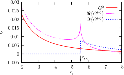
Figure 1: (Color-online) Dependence of the conductance per area of the Kohn-Sham gas in 3D, $G^{0}$, and the real and imaginary parts of the full conductance within the ALDA, ($G^{(b)}$), on the density parameter, $r_{s}$. The ALDA correction is significant within the physically relevant region $2\lesssim r_{s}<r_{s,c}$.

The situation in 3D gas is qualitatively similar. For $q<<q_{F}$ the non-interacting response has the form ($\omega=i\alpha,\alpha>0$)

$$\chi^{0}(q,i\alpha)=-\frac{k_{F}}{\pi^{2}}\left(1-\frac{\alpha}{qk_{F}}\arctan\frac{k_{F}q}{\alpha}\right),$$ (12)

from which, by means of Eqs. (1) and (4), we obtain the conductance per unit area of the Kohn-Sham gas $G^{0}=\frac{k_{F}^{2}}{4\pi^{2}}$. The critical density at which the instability occurs can be found from the appearance of poles of the the irreducible response function in the upper half of the complex plane, which leads to the criterion $B(k_{F,c})\leq-\frac{\pi^{2}}{k_{F,c}}$. The form of the correction to the conductance in 3D cannot be obtained analytically, so we show in Figure 1 our numerical results, which qualitatively resemble the 1D case. We see that the ALDA correction leads to a systematic increase in the conductance. We stress that this correction is a direct consequence of the proper order of limits performed in Eq. 4. From this it also follows that this correction would not be present within the static gDFT calculations based on the NEGF formulation but would appear within a direct time-evolution approach Kurth05 ; Bushong05 if the ALDA is employed. (A minor difference in 3D is that beyond the critical $r_{s,c}$ the formally defined conductance retains a nonzero real part, whereas in 1D it is pure imaginary.)

We briefly discuss a third form of the exchange-correlation kernel, $f_{xc}^{(c)}(q,q^{\prime};\omega)=\frac{\omega^{2}}{q^{2}}C(q,\omega)\delta(q-q^{\prime}),\quad C(q,\omega)\rightarrow C\neq 0$ for $\omega,q\rightarrow 0$. It can be shown that this form of frequency dependence in the kernel also changes the final conductance. This kernel is similar to the one used by Botti et al. Botti05 and Reining et al. Reining02 for bulk insulators and semiconductors characterized by a finite gap in the electronic density of states at the Fermi energy. In their estimate, which lead to significant improvement in the electron energy-loss spectra and optical absorption spectra, the coefficient $C\sim\omega_{g}$ where $\omega_{g}$ is the effective energy gap. This suggests that $f_{xc}^{(c)}=0$ will be zero, or small, in a metallic system.

In order to explore the relevance of these conductance corrections for inhomogeneous systems we consider the metal-vacuum-metal case of two jellium surfaces separated by a distance $d$. In this case the parameter $B$ has been evaluated using Eq. (8) and the Perdew-Zunger Perdew81 parametrization of the quantum Monte Carlo correlation energy of the HEG Ceperley80 . The parameter $A$ is obtained from Eq. (6), and its contribution to the conductance follows from Eq. (5).

In our calculations we employ two jellium slabs of thickness $L$ and density given by $r_{s}$. The calculation of $\chi^{0}(z,z^{\prime};i\alpha)$ is performed at the self-consistent LDA level  Jung04 . Subsequently we invert the Dyson equation, Eq. (4), in real space and thereby calculate the irreducible response $\chi^{irr}(z,z^{\prime};i\alpha)$. For the final step we employ an integral form of Eq. (1)

$$G=-\lim_{\alpha\rightarrow 0^{+}}\alpha\int\frac{dqdq^{\prime}}{2\pi}\frac{\chi^{irr}(q,q^{\prime};i\alpha)}{qq^{\prime}},$$ (13)

where we have used the identity (3). Direct implementation of this expression in reciprocal space is numerically rather cumbersome, since $\chi^{irr}$ is, in practice, calculated for a finite (periodic) supercell for which the region with $q,q^{\prime}<<1$ is poorly described. This problem can be circumvented by re-expressing $G$ in a real-space form,

$$G=-\lim_{\alpha\rightarrow 0^{+}}\alpha\int_{0}^{\infty}dz\int_{-\infty}^{0}dz^{\prime}\chi^{irr}(z,z^{\prime};i\alpha),$$ (14)

which is obtained from (13) by utilizing the fact that the $1/qq^{\prime}$ singularity is only apparent since $\chi(q,q^{\prime})\sim qq^{\prime}$ for small $q,q^{\prime}$. Extrapolation to zero frequency (from $\omega\sim 0.01$ Ha $<<E_{F}$) is done in parallel with extrapolation of the thickness of the slabs $L$ to infinity. Further details of the calculation will be published elsewhere Bokes06 . The quality of the numerical procedure can be judged from the correct exponential decrease in the Kohn-Sham conductance over several orders of magnitude shown in Fig. 2.

The resulting dependence of the conductance on the vacuum width is shown in Fig. 2, for a representative jellium density $r_{s}=3$ a.u. (Au).

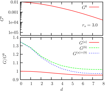
Figure 2: (Color-online) The Kohn-Sham conductance $G^{0}$ (upper panel) and the corrected conductances $G$ (shown relative to $G^{0}$) (lower panel), as a function of the vacuum width $d$. The corrections due to the non-local (a) and ALDA (b) kernels have opposing signs.

For small vacuum widths $d$, the correction due to the ALDA kernel $f_{xc}^{(b)}$ clearly dominates; for larger widths ($d\sim 6-8$ a.u.) $f_{xc}^{(a)}$ and $f_{xc}^{(b)}$ shift the Kohn-Sham conductance in opposite directions and to some extent cancel each other. We should note that unlike the use of a global value for the viscosity in the original work by Sai Sai05 , we have used the local viscosity $\eta[k_{F}(z)]$ in Eq. (6), determined by the local density, which leads to suppression of the non-local corrections for $d\gtrsim 2$a.u.Bokes06

In conclusion, we have presented a unified formalism, based on the singular character of response functions, to address the conductance of a general system of interacting electrons. We have explicitly identified three different contributions to the dynamical resistance: (a) the non-local contribution Sai05 parametrized by the dynamical viscosity of the homogeneous electron gas, effective only for inhomogeneous systems, (b) a local contribution parametrized by the adiabatic LDA exchange-correlation kernel, and (c) an ultra-non-local contribution that, from presently available estimates, is not important for metallic systems. These three forms are unlikely to exhaust all the possibilities, and our theoretical framework remains applicable for further analysis based on many-body perturbation theory to obtain additional relevant contributions to the exchange-correlation kernel or local field factor. In the homogeneous electron gas, we have found that the conductance diverges as the critical density $r_{s,c}$ is approached, beyond which the gas is unstable. For practical calculations, our formalism can readily benefit from available computer codes for ab-initio calculations in real materials that can generate density-density response functions. We have shown the importance of the non-vanishing corrections for the conductance of a model inhomogeneous system.

- (1) J. Taylor, M. Brandbyge, and K. Stokbro, Phys. Rev. Lett. 89, 138301 (2002).
- (2) H. Basch, R. Cohen, and M. A. Ratner, Nano Lett. 5, 1668 (2005).
- (3) N. Sai, M. Zwolak, G. Vignale, and M. DiVentra, Phys. Rev. Lett. 94, 186810 (2005).
- (4) C. Toher, A. Filippetti, S. Sanvito, and K. Burke, Phys. Rev. Lett. 95, 146402 (2005).
- (5) M. Koentopp, K. Burke and F. Evers, Phys. Rev. B 73, 121403(R) (2006).
- (6) J. J. Palacios, Phys. Rev. B 72, 125424 (2005).
- (7) G. Stefanucci and C. O. Almbladh, Phys. Rev. B 69, 195318 (2004).
- (8) M. D. Ventra and T. N. Todorov, J. Phys.: Condens. Matter 16, 8025 (2004).
- (9) G. Vignale, C. A. Ullrich, and S. Conti, Phys. Rev. Lett. 79, 4878 (1997).
- (10) A. Ferretti et al., Phys. Rev. Lett. 94, 116802 (2005).
- (11) P. Delaney and J. C. Greer, Phys. Rev. Lett. 93, 036805 (2004).
- (12) P. Bokes and R. W. Godby, Phys. Rev. B 69, 245420 (2004).
- (13) D. Pines and P. Nozieres, The Theory of Quantum Liquids (W. A. Benjamin, Inc., New York, 1966).
- (14) P. Bokes, J. Jung, and R. W. Godby, (to be published) (2006).
- (15) G. Vignale and W. Kohn, Phys. Rev. Lett. 77, 2037 (1996).
- (16) E. K. U. Gross and W. Kohn, Phys. Rev. Lett. 55, 2850 (1985).
- (17) S. Kurth et al., Phys. Rev. B 72, 035308 (2005).
- (18) N. Bushong, N. Sai, and M. D. Ventra, Nano Lett. 5, 2569 (2005).
- (19) S. Botti et al., Phys. Rev. B 72, 125203 (2005).
- (20) L. Reining, V. Olevano, A. Rubio, and G. Onida, Phys. Rev. Lett. 88, 66404 (2002).
- (21) J. P. Perdew and A. Zunger, Phys. Rev. B 23, 5048 (1981).
- (22) D. M. Ceperley and B. J. Alder, Phys. Rev. Lett. 45, 566 (1980).
- (23) J. Jung, P. Garcia-Gonzalez, J. F. Dobson, and R. W. Godby, Phys. Rev. B 70, 205107 (2004).