On the generation of multipartite entangled states in Josephson architectures

Abstract

We propose and analyze a scheme for the generation of multipartite entangled states in a system of inductively coupled Josephson flux qubits. The qubits have fixed eigenfrequencies during the whole process in order to minimize decoherence effects and their inductive coupling can be turned on and off at will by tuning an external control flux. Within this framework, we will show that a W state in a system of three or more qubits can be generated by exploiting the sequential one by one coupling of the qubits with one of them playing the role of an entanglement mediator.

I Introduction

Entanglement “the striking feature of quantum mechanics” (as claimed by E. Schrödinger in 1935 schro ) has been considered essential since the very beginning in order to investigate fundamental aspects of quantum theory. Quite recently, however, physicists have fully recognized that the generation of entangled states is an essential resource also in quantum communication and information processing. Entangled states have been generated in many experiments involving cavity QED and NMR systems, ion traps, and solid-state (superconducting) circuits, and their applications in the field of quantum computing have been demonstrated.cavity ; multiqubit ; dot ; ions ; zanardi Among the previously mentioned physical systems, Josephson-junction based devices presently provide one of the best qubit candidates for the realization of a quantum computer due to the fact that a wide variety of potential designs for qubits and their couplings are available and that qubits can be easily scaled to large arrays and integrated in electronic circuits.makhlin ; noritoday A series of successfully performed experiments for charge, flux, phase, and charge-flux qubits show indeed that they satisfy DiVincenzo’s prescriptions divincenzo for quantum computing in terms of state preparation, state manipulation, and readout. Moreover, the nonlinearity characterizing Josephson junctions and the flexibility in circuit layout offer many possible options for coupling qubits together and for calibrating and adjusting the qubit parameters over a wide range of values.

In this field, remarkable achievements include the realization of complex single-qubit manipulation schemes,[3] the generation of entangled states [4] ; [5] in systems of coupled flux [3a] and phase [4a] ; [5a] qubits, as well as the observation of quantum coherent oscillations and conditional gate operations using two coupled superconducting charge qubits.[2] ; [4] The next major step toward building a Josephson-junction based quantum computer is therefore to experimentally realize simple quantum algorithms, such as the creation of an entangled state involving more than two coupled qubits.zanardi ; multiqubit ; w ; cirac ; yuasa

This goal may be achieved by selectively turning on and off the direct couplings between two qubits or their interaction with auxiliary systems ($LC$-oscillator modes,buisson inductances,nori large-area current-biased Josephson junctions,martinis ; wei or the quantized modes of a resonant microwave cavity noi-prb ; girvin ; frunzio ) playing the role of a data bus. Typically, the coupling energy may be controlled by tuning the qubit level spacings in and out of resonance. However, in order to avoid introducing extra decoherence with respect to that characterizing single-qubit operations, other promising scheme for realizing a tunable coupling of superconducting (spatially separated) qubits have emerged: for instance that wherein the interaction between two flux-based qubits is controlled by means of a superconducting transformer with variable flux transfer function,cosmellitransf or those wherein two qubits with an initial detuning can be made to (resonantly) interact by applying a time-dependent (microwave) magnetic flux to the qubits.norideph

Within these experimental frameworks, we propose a theoretical scheme by which it is possible to entangle more than two (spatially separated) flux qubits. It is based on the sequential inductive interaction of the qubits with one of them acting as an entanglement mediator.mediator ; Haroche More in detail, we will see that the scheme operates in such a way that it generates an entangled W state after a finite number of steps, that no conditional measurement is required, and that the proposed architectures are scalable, at least in principle, to an arbitrary number of qubits.

The paper is organized as follows. First, in Sec. II, we briefly describe the main features and the Hamiltonians characterizing two kinds of Josephson devices, namely the double rf-SQUID luk ; cosm ; chiarello and the persistent (three-junction) SQUID,mooij99 by which it is possible to build superconducting flux qubits. Then, we discuss the most common experimental procedures by which it is possible to initialize and to measure their quantum state. In Sec. III, a scheme of successive interaction is introduced in an ($N+1$)-qubit system, qubit M+qubit 1+$\cdots$+qubit $N$, wherein entanglement mediator M is coupled one by one with qubits 1, 2, …, $N$. We discuss moreover the possibility of practically realizing this scheme by exploiting some of the different physical coupling elements currently available and how the coupling energy depends on the particular way in which the interaction between each qubit and the mediator is implemented. In Sec. IV, we analyze the dynamics of the system showing that, by preparing the multi-qubit system in a pure factorized state and by adjusting the coupling energies and/or the time of interaction between each of them and the mediator, an entangled W state can be generated. Finally, conclusions and discussions are given in Sec. V.

II Superconducting Flux Qubits: Models and Hamiltonians

In this section, we briefly describe the main features and the Hamiltonians of two devices, the tunable rf-SQUID luk ; cosm ; chiarello and the three-junction SQUID,mooij99 by which it is possible to implement a two-state Josephson system, focusing our attention also on the experimental procedures to be considered in order to prepare their initial quantum state.

II.1 The double rf-SQUID qubit

We begin by considering a double rf-SQUID system,luk ; cosm ; chiarello that is a superconducting ring of self-inductance $L$ interrupted by a dc-SQUID, a smallest loop containing two identical Josephson junctions, each with critical current $i_{0}$ and capacitance $c$. This device [schematically illustrated in Fig. 1(a)] is biased by two magnetic fluxes $\phi_{x}$ and $\phi_{c}$ threading the greatest ring and the dc-SQUID, respectively.

The dc-SQUID if small enough (i.e. with inductance $l\ll i_{0}\phi_{0}/2\pi$, where $\phi_{0}=h/2e$ is the flux quantum) behaves like a single junction with a flux-dependent critical current $I_{c}=2i_{0}|\cos(\pi\phi_{c}/\phi_{0})|$ and capacitance $C=2c$. This means that a double SQUID simulates a standard rf-SQUID with tunable critical current $I_{c}\equiv I_{c}(\phi_{c})$.

Therefore, by taking into account both the charging energy of the “effective dc-SQUID junction” ($T=q^{2}/2C$) and the washboard potential, the Hamiltonian of the system is written down as

$$H=\frac{q^{2}}{2C}+\frac{(\phi-\phi_{x})^{2}}{2L}-\frac{I_{c}\phi_{0}}{2\pi}\cos\!\left(\frac{2\pi\phi}{\phi_{0}}\right),$$ (1)

where the charge on the junction capacitance, $q$, and the flux through the SQUID loop, $\phi$, are canonically conjugate operators satisfying the commutation relation $[\phi,q]=i\hbar$.

It is well known chiarello ; chiarello2 that, by setting $\beta_{L}\equiv 2\pi LI_{c}/\phi_{0}>1$ and $\phi_{x}\approx\phi_{0}/2$, the circuit behaves as an artificial quantum two-level atom whose reduced Hamiltonian in the basis of the flux eigenstates $|{L}\rangle$ and $|{R}\rangle$ (which are localized in the two minima of the washboard potential and correspond to two different orientations of the current circulating in the large loop) assumes the form

$$H_{\text{RF}}=-\frac{\hbar}{2}\Delta_{\text{RF}}(\phi_{c})\sigma_{x}-\frac{\hbar}{2}\epsilon_{\text{RF}}(\phi_{x})\sigma_{z}.$$ (2)

Here, $\hbar\epsilon_{\text{RF}}(\phi_{x})=2I_{c}\sqrt{6(\beta_{L}-1)}(\phi_{x}-\phi_{0}/2)$ is the energy difference between the two minima of the washboard potential,

$$\Delta_{\text{RF}}(\phi_{c})\simeq\frac{3}{2}\frac{\phi_{0}^{2}}{(2\pi)^{2}L}\left(1-\frac{\phi_{0}}{2\pi LI_{c}(\phi_{c})}\right)^{2}$$ (3)

(in the limit $0<\beta_{L}-1\ll 1$) the tunnelling frequency between the left and the right wells that can be tuned by changing the junction critical current $I_{c}(\phi_{c})$, and $\sigma_{x}$ and $\sigma_{z}$ the Pauli spin operators.

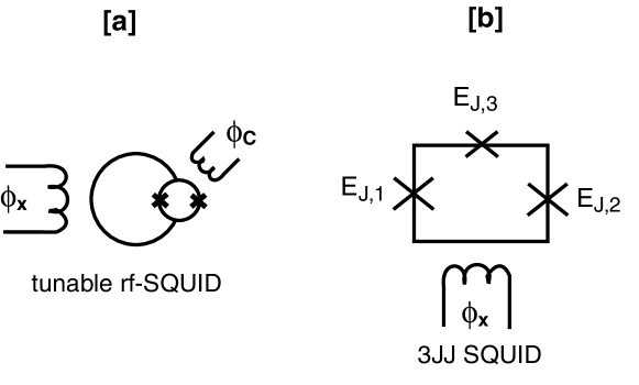
Figure 1: Sketch (a) of the superconducting double rf-SQUID qubit and (b) of the three-junction SQUID by which it is possible to realize a persistent-current qubit.

II.2 The persistent-current (3JJ) qubit

To minimize the susceptibility to external noise of a large-inductance rf-SQUID, Mooij et al.mooij99 proposed to use a persistent-current qubit [schematically shown in Fig. 1(b)], namely a smaller superconducting loop containing three Josephson junctions, two of equal size (i.e. with $E_{J,1}=E_{J,2}=E_{J}$) and the third smaller by a factor $\alpha$ (i.e. with $E_{J,3}=\alpha E_{J}$, $\alpha<1$). By applying an external magnetic flux $\phi_{x}$ close to $\phi_{0}/2$ and choosing $\alpha\approx 0.8$, it has been proved that, in the low-inductance limit (in which the total flux coincides with the external flux and fluxoid quantization around the loop imposes the constraint $\varphi_{1}-\varphi_{2}+\varphi_{3}+2\pi f=0$ on the phase drops across the three junctions, $f=\phi_{x}/\phi_{0}$ being the reduced magnet flux), the Josephson energy

$$U(\varphi_{1},\varphi_{2})=-E_{J}\cos\varphi_{1}-E_{J}\cos\varphi_{2}-\alpha E_{J}\cos(2\pi f+\varphi_{1}-\varphi_{2})$$ (4)

forms a double well which permits two stable configurations of minimum energy corresponding to two persistent currents of opposite sign in the loop. This means that, also in this case, we may engineer a two-state quantum system whose effective Hamiltonian, in the basis of the two states that carry an average persistent current $\pm I_{p}\approx\pm 2\pi\alpha E_{J}/\phi_{0}$ (named $|{L}\rangle$ and $|{R}\rangle$ also in this case), reads

$$H_{\text{3JJ}}=-\frac{\hbar}{2}\Delta_{\text{3JJ}}\sigma_{x}-\frac{\hbar}{2}\epsilon_{\text{3JJ}}(\phi_{x})\sigma_{z}.$$ (5)

Here, the tunnelling matrix element between the two basis states, $\hbar\Delta_{\text{3JJ}}/2$, depends on the system parameters, and $\epsilon_{\text{3JJ}}(\phi_{x})=2I_{p}(\phi_{x}-\phi_{0}/2)/\hbar$.

II.3 Initialization and readout

Using as a new basis that is spanned by the energy eigenstates $|{0}\rangle$ and $|{1}\rangle$ (which are the symmetric and the antisymmetric linear superpositions of $|{L}\rangle$ and $|{R}\rangle$, if $\phi_{x}$ is exactly equal to $\phi_{0}/2$), the Hamiltonians of both the rf-SQUID qubit and the 3JJ qubit take the diagonal spin $1/2$-like form

$$H=\frac{\hbar}{2}\omega\sigma_{z}.$$ (6)

Here, $\hbar\omega\equiv E_{1}-E_{0}=\hbar\sqrt{\epsilon^{2}+\Delta^{2}}$ indicates the energy separation between their corresponding eigenstates (the analytic form of $\epsilon$ and $\Delta$, as previously discussed, depends on the specific design of the qubit) and $\sigma_{z}=|{1}\rangle\langle{1}|-|{0}\rangle\langle{0}|$ is a Pauli operator.

Before discussing the modus operandi of our scheme, it is worth noting that both the rf-SQUID qubit and the 3JJ qubit are easily addressed and measured. Usually, they are initialized to the ground state simply by allowing them to relax, so that the thermal population of their excited states can be neglected. The coherent control of the qubit state is instead achieved via NMR-like manipulation techniques, i.e. by applying resonant microwave pulses which, by opportunely choosing the interaction time and the microwave amplitude, can induce a transition between the two qubit energy levels.[3]

In addition, a flux state can be prepared producing a collapse of the wave function through a flux measurement or, as recently pointed out by Chiarello,chiarello2 in the case of a double rf-SQUID qubit with an opportunely chosen sequence of variations of the washboard potential. A double SQUID can be indeed prepared in a particular flux state by strongly unbalancing the washboard potential in order to have just one minimum, then waiting a time sufficient for the relaxation to this minimum and finally sufficiently raising the barrier in order to freeze the qubit in this state. Finally, coherent rotation between the two flux states can be realized by lowering the barrier in order to induce fast free oscillations, waiting for fractions of the oscillation period to realize the desired rotation and opportunely raising the barrier in such a way to freeze the system in the desired target state.

Also for qubit readout, several detectors have been experimentally investigated. Most of them include a dc-SQUID magnetometer inductively coupled to the qubit to be measured by which it is possible to detect the magnetization signal produced by the persistent currents flowing through it, exploiting the fact that the dc-SQUID critical current is a periodic function of the magnetic flux threading its loop.cosm In addition, it is worth emphasizing that, besides these proposals, physicists have been focusing their efforts on the realization of nondemolition-measurement schemes (necessary for applications where low back-action is required) like that based on the dispersive measurement of the qubit state by coupling the qubit nonresonantly to a transmission-line resonator and probing the transmission spectrum.readout

III The Scheme for Entanglement Generation: Sequential Interaction of $N$ Flux Qubits with an Entanglement Mediator

In this section, we propose a scheme for the generation of maximally entangled states in a multi-qubit system, $\text{M}+1+2+\cdots+N$, where qubit M, playing the role of an entanglement mediator, is assumed to interact one by one with $1$, $2$, …, and $N$. Among the different forms of coupling theoretically proposed and experimentally realized, we consider those by which it is possible to realize an inductive interaction cosmellitransf ; norideph ; plourde between each qubit and the mediator, so that the free Hamiltonian of the whole system and the interaction Hamiltonians can be cast (in the basis of the energy eigenstates) in the following form:

$$H_{0}=\sum_{i=M,1,2,\ldots,N}\frac{\hbar}{2}\omega_{i}\sigma_{z}^{(i)}$$ (7)

and

$$H_{M1}^{\prime}=g_{1}\sigma_{x}^{(M)}\sigma_{x}^{(1)},\quad H_{M2}^{\prime}=g_{2}\sigma_{x}^{(M)}\sigma_{x}^{(2)},\quad\ldots,\quad H_{MN}^{\prime}=g_{N}\sigma_{x}^{(M)}\sigma_{x}^{(N)}.$$ (8)

We assume moreover that these qubits are properly initialized, by exploiting one of the previously mentioned experimental recipes, so that at $t=0$ the whole system is described by the pure factorized state $|{1_{M}0_{1}0_{2}\ldots 0_{N}}\rangle\equiv|{1}\rangle_{M}\otimes|{0}\rangle_{1}\otimes|{0}\rangle_{2}\otimes\cdots\otimes|{0}\rangle_{N}$.

With this setup, if qubits $1$, $2$, …, and $N$ are spatially separated (in order to strongly reduce their direct persistent coupling) and their interaction with mediator M can be turned on and off at will (by adjusting the coupling energies $g_{1}$, $g_{2}$, …, $g_{N}$), we realize a step by step scheme which is sketched as follows:

• Mediator M prepared in the state $|{1}\rangle_{M}$ interacts inductively (by setting $g_{1}\neq 0$) with qubit $1$ during an opportunely chosen interval of time $0<t<\tau_{1}$, while qubits $2$, $3$, …, and $N$ evolve freely (with $g_{2}=g_{3}=\cdots=g_{N}=0$).

• At $t=\tau_{1}$, we turn off the interaction between M and $1$ and we adjust $g_{2}$ in order to couple the mediator and qubit $2$ (by choosing $g_{2}\neq 0$) for $\tau_{1}<t<\tau_{1}+\tau_{2}$.

• In a similar manner, we put qubits $3$, $4$, …, and $N$ in interaction with M one by one.

• Finally, at $t=\tau_{1}+\tau_{2}+\cdots+\tau_{N}$, we switch off the interaction between qubit $N$ and mediator M, and the desired entangled state of the $(N+1)$-partite qubit M+qubit 1+$\cdots$+qubit $N$ system is generated, provided that the interaction times, $\tau_{j}$ (with $j=1,2,\ldots,N$), and/or the coupling constants, $g_{j}$, are accurately selected.

At this stage, it is important to consider a realistic experimental setup by which it is possible to implement our scheme. We begin by considering an inductive mediator-qubit coupling realized by means of a superconducting transformer with variable flux transfer function as in the paper of Cosmelli et al.cosmellitransf They show indeed that, by using a superconducting flux transformer modified with the insertion of a small dc-SQUID, it is possible to control the flux transfer function and therefore the inductive coupling constant, by modulating via an externally applied magnetic flux $\phi_{cx}$ the critical current of the dc-SQUID (see Fig. 2). More in detail, they prove that the transformer can operate between two states with very different behavior: the “off” state where the transfer ratio $\mathcal{R}=\phi_{\text{out}}/\phi_{\text{in}}$ is minimum ($\sim 0$–$0.1$) and the “on” state with a transfer function ratio which may be also larger than 1. Under such conditions, it is possible to conceive an experimental scheme, like that depicted in Fig. 3, where the coupling between mediator M and the $j$th qubit may be effectively turned on by adjusting the control fluxes of the relative “switches” in such a way that one obtains $g_{j}\neq 0$ with all the other “switches” kept in the off state.

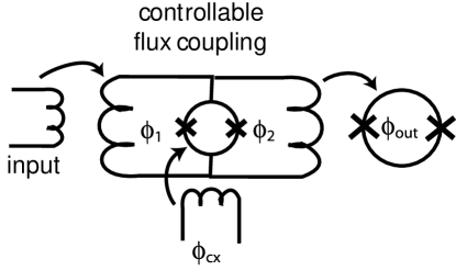
Figure 2: Sketch of a controllable flux coupling (CFC) circuit. A signal flux is applied on the left side of the CFC and its response is read out/coupled to the SQUID on the right. The control of the transmitted flux $\phi_{\text{out}}$ is achieved by modulating the flux $\phi_{cx}$.cosmellitransf

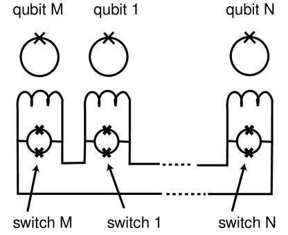
Figure 3: Sketch of the scheme for the controlled coupling of more flux qubits proposed by Cosmelli et al.cosmellitransf

Similarly, Plourde et al. propose to adjust the coupling strength characterizing the interaction between two 3JJ flux qubits by changing the critical current of a dc-SQUID (which is coupled to each of these two qubits), finding that their coupling constant can be changed continuously from positive to negative values (and enables cancellation of the direct mutual inductive coupling if the two qubits are not spatially separated).plourde

Adopting one of these experimental coupling setups, it is therefore possible to realize the step by step scheme in the system of $N+1$ qubits whose Hamiltonian during each of the aforementioned steps assumes the following form:

$$H_{Mj}=H_{0}+H_{Mj}^{\prime}=H_{M}+H_{1}+H_{2}+\cdots+H_{N}+H_{Mj}^{\prime}\quad(j=1,2,\ldots,N).$$ (9)

We observe that the structure of the multipartite Hamiltonian during each step allows us to simplify the study of its dynamics by confining ourselves to the analysis of the dynamics of the bipartite mediator-SQUID-$1$ system during the time interval $0<t<\tau_{1}$, to that of the mediator-SQUID-$2$ system during the second period $\tau_{1}<t<\tau_{1}+\tau_{2}$, and so on (of course, provided that the free evolution of the other qubits is carefully taken into account).

Moreover, by assuming that all the qubits and entanglement mediator M have a common energy gap $\omega=\omega_{i}$, $\forall\;i\equiv\{M,1,2,\ldots,N\}$, due to the preponderance of rotating-wave terms of the interaction Hamiltonians with respect to the counter-rotating ones, it is not difficult to convince oneself that, during each step, the system dynamics is dominated by the bipartite Hamiltonian

$$H_{Mj}^{\text{RWA}}=H_{M}+H_{j}+H_{Mj}^{\text{RWA}\prime}=\frac{\hbar}{2}\omega_{M}\sigma_{z}^{(M)}+\frac{\hbar}{2}\omega_{j}\sigma_{z}^{(j)}+g_{j}(\sigma_{+}^{(M)}\sigma_{-}^{(j)}+\sigma_{-}^{(M)}\sigma_{+}^{(j)}),\qquad\omega_{M}=\omega_{j}=\omega,$$ (10)

describing the rotating-wave coupling between the mediator and the $j$th qubit. In the following section, we will demonstrate the validity of this assumption. It is interesting, however, to note that Hamiltonian (10) can be exactly implemented if the detuning $\Delta=\omega_{M}-\omega_{j}$ between the two flux (3JJ) qubits to be coupled is chosen sufficiently large so that initially each of them can be treated independently. As recently shown by Liu et al.,norideph in fact, this gap can be nullified by applying to one of the two SQUID loops a time dependent magnetic flux $\phi_{x}^{(\ell)}(t)=A_{\ell}\cos\omega_{c}^{(\ell)}t$ (with $\ell=M$ or $j$) satisfying the condition $\Delta\pm\omega_{c}^{(\ell)}=0$ when $\Delta\lessgtr 0$. This means that, by considering the reduced bias flux of each qubit close to $\phi_{0}/2$ and the aforementioned frequency-matching condition, it is possible to implement the interaction Hamiltonian $H_{Mj}^{\text{int}}=g_{j}(\sigma_{+}^{(M)}\sigma_{-}^{(j)}+\sigma_{-}^{(M)}\sigma_{+}^{(j)})$, where $g_{j}$ can be controlled for instance by tuning the amplitude $A_{\ell}$ of the applied time-dependent magnetic flux.

IV W-State Generation

Now, we analyze the dynamics of the system and demonstrate that the scheme introduced in the previous section actually generates an entangled W state of a tripartite system. We show further that it can be extended to the case of a larger number of qubits.

We begin our analysis by looking at the eigensolutions of Hamiltonian (10), which is represented in the basis $\{|{01}\rangle_{Mj},|{10}\rangle_{Mj},|{00}\rangle_{Mj},|{11}\rangle_{Mj}\}$ by the following simple diagonal block form:

$$H_{Mj}^{\text{RWA}}=\left(\begin{array}[]{c c c c}0&g_{j}&0&0\\ g_{j}&0&0&0\\ 0&0&-\hbar\omega&0\\ 0&0&0&\hbar\omega\end{array}\right).$$ (11)

These blocks describe three dynamically separate subspaces: the first with characteristic frequency $g_{j}/\hbar$ characterizing the appearance of the entanglement between the degenerate states $|{01}\rangle_{Mj}$ and $|{10}\rangle_{Mj}$, and the other ones describing the fact that the two states $|{00}\rangle_{Mj}$ and $|{11}\rangle_{Mj}$ evolve freely. We easily find that the eigenstates of $H_{Mj}^{\text{RWA}}$ are

$$|{u_{1j}}\rangle=\frac{1}{\sqrt{2}}[|{10}\rangle_{Mj}-|{01}\rangle_{Mj}],\quad|{u_{2j}}\rangle=\frac{1}{\sqrt{2}}[|{10}\rangle_{Mj}+|{01}\rangle_{Mj}],\quad|{u_{3j}}\rangle=|{00}\rangle_{Mj},\quad|{u_{4j}}\rangle=|{11}\rangle_{Mj},$$ (12)

with eigenvalues

$$\lambda_{1j/2j}=\mp g_{j},\qquad\lambda_{3j/4j}=\mp\hbar\omega.$$ (13)

IV.1 Generation of entangled W states of the tripartite “M+1+2” system

By exploiting the knowledge of the eigensolutions of Hamiltonian $H_{Mj}^{\text{RWA}}$, it is possible to follow step by step the dynamics of the three-qubit system characterized by the one by one interaction of mediator M with qubits 1 and 2. We choose as an initial condition the state

$$|{1_{M}0_{1}0_{2}}\rangle.$$ (14)

During the first step, we switch on the interaction between M and 1 and we let them interact for a time $\tau_{1}$, while 2 evolves freely. This process generates the state

$$e^{-iH_{M1}\tau_{1}/\hbar}|{1_{M}0_{1}0_{2}}\rangle=e^{-i(H_{0}+H_{M1}^{\text{RWA}}{}^{\prime})\tau_{1}/\hbar}|{1_{M}0_{1}0_{2}}\rangle=e^{i\omega\tau_{1}/2}[\cos\theta_{1}|{1_{M}0_{1}0_{2}}\rangle-i\sin\theta_{1}|{0_{M}1_{1}0_{2}}\rangle],$$ (15)

where $\theta_{1}\equiv g_{1}\tau_{1}/\hbar$. Next, by turning on the interaction between M and 2 at $t=\tau_{1}$ and by allowing qubit 1 evolves freely during the second step (i.e. during the interval of time $\tau_{1}<t<\tau_{1}+\tau_{2}$), we obtain:

$$|{\varphi_{2}}\rangle =e^{-iH_{M2}\tau_{2}/\hbar}e^{-iH_{M1}\tau_{1}/\hbar}|{1_{M}0_{1}0_{2}}\rangle$$

$$=e^{i\omega(\tau_{1}+\tau_{2})/2}[\cos\theta_{1}\cos\theta_{2}|{1_{M}0_{1}0_{2}}\rangle-i\sin\theta_{1}|{0_{M}1_{1}0_{2}}\rangle-i\cos\theta_{1}\sin\theta_{2}|{0_{M}0_{1}1_{2}}\rangle].$$ (16)

Equation (16) clearly shows that, by adjusting $\theta_{j}\equiv g_{j}\tau_{j}/\hbar$ ($j=1,2$) so that

$$|\sin\theta_{1}|=\frac{1}{\sqrt{3}}\quad\text{and}\quad|\cos\theta_{2}|=\frac{1}{\sqrt{2}},$$ (17)

a tripartite W state is generated. If we choose $\theta_{2}=\pi/4$ and $\theta_{1}$ such that $\sin\theta_{1}=1/\sqrt{3}$ and $\cos\theta_{1}=\sqrt{2/3}$, for instance, we get

$$|{W_{2}}\rangle=\frac{1}{\sqrt{3}}e^{i\omega(\tau_{1}+\tau_{2})/2}[|{1_{M}0_{1}0_{2}}\rangle-i|{0_{M}1_{1}0_{2}}\rangle-i|{0_{M}0_{1}1_{2}}\rangle].$$ (18)

It is worth noting that we obtain this state by adjusting the coupling energies $g_{j}$ during the aforementioned steps and/or by tuning the interaction times $\tau_{j}$.

IV.2 Generation of entangled W states of the multipartite “M+1+2+$\cdots$+$N$” system

Within this framework, it is possible to look at the possibility of applying the same techniques in order to generate an entangled state of a multipartite “M+1+2+$\cdots$+$N$” system with $N>2$. As described in Sec. III, we consider an entanglement mediator M in interaction one by one with $N$ qubits. If the system is prepared at $t=0$ in the factorized state

$$|{1_{M}0_{1}0_{2}\ldots 0_{N}}\rangle,$$ (19)

after a straightforward approach it is easy to show that at the end of the $N$th step (namely at $t=t_{N}\equiv\sum_{j=1}^{N}\tau_{j}$) it can be described in terms of the state

$$|{\varphi_{N}}\rangle=e^{i(N-1)\omega t_{N}/2}[\cos\theta_{1}\cos\theta_{2}\cdots\cos\theta_{N}|{1_{M}0_{1}0_{2}\ldots 0_{N}}\rangle\\ -i\sin\theta_{1}|{0_{M}1_{1}0_{2}\ldots 0_{N}}\rangle-\cdots-i\cos\theta_{1}\cos\theta_{2}\cdots\cos\theta_{k-1}\sin\theta_{k}|{0_{M}0_{1}0_{2}\ldots 1_{k}\ldots 0_{N}}\rangle\\ -\cdots-i\cos\theta_{1}\cos\theta_{2}\cdots\cos\theta_{N-1}\sin\theta_{N}|{0_{M}0_{1}0_{2}\ldots 1_{N}}\rangle].$$ (20)

Assuming that it is possible to control the interaction time $\tau_{j}$ of each qubit with mediator M and/or their coupling constants $g_{j}$ so that

$$\sin\theta_{j}=\frac{1}{\sqrt{N-j+2}}\quad\text{and}\quad\cos\theta_{j}=\sqrt{\frac{N-j+1}{N-j+2}},$$ (21)

we finally find that the generalized W entangled state

$$|{W_{N}}\rangle=\frac{e^{i(N-1)\omega t_{N}/2}}{\sqrt{N+1}}[|{1_{M}0_{1}0_{2}\ldots 0_{N}}\rangle-i|{0_{M}1_{1}0_{2}\ldots 0_{N}}\rangle-i|{0_{M}0_{1}1_{2}\ldots 0_{N}}\rangle\cdots-i|{0_{M}0_{1}0_{2}\ldots 1_{N}}\rangle]$$ (22)

of the $(N+1)$-partite system is created.

IV.3 Estimation of the effect of counter-rotating terms

At this stage, we wish to test the validity of the rotating-wave approximation (RWA) performed at the end of Sec. III. To this end, we analyze the fidelity of the system state $|{\psi_{N}}\rangle$ calculated without performing the RWA on the Hamiltonian model with respect to the target state (22), i.e. $\mathcal{F}_{N}=|\langle{W_{N}}|{\psi_{N}}\rangle|$.

Let us first look at the fidelity for the tripartite W state. After a straightforward calculation, we find that, by following the aforementioned two-step procedure, the $\sigma_{x}^{(M)}\sigma_{x}^{(j)}$ couplings generate the state

$$|{\psi_{2}}\rangle=\frac{1}{\sqrt{3}}e^{i\omega(\tau_{1}+\tau_{2})/2}\left\{|{1_{M}0_{1}0_{2}}\rangle-i|{0_{M}0_{1}1_{2}}\rangle-ie^{-i\omega\tau_{2}}\left[\left(\cos\chi_{2}+i\frac{\hbar\omega}{\sqrt{g_{2}^{2}+\hbar^{2}\omega^{2}}}\sin\chi_{2}\right)|{0_{M}1_{1}0_{2}}\rangle\right.\right.\\ \left.\left.-i\frac{g_{2}}{\sqrt{g_{2}^{2}+\hbar^{2}\omega^{2}}}\sin\chi_{2}|{1_{M}1_{1}1_{2}}\rangle\right]\right\}$$ (23)

with the same $\theta_{1}$ as that for (18), where $\chi_{2}=\sqrt{g_{2}^{2}/\hbar^{2}+\omega^{2}}\tau_{2}$. Its fidelity $\mathcal{F}_{2}=0.999957$, calculated with $g_{2}/\hbar\approx 0.5\,\text{GHz}$, $\omega\approx 10\,\text{GHz}$ (in agreement with the currently available experimental values), confirms that during each step the system dynamics is dominated by the bipartite Hamiltonian (10) describing the rotating-wave coupling between the mediator and the $j$th qubit.

For the ($N+1$)-partite system, the generated state reads

$$|{\psi_{N}}\rangle=\frac{e^{i(N-1)\omega t_{N}/2}}{\sqrt{N+1}}\,\Biggl{[}|{1_{M}0_{1}0_{2}\ldots 0_{N}}\rangle-i|{0_{M}0_{1}0_{2}\ldots 1_{N}}\rangle\\ -i\sum_{k=1}^{N-1}\left\{\prod_{j=k+1}^{N}e^{-i\omega\tau_{j}}\left(\cos\chi_{j}+i\frac{\hbar\omega}{\sqrt{g_{j}^{2}+\hbar^{2}\omega^{2}}}\sin\chi_{j}\right)\right\}|{0_{M}0_{1}0_{2}\ldots 1_{k}\ldots 0_{N}}\rangle\\ +\text{(states orthogonal to $|{W_{N}}\rangle$)}\Biggr{]}$$ (24)

with the tuning (21), where $\chi_{j}=\sqrt{g_{j}^{2}/\hbar^{2}+\omega^{2}}\tau_{j}$, and the fidelity is given by

$$\mathcal{F}_{N}=\frac{1}{N+1}\left|2+\sum_{k=1}^{N-1}\prod_{j=k+1}^{N}e^{-i\omega\tau_{j}}\left(\cos\chi_{j}+i\frac{\hbar\omega}{\sqrt{g_{j}^{2}+\hbar^{2}\omega^{2}}}\sin\chi_{j}\right)\right|,$$ (25)

which results in

$$\mathcal{F}_{3}=0.999873,\quad\mathcal{F}_{4}=0.999601,\quad\ldots,\quad\mathcal{F}_{10}=0.997561,\quad\ldots,\quad\mathcal{F}_{20}=0.993959,\quad\text{etc.}$$ (26)

when $g_{1}/\hbar=\cdots=g_{N}/\hbar\approx 0.5\,\text{GHz}$ and $\omega\approx 10\,\text{GHz}$. The physical meaning of such a list of values is that we might implement our scheme using up to $20$ qubits maintaining a very good level of fidelity of the state given by Eq. (24) with respect to the target state expressed by Eq. (22).

V Conclusions

In this paper, we have discussed a scheme for the generation of entangled W states among three Josephson (eventually spatially separated) flux qubits as well as its generalization to the case of $N+1$ qubits. The success of the scheme relies on the possibility of realizing controllable couplings between the qubits and entanglement mediator M and on the possibility of preparing their initial quantum state. It should be stressed that no conditional measurement are required but we have to tune the coupling energy and/or the interaction time between each qubit and the mediator.

Final considerations are devoted to the analysis of some aspects of decoherence problem in our system. In particular, we wish to verify if the operation duration (e.g. the time necessary to perform the desired quantum process) is small enough with respect to the decoherence time. We find, on the one hand, that the eigenfrequency of a Josephson qubit $\omega$ is of the order of $10\,\text{GHz}$ and that correspondingly $g_{j}/\hbar\approx 0.5\,\text{GHz}$. Under such conditions, the length of each step (during which only a fraction of a Rabi oscillation takes place) is at most of the order of $\hbar/g_{j}\approx 2\,\text{ns}$ and consequently the whole process in the case, for instance, of a tripartite system lasts approximatively $4\,\text{ns}$. On the other hand the relaxation and decoherence times, $T_{1}$ and $T_{2}$, of a superconducting flux qubit have been coarsely estimated and are in the range $1$–$10\,\mu\text{s}$.noritoday ; cosmel Therefore this means that a number of operations can be performed before decoherence occurs and that, in principle, our quantum information processing can be exploited for the experimental generation of entangled W states among more than three qubits.

- (1) E. Schrödinger, Naturwissenschaften 23, 807 (1935); 23, 823 (1935); 23, 844 (1935); reprinted in English in Quantum Theory and Measurement, edited by J. A. Wheeler and W. H. Zurek (Princeton University Press, New Jersey, 1984).
- (2) L. Ye, L.-B. Yu, and G.-C. Guo, Phys. Rev. A 72, 034304 (2005).
- (3) X. Wang, M. Feng, and B. C. Sanders, Phys. Rev. A 67, 022302 (2003).
- (4) A. Barenco, D. Deutsch, A. Ekert, and R. Jozsa, Phys. Rev. Lett. 74, 4083 (1995); D. Loss and D. P. DiVincenzo, Phys. Rev. A 57, 120 (1998); T. Tanamoto, ibid. 61, 022305 (2000); E. Biolatti, R. C. Iotti, P. Zanardi, and F. Rossi, Phys. Rev. Lett. 85, 5647 (2000); X.-Q. Li and Y. J. Yan, Phys. Rev. B 65, 205301 (2002).
- (5) J. J. García-Ripoll, P. Zoller, and J. I. Cirac, Phys. Rev. A 71, 062309 (2005); P. C. Haljan, P. J. Lee, K.-A. Brickman, M. Acton, L. Deslauriers, and C. Monroe, ibid. 72, 062316 (2005).
- (6) S.-L. Zhu, Z. D. Wang, and P. Zanardi, Phys. Rev. Lett. 94, 100502 (2005).
- (7) Y. Makhlin, G. Schön, and A. Shnirman, Rev. Mod. Phys. 73, 357 (2001).
- (8) J. Q. You and F. Nori, Phys. Today 58, 42 (2005).
- (9) D. P. DiVincenzo, Fortschr. Phys. 48, 771 (2000).
- (10) E. Collin, G. Ithier, A. Aassime, P. Joyez, D. Vion, and D. Esteve, Phys. Rev. Lett. 93, 157005 (2004).
- (11) T. Yamamoto, Yu. A. Pashkin, O. Astafiev, Y. Nakamura, and J. S. Tsai, Nature (London) 425, 941 (2003).
- (12) R. McDermott, R. W. Simmonds, M. Steffen, K. B. Cooper, K. Cicak, K. D. Osborn, S. Oh, D. P. Pappas, and J. M. Martinis, Science 307, 1299 (2005).
- (13) A. Izmalkov, M. Grajcar, E. Il’ichev, T. Wagner, H.-G. Meyer, A. Y. Smirnov, M. H. S. Amin, A. MaassenvandenBrink, and A. M. Zagoskin, Phys. Rev. Lett. 93, 037003 (2004); M. Grajcar, A. Izmalkov, S. H. W. van der Ploeg, S. Linzen, E. Il’ichev, T. Wagner, U. Hübner, H.-G. Meyer, A. MaassenvandenBrink, S. Uchaikin, and A. M. Zagoskin, Phys. Rev. B 72, 020503(R) (2005).
- (14) H. Xu, F. W. Strauch, S. K. Dutta, P. R. Johnson, R. C. Ramos, A. J. Berkley, H. Paik, J. R. Anderson, A. J. Dragt, C. J. Lobb, and F. C. Wellstood, Phys. Rev. Lett. 94, 027003 (2005).
- (15) A. J. Berkley, H. Xu, R. C. Ramos, M. A. Gubrud, F. W. Strauch, P. R. Johnson, J. R. Anderson, A. J. Dragt, C. J. Lobb, and F. C. Wellstood, Science 300, 1548 (2003).
- (16) Yu. A. Pashkin, T. Yamamoto, O. Astafiev, Y. Nakamura, D. V. Averin, and J. S. Tsai, Nature (London) 421, 823 (2003).
- (17) V. N. Gorbachev and A. I. Trubilko, JETP 101, 33 (2005); Laser Phys. Lett. 3, 59 (2006).
- (18) W. Dür, G. Vidal, and J. I. Cirac, Phys. Rev. A 62, 062314 (2000).
- (19) G. Compagno, A. Messina, H. Nakazato, A. Napoli, M. Unoki, and K. Yuasa, Phys. Rev. A 70, 052316 (2004); K. Yuasa and H. Nakazato, Prog. Theor. Phys. 114, 523 (2005).
- (20) O. Buisson and F. W. J. Hekking, in Macroscopic Quantum Coherence and Quantum Computing, edited by D. V. Averin, B. Ruggiero, and P. Silvestrini (Kluwer Academic Plenum Publishers, New York, 2001), p. 137; F. Balestro, J. Claudon, J. P. Pekola, and O. Buisson, Phys. Rev. Lett. 91, 158301 (2003).
- (21) J. Q. You, J. S. Tsai, and F. Nori, Phys. Rev. Lett. 89, 197902 (2002); J. Q. You, Y. Nakamura, and F. Nori, Phys. Rev. B 71, 024532 (2005).
- (22) J. M. Martinis, S. Nam, J. Aumentado, and C. Urbina, Phys. Rev. Lett. 89, 117901 (2002).
- (23) A. Blais, A. MaassenvandenBrink, and A. M. Zagoskin, Phys. Rev. Lett. 90, 127901 (2003); L. F. Wei, Y.-X. Liu, and F. Nori, Europhys. Lett. 67, 1004 (2004); L. F. Wei, Y.-X. Liu, and F. Nori, Phys. Rev. B 71, 134506 (2005).
- (24) R. Migliore and A. Messina, Phys. Rev. B 67, 134505 (2003); R. Migliore, A. Konstadopoulou, A. Vourdas, T. P. Spiller, and A. Messina, Phys. Lett. A 319, 67 (2003); R. Migliore and A. Messina, Phys. Rev. B 72, 214508 (2005).
- (25) A. Blais, R.-S. Huang, A. Wallraff, S. M. Girvin, and R. J. Schoelkopf, Phys. Rev. A 69, 062320 (2004); A. Wallraff, D. I. Schuster, A. Blais, L. Frunzio, R.-S. Huang, J. Majer, S. Kumar, S. M. Girvin, and R. J. Schoelkopf, Nature (London) 431, 162 (2004).
- (26) L. Frunzio, A. Wallraff, D. Schuster, J. Majer, and R. Schoelkopf, IEEE Trans. Appl. Superconductivity 15, 860 (2005).
- (27) C. Cosmelli, M. G. Castellano, F. Chiarello, R. Leoni, D. Simeone, G. Torrioli, and P. Carelli, cond-mat/0403690 (2004).
- (28) Y.-X. Liu, L. F. Wei, J. S. Tsai, and F. Nori, Phys. Rev. Lett. 96, 067003 (2006).
- (29) J. A. Bergou and M. Hillery, Phys. Rev. A 55, 4585 (1997); A. Messina, Eur. Phys. J. D 18, 379 (2002); D. E. Browne and M. B. Plenio, Phys. Rev. A 67, 012325 (2003).
- (30) E. Hagley, X. Maitre, G. Nogues, C. Wunderlich, M. Brune, J. M. Raimond, and S. Haroche, Phys. Rev. Lett. 79, 1 (1997); J. M. Raimond, M. Brune, and S. Haroche, Rev. Mod. Phys. 73, 565 (2001).
- (31) S. Han, J. Lapointe, and J. E. Lukens, Phys. Rev. B 46, 6338 (1992).
- (32) F. Chiarello, P. Carelli, M. G. Castellano, C. Cosmelli, L. Gangemi, R. Leoni, S. Poletto, D. Simeone, and G. Torrioli, cond-mat/0506663 (2005).
- (33) F. Chiarello, Phys. Lett. A 277, 189 (2000).
- (34) J. E. Mooij, T. P. Orlando, L. Levitov, L. Tian, C. H. van der Wal, and S. Lloyd, Science 285, 1036 (1999); C. H. van der Wal, A. C. J. ter Haar, F. K. Wilhelm, R. N. Schouten, C. J. P. M. Harmans, T. P. Orlando, S. Lloyd, and J. E. Mooij, ibid. 290, 773 (2000).
- (35) F. Chiarello, cond-mat/0602464 (2006).
- (36) A. Lupascu, E. F. C. Driessen, L. Roschier, C. J. P. M. Harmans, and J. E. Mooij, cond-mat/0601634 (2006); G. Johansson, L. Tornberg, V. S. Shumeiko, and G. Wendin, cond-mat/0602585 (2006).
- (37) B. L. T. Plourde, J. Zhang, K. B. Whaley, F. K. Wilhelm, T. L. Robertson, T. Hime, S. Linzen, P. A. Reichardt, C.-E. Wu, and J. Clarke, Phys. Rev. B 70, 140501(R) (2004).
- (38) C. Cosmelli, P. Carelli, M. G. Castellano, F. Chiarello, R. Leoni, B. Ruggiero, P. Silvestrini, and G. Torrioli, J. of Superconductivity 12, 773 (1999).