The exciton many-body theory extended to arbitrary composite bosons

Abstract

We have recently constructed a many-body theory for composite excitons, in which the possible carrier exchanges between $N$ excitons can be treated exactly through a set of dimensionless “Pauli scatterings” between two excitons. Many-body effects with excitons turn out to be rather simple because excitons are the exact one-electron-hole-pair eigenstates of the semiconductor Hamiltonian, thus forming a complete orthogonal set for one-pair states. It can however be of interest to extend this new many-body theory to more complicated composite bosons, i. e., “cobosons”, which are not necessarily the one-pair eigenstates of the system Hamiltonian, nor even orthogonal. The purpose of this paper is to derive the “Pauli scatterings” and the “interaction scatterings” of these cobosons formally, i. e., just in terms of their wave functions and the interaction potentials which exist between the fermions from which they are constructed. We also explain how to derive many-body effects in this very general system of composite bosons.

A few years ago, we have tackled the difficult problem of many-body effects between composite bosons through the study of interacting excitons in semiconductors [1-3]. Excitons actually constitute a very nice “toy model” since the semiconductor Hamiltonian is extremely simple — just electrons and holes with kinetic energy and Coulomb interaction — the full spectrum of the exciton eigenstates being analytically known in terms of hypergeometric functions, in 3D and 2D. When we started these studies, we had in mind to better understand the bosonization procedures [4] and to properly determine their limit of validity, through full-proof ab initio calculations. To our major surprise — and contentment — we have found that, whatever the effective Hamiltonians for bosonized excitons [5] are, they miss a set of processes which actually produce the dominant terms in various problems of major physical interest, such as the semiconductor optical nonlinearities.

The many-body theory we have constructed, which only uses the semiconductor Hamiltonian written in terms of free electrons and free holes, makes appearing two fully independent scatterings [1-3]: One is associated to Coulomb processes between two excitons, the “in” and “out” excitons being made with the same electron-hole pairs. The second scattering is completely novel. It directly comes from the undistinguishability of the fermionic components of the excitons, and describe the carrier exchanges which can take place between two excitons, in the absence of any Coulomb process. While the direct Coulomb scatterings $\xi$ are energy-like quantities, these novel “Pauli scatterings” $\lambda$ are dimensionless, so that they are, by construction, missed in any model Hamiltonian for interacting excitons, whatever the effective scatterings of these Hamiltonians are — a very strong statement, indeed!

From dimensional arguments only, it is possible to show [6-8] that the semiconductor optical nonlinearities are entirely controlled by these Pauli scatterings at large detuning, so that there is no hope to correctly describe these nonlinearities through effective Hamiltonians for bosonized excitons.

We could have dreamed of a better correctness in physical effects controlled by energy-like scatterings, such as the scattering rates of two excitons. Unfortunately, we have shown [9] that, in order to recover the correct value of these quantities, the effective scatterings between excitons that must be introduced in the exciton Hamiltonian, make this Hamiltonian non hermitian — although different from the usual exciton Hamiltonian, — a major physical failure hard to accept.

All this led us to the conclusion that, in order to correctly describe many-body effects with excitons, it is not possible to “cook” the Coulomb interactions between electrons and holes with carrier exchanges, once and for all, in a set of “Coulomb scatterings dressed by exchange” as done in all model Hamiltonians describing interacting excitons.

Since essentially all quantum particles known as bosons are composite particles, it can be of interest to extend our many-body theory for excitons to any type of composite bosons, i. e., to formally write their Pauli and interaction scatterings without using any particular form for these composite bosons nor for the system Hamiltonian.

The paper is organized as follows.

In the first section, we settle the notations and formally define the arbitrary composite bosons we study in this work, through their expansion in terms of free fermions $\alpha$ and free fermions $\beta$.

We have to consider that the cobosons form a complete set for one-fermion-pair states in order to possibly describe any system of fermion pairs in terms of cobosons. However, this does not impose the one-coboson states to be orthogonal — in connexion with one of our recent works on electron teleportation between quantum dots [10], in which one of the composite bosons of physical interest is a pair of trapped electrons.

In section 2, we determine the Pauli scatterings, due to fermion exchanges between these composite bosons. As physically reasonable, they only depend on the composite bosons of interest, through their wave functions, but not on the system Hamiltonian. We, in particular, show how our results on the scalar products of exciton-states can be readily extended to arbitrary composite bosons, even if the one-coboson states are not orthogonal.

In section 3, we show how we can formally write the energy-like interaction scatterings for any type of composite bosons — not necessarily the eigenstates of the system Hamiltonian — in terms of the potentials between fermions $\alpha$ and $\beta$ appearing in this Hamiltonian.

In a last section, we explain how to derive many-body effects between these composite bosons, following a path similar to the one we have used for excitons.

As our works on exciton many-body effects have pointed out quite clearly many weaknesses of the bosonization procedures, while the many-body theory we have constructed, now allows to treat exchange processes between composite particles exactly, it can be of interest to introduce a new name for these tricky quantum particles, the “coboson” — as a contraction of “composite boson”.

1 Arbitrary composite bosons

We consider composite bosons made of one fermion $\alpha$ and one fermion $\beta$. Let us introduce two arbitrary orthogonal basis for these fermions,

$$|\mathbf{k}_{\alpha}\rangle = a_{\mathbf{k}_{\alpha}}^{\dagger}|v\rangle\ ,$$

$$|\mathbf{k}_{\beta}\rangle = b_{\mathbf{k}_{\beta}}^{\dagger}|v\rangle\ ,$$ (1)

the anticommutators of their creation operators being such that $\{a_{\mathbf{k}^{\prime}},a_{\mathbf{k}}^{\dagger}\}_{+}=\delta_{\mathbf{k}^{\prime},\mathbf{k}}=\{b_{\mathbf{k}^{\prime}},b_{\mathbf{k}}^{\dagger}\}_{+}$.

The states $|\mathbf{k}_{\alpha},\mathbf{k}_{\beta}\rangle=a_{\mathbf{k}_{\alpha}}^{\dagger}b_{\mathbf{k}_{\beta}}^{\dagger}|v\rangle$ form a complete set for one fermion pair $(\alpha,\beta)$, so that the closure relation for one-pair states reads

$$I=\sum_{\mathbf{k}_{\alpha},\mathbf{k}_{\beta}}|\mathbf{k}_{\alpha},\mathbf{k}_{\beta}\rangle\,\langle\mathbf{k}_{\beta},\mathbf{k}_{\alpha}|\ .$$ (2)

This closure relation allows to write any state $|i\rangle$ made of one $(\alpha,\beta)$ pair as

$$|i\rangle=\sum_{\mathbf{k}_{\alpha},\mathbf{k}_{\beta}}|\mathbf{k}_{\alpha},\mathbf{k}_{\beta}\rangle\,\langle\mathbf{k}_{\beta},\mathbf{k}_{\alpha}|i\rangle\ .$$ (3)

If we now write this one-pair state $|i\rangle$ as $B_{i}^{\dagger}|v\rangle$, we readily deduce that the creation operator $B_{i}^{\dagger}$ reads in terms of creation operators for free fermions $\alpha$ and $\beta$, as

$$B_{i}^{\dagger}=\sum_{\mathbf{k}_{\alpha},\mathbf{k}_{\beta}}a_{\mathbf{k}_{\alpha}}^{\dagger}b_{\mathbf{k}_{\beta}}^{\dagger}\,\langle\mathbf{k}_{\beta},\mathbf{k}_{\alpha}|i\rangle\ .$$ (4)

Being made of a pair of fermion operators, $B_{i}^{\dagger}$ is a composite boson creation operator.

In order to possibly describe a system of $(\alpha,\beta)$ pairs entirely in terms of cobosons, it is necessary for these cobosons to form a complete set for one-pair states. If the coboson states $|i\rangle$ are normalized and orthogonal, their closure relation simply reads

$$I=\sum_{i}|i\rangle\,\langle i|\ .$$ (5)

This allows to write the creation operator for a free fermion pair in terms of coboson creation operators as

$$a_{\mathbf{k}_{\alpha}}^{\dagger}b_{\mathbf{k}_{\beta}}^{\dagger}=\sum_{i}B_{i}^{\dagger}\,\langle i|\mathbf{k}_{\alpha},\mathbf{k}_{\beta}\rangle\ .$$ (6)

If the cobosons of physical interest form a complete set, but if this set is not orthogonal — as the pairs of trapped electrons we have studied in ref. [10], — their closure relation is not as simple as eq. (5). It now reads

$$I=\sum_{i,j}|i\rangle\,z_{ij}\,\langle j|\ ,$$ (7)

where the prefactors $z_{ij}$ are such that

$$\sum_{m}z_{im}\,\langle m|j\rangle=\delta_{ij}\ .$$ (8)

The above equation just says that the matrix made of the $z_{ij}$’s and the matrix made of the $\langle i|j\rangle$’s are inverse matrices. For nonorthogonal cobosons, the link between free pair and coboson creation operators is then given by

$$a_{\mathbf{k}_{\alpha}}^{\dagger}b_{\mathbf{k}_{\beta}}^{\dagger}=\sum_{i,j}B_{i}^{\dagger}\,z_{ij}\,\langle j|\mathbf{k}_{\alpha},\mathbf{k}_{\beta}\rangle\ .$$ (9)

2 Coboson scattering due to fermion exchange

The “interactions” between two composite bosons which only come from the fact that these cobosons can exchange their fermions, do not depend on the forces acting on these fermions. Consequently, to determine these “Pauli scatterings”, it is not necessary to specify the system Hamiltonian at hand.

2.1 “Deviation-from-boson operator”

By using eq. (4) for the coboson creation operators, we readily get from eq. (2),

$$[B_{m},B_{i}^{\dagger}]=\langle m|i\rangle-D_{mi}\ ,$$ (10)

where $D_{mi}$ is the “deviation-from-boson operator”. This operator, which is such that $D_{mi}|v\rangle=0$, as obtained by multiplying the above equation by $|v\rangle$ on the right, in fact appears as $D_{mi}^{(\alpha)}+D_{mi}^{(\beta)}$. In the $D_{mi}^{(\alpha)}$ part, given by

$$D_{mi}^{(\alpha)}=\sum_{\mathbf{k}_{\beta}^{\prime},\mathbf{k}_{\beta}}b_{\mathbf{k}_{\beta}}^{\dagger}b_{\mathbf{k}_{\beta}^{\prime}}\sum_{\mathbf{k}_{\alpha}}\langle m|\mathbf{k}_{\alpha},\mathbf{k}_{\beta}^{\prime}\rangle\,\langle\mathbf{k}_{\beta},\mathbf{k}_{\alpha}|i\rangle\ ,$$ (11)

the cobosons $m$ and $i$ are made with the same fermion $\alpha$, while in $D_{mi}^{(\beta)}$, given by

$$D_{mi}^{(\beta)}=\sum_{\mathbf{k}_{\alpha}^{\prime},\mathbf{k}_{\alpha}}a_{\mathbf{k}_{\alpha}}^{\dagger}a_{\mathbf{k}_{\alpha}^{\prime}}\sum_{\mathbf{k}_{\beta}}\langle m|\mathbf{k}_{\alpha}^{\prime},\mathbf{k}_{\beta}\rangle\,\langle\mathbf{k}_{\beta},\mathbf{k}_{\alpha}|i\rangle\ ,$$ (12)

the cobosons $m$ and $i$ are made with the same fermion $\beta$.

2.2 “Pauli scatterings” for cobosons

To go further and deduce the “Pauli scatterings” between cobosons, it is necessary to consider that these cobosons form a complete basis for one-pair states, in order to possibly write a pair of free fermions $(\alpha,\beta)$ in terms of cobosons, using eq. (6) or (9).

2.2.1 Orthogonal cobosons

Let us start with orthogonal cobosons related to free pairs through eq. (6). The “Pauli scatterings” $\lambda\left({}^{n\ \,j}_{m\ i}\right)$, due to fermion exchanges between composite particles, are defined through

$$\left[D_{mi},B_{j}^{\dagger}\right]=\sum_{n}\left[\lambda\left({}^{n\ \,j}_{m\ i}\right)+\lambda\left({}^{m\ j}_{n\ \,i}\right)\right]\,B_{n}^{\dagger}\ .$$ (13)

To calculate $\lambda$, we use eqs. (4,11) to get

$$\left[D_{mi}^{(\alpha)},B_{j}^{\dagger}\right]=\sum_{\mathbf{k}_{\beta}^{\prime},\mathbf{k}_{\beta},\mathbf{k}_{\alpha}}\sum_{\mathbf{p}_{\alpha},\mathbf{p}_{\beta}}\langle m|\mathbf{k}_{\alpha},\mathbf{k}_{\beta}^{\prime}\rangle\,\langle\mathbf{k}_{\beta},\mathbf{k}_{\alpha}|i\rangle\,\langle\mathbf{p}_{\beta},\mathbf{p}_{\alpha}|j\rangle\,\delta_{\mathbf{k}_{\beta}^{\prime},\mathbf{p}_{\beta}}\,a_{\mathbf{p}_{\alpha}}^{\dagger}b_{\mathbf{k}_{\beta}}^{\dagger}\ .$$ (14)

We then express $a^{\dagger}b^{\dagger}$ in terms of $B^{\dagger}$ according to eq. (6). This leads to

$$\left[D_{mi}^{(\alpha)},B_{j}^{\dagger}\right]=\sum_{n}\lambda\left({}^{n\ \,j}_{m\ i}\right)\,B_{n}^{\dagger}\ ,$$ (15)

where $\lambda\left({}^{n\ \,j}_{m\ i}\right)$ is given by

$$\lambda\left({}^{n\ \,j}_{m\ i}\right)=\sum_{\mathbf{k}_{\alpha}^{\prime},\mathbf{k}_{\alpha},\mathbf{k}_{\beta}^{\prime},\mathbf{k}_{\beta}}\langle m|\mathbf{k}_{\alpha},\mathbf{k}_{\beta}^{\prime}\rangle\,\langle n|\mathbf{k}_{\alpha}^{\prime},\mathbf{k}_{\beta}\rangle\,\langle\mathbf{k}_{\beta},\mathbf{k}_{\alpha}|i\rangle\,\langle\mathbf{k}_{\beta}^{\prime},\mathbf{k}_{\alpha}^{\prime}|j\rangle\ .$$ (16)

The second term on the RHS of eq. (13) is obtained in the same way, by calculating $\left[D_{mi}^{(\beta)},B_{j}^{\dagger}\right]$.

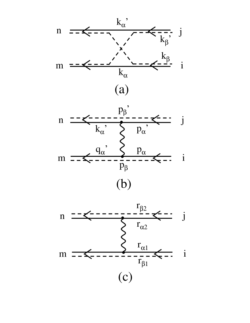
Figure 1: (a): Diagram, in the free fermion basis $(\mathbf{k}_{\alpha},\mathbf{k}_{\beta})$, for the “Pauli scattering” $\lambda\left({}^{n\ \,j}_{m\ i}\right)$ given in eq. (16), in which the “in” composite bosons $i$ and $j$ exchange their fermions $\beta$, represented by a dashed line, the “out” coboson $m$ being made with the same fermion $\alpha$ as the coboson $i$. (b): Diagram, in the free fermion basis, of the part $\xi_{1}\left({}^{n\ \,j}_{m\ i}\right)$, given in eq. (49), of the interaction scattering, due to interactions between the fermions $\alpha$ of the “in” cobosons $(i,j)$, the “out” cobosons $(m,n)$ being made with the same pairs as the “in” cobosons. (c): Same $\xi_{1}\left({}^{n\ \,j}_{m\ i}\right)$, due to $(\alpha,\alpha)$ interactions, as shown in (b), but now in real space.

The Pauli scattering $\lambda\left({}^{n\ \,j}_{m\ i}\right)$ is shown in Fig.1a. As for composite excitons, it corresponds to a fermion exchange between the “in” cobosons $(i,j)$ such that the coboson $m$ ends by having the same fermion $\alpha$ as the coboson $i$. (By convention, the cobosons of the lowest line of the Pauli scattering $\lambda\left({}^{n\ \,j}_{m\ i}\right)$, here $m$ and $i$, are made with the same fermion $\alpha$).

We can rewrite this Pauli scattering in $\mathbf{r}$ space by using

$$\langle\mathbf{k}_{\beta},\mathbf{k}_{\alpha}|i\rangle=\int d\mathbf{r}_{\alpha}\,d\mathbf{r}_{\beta}\,\langle\mathbf{k}_{\beta}|\mathbf{r}_{\beta}\rangle\,\langle\mathbf{k}_{\alpha}|\mathbf{r}_{\alpha}\rangle\,\langle\mathbf{r}_{\beta},\mathbf{r}_{\alpha}|i\rangle\ ,$$ (17)

and by performing the summation over the various $\mathbf{k}$’s through closure relations. We find that $\lambda\left({}^{n\ \,j}_{m\ i}\right)$ reads in terms of the wave functions of the $(m,n)$ and $(i,j)$ cobosons, as

$$\lambda\left({}^{n\ \,j}_{m\ i}\right)=\int d\mathbf{r}_{\alpha_{1}}\,d\mathbf{r}_{\alpha_{2}}\,d\mathbf{r}_{\beta_{1}}\,d\mathbf{r}_{\beta_{2}}\,\phi_{m}^{\ast}(\mathbf{r}_{\alpha_{1}},\mathbf{r}_{\beta_{2}})\,\phi_{n}^{\ast}(\mathbf{r}_{\alpha_{2}},\mathbf{r}_{\beta_{1}})\,\phi_{i}(\mathbf{r}_{\alpha_{1}},\mathbf{r}_{\beta_{1}})\,\phi_{j}(\mathbf{r}_{\alpha_{2}},\mathbf{r}_{\beta_{2}})\ ,$$ (18)

where $\phi_{i}(\mathbf{r}_{\alpha},\mathbf{r}_{\beta})=\langle\mathbf{r}_{\beta},\mathbf{r}_{\alpha}|i\rangle$ is the wave function of the coboson $i$ (see Fig.2a).

2.2.2 Nonorthogonal cobosons

If the cobosons form a nonorthogonal basis for one-pair states, the link between the creation operators for free fermion pairs and cobosons given in eq. (6) has to be replaced by the link given in eq. (9). From it, we now get

$$\left[D_{mi},B_{j}^{\dagger}\right]=\sum_{n}B_{n}^{\dagger}\sum_{p}\,z_{np}\,\left[\lambda\left({}^{p\ \,j}_{m\ i}\right)+\lambda\left({}^{m\ j}_{p\ \,i}\right)\right]\ ,$$ (19)

where $\lambda\left({}^{p\ \,j}_{m\ i}\right)$ is the same Pauli scattering as the one defined in eq. (16) or (18).

2.3 Scalar product of coboson states

Equation (19) for cobosons forming a nonorthogonal basis is definitely not as simple as eq. (13). This, however, has no major consequence on the scalar product of $N$-coboson states. Indeed, if we consider the scalar product of two coboson states, we find, using eq. (10),

$$\langle v|B_{m}B_{n}B_{i}^{\dagger}B_{j}^{\dagger}|v\rangle=\langle n|i\rangle\,\langle m|j\rangle+\langle n|j\rangle\,\langle m|i\rangle-\langle v|B_{m}D_{ni}B_{j}^{\dagger}|v\rangle\ ,$$ (20)

the last term of the above equation reading, due to eq. (19),

$$\langle v|B_{m}D_{ni}B_{j}^{\dagger}|v\rangle=\sum_{p,q}\langle m|p\rangle\,z_{pq}\,\left[\lambda\left({}^{q\ j}_{n\ i}\right)+\lambda\left({}^{n\ j}_{q\ i}\right)\right]\ .$$ (21)

So that, due to eq. (8), the scalar product of two-coboson states reduces to

$$\langle v|B_{m}B_{n}B_{i}^{\dagger}B_{j}^{\dagger}|v\rangle=\langle n|i\rangle\,\langle m|j\rangle+\langle n|j\rangle\,\langle m|i\rangle-\lambda\left({}^{n\ \,j}_{m\ i}\right)-\lambda\left({}^{m\ j}_{n\ \,i}\right)\ .$$ (22)

The exchange part of this scalar product is just the one for orthogonal cobosons — or for excitons [1] —, the only difference coming from the naïve part, i. e., the part which remains when cobosons are replaced by elementary particles, the scalar product $\langle m|i\rangle$ being just replaced by $\delta_{m,i}$ if the cobosons are orthogonal.

It is possible to show that this nicely simple result can be extended to more complicated scalar products of coboson states.

3 Coboson scatterings due to interactions between fermions

The cobosons interact through fermion exchanges as described in the preceding section. They also interact, in a more standard way, through the forces which exist between the fermions from which they are constructed. It is of importance to note that this second coboson interaction, which can appear as rather naïve, is in fact very subtle due to the fermion undistinguishability. Indeed, with fermions $(\alpha_{1},\alpha_{2},\beta_{1},\beta_{2})$, two kinds of cobosons can be made, $(\alpha_{1},\beta_{1})$ and $(\alpha_{2},\beta_{2})$, or $(\alpha_{1},\beta_{2})$ and $(\alpha_{2},\beta_{1})$. Due to this, the interactions between cobosons resulting from forces between fermions $\alpha$ and $\beta$, must be taken as $v(\alpha_{1},\beta_{2})+v(\alpha_{2},\beta_{1})$ in the first case, but $v(\alpha_{1},\beta_{1})+v(\alpha_{2},\beta_{2})$ in the second case. Since there is no way to know with which pairs of fermions the cobosons are made, there is no way to unambiguously write the interactions between cobosons associated to the forces between fermions $\alpha$ and $\beta$.

It is however clear that, even if the interactions between cobosons due to forces between fermions $\alpha$ and $\beta$ cannot be properly defined, these forces must play a role in the many-body physics of these cobosons. The clean way to make them appearing is actually non standard. It again relies on a set of commutators.

3.1 System Hamiltonian for fermions $\alpha$ and $\beta$

The general form for a system Hamiltonian made of fermions $\alpha$ and $\beta$ reads in first quantization as

$$H=H_{\alpha}+H_{\beta}+V_{\alpha\alpha}+V_{\beta\beta}+V_{\alpha\beta}\ .$$ (23)

$H_{\alpha}$ and $H_{\beta}$ are one-body operators for fermions $\alpha$ and fermions $\beta$:

$$H_{\alpha}=\sum_{n}h_{\alpha}(\mathbf{r}_{\alpha n})\hskip 56.9055ptH_{\beta}=\sum_{n}h_{\beta}(\mathbf{r}_{\beta n})\ .$$ (24)

The three other terms of the Hamiltonian (23) are two-body operators which correspond to interactions between cobosons $\alpha$, between cobosons $\beta$ and between cobosons $\alpha$ and $\beta$:

$$V_{\alpha\alpha}=\frac{1}{2}\sum_{n\neq n^{\prime}}v_{\alpha\alpha}(\mathbf{r}_{\alpha n},\mathbf{r}_{\alpha n^{\prime}})\ ,$$ (25)

$$V_{\alpha\beta}=\sum_{n,n^{\prime}}v_{\alpha\beta}(\mathbf{r}_{\alpha n},\mathbf{r}_{\beta n^{\prime}})\ .$$ (26)

In terms of the creation operators for the free fermion states introduced in section 2 (which, in general, are not the exact eigenstates of $h_{\alpha}$ and $h_{\beta}$), the non-interacting part of the system Hamiltonian reads

$$H_{\alpha}=\sum_{\mathbf{k}_{\alpha},\mathbf{k}_{\alpha}^{\prime}}\langle\mathbf{k}_{\alpha}^{\prime}|h_{\alpha}|\mathbf{k}_{\alpha}\rangle\,a_{\mathbf{k}_{\alpha}^{\prime}}^{\dagger}a_{\mathbf{k}_{\alpha}}\ ,$$ (27)

$$H_{\beta}=\sum_{\mathbf{k}_{\beta},\mathbf{k}_{\beta}^{\prime}}\langle\mathbf{k}_{\beta}^{\prime}|h_{\beta}|\mathbf{k}_{\beta}\rangle\,b_{\mathbf{k}_{\beta}^{\prime}}^{\dagger}b_{\mathbf{k}_{\beta}}\ ,$$ (28)

where the prefactors are given by

$$\langle\mathbf{k}_{\alpha}^{\prime}|h_{\alpha}|\mathbf{k}_{\alpha}\rangle=\int d\mathbf{r}\,\langle\mathbf{k}_{\alpha}^{\prime}|\mathbf{r}\rangle\,h_{\alpha}(\mathbf{r})\,\langle\mathbf{r}|\mathbf{k}_{\alpha}\rangle\ .$$ (29)

and similarly for $\langle\mathbf{k}_{\beta}^{\prime}|h_{\beta}|\mathbf{k}_{\beta}\rangle$. In the same way, the two-body interacting parts of the Hamiltonian $H$ read in second quantization, on this basis, as

$$V_{\alpha\alpha}=\frac{1}{2}\sum_{\mathbf{k}_{\alpha}^{\prime},\mathbf{k}_{\alpha},\mathbf{q}_{\alpha}^{\prime},\mathbf{q}_{\alpha}}v_{\alpha\alpha}\left({}^{\mathbf{q}_{\alpha}^{\prime}\ \mathbf{q}_{\alpha}}_{\mathbf{k}_{\alpha}^{\prime}\ \mathbf{k}_{\alpha}}\right)\,a_{\mathbf{k}_{\alpha}^{\prime}}^{\dagger}a_{\mathbf{q}_{\alpha}^{\prime}}^{\dagger}a_{\mathbf{q}_{\alpha}}a_{\mathbf{k}_{\alpha}}\ ,$$ (30)

$$V_{\alpha\beta}=\sum_{\mathbf{k}_{\alpha}^{\prime},\mathbf{k}_{\alpha},\mathbf{k}_{\beta}^{\prime},\mathbf{k}_{\beta}}v_{\alpha\beta}\left({}^{\mathbf{k}_{\beta}^{\prime}\ \mathbf{k}_{\beta}}_{\mathbf{k}_{\alpha}^{\prime}\ \mathbf{k}_{\alpha}}\right)\,a_{\mathbf{k}_{\alpha}^{\prime}}^{\dagger}b_{\mathbf{k}_{\beta}^{\prime}}^{\dagger}b_{\mathbf{k}_{\beta}}a_{\mathbf{k}_{\alpha}}\ ,$$ (31)

where the prefactors are given by

$$v_{\alpha\alpha}\left({}^{\mathbf{q}_{\alpha}^{\prime}\ \mathbf{q}_{\alpha}}_{\mathbf{k}_{\alpha}^{\prime}\ \mathbf{k}_{\alpha}}\right) = \int d\mathbf{r}_{\alpha}\,d\mathbf{r}_{\alpha}^{\prime}\,\langle\mathbf{k}_{\alpha}^{\prime}|\mathbf{r}_{\alpha}\rangle\,\langle\mathbf{q}_{\alpha}^{\prime}|\mathbf{r}_{\alpha}^{\prime}\rangle\,v_{\alpha\alpha}(\mathbf{r}_{\alpha},\mathbf{r}_{\alpha}^{\prime})\,\langle\mathbf{r}_{\alpha}^{\prime}|\mathbf{q}_{\alpha}\rangle\,\langle\mathbf{r}_{\alpha}|\mathbf{k}_{\alpha}\rangle$$ (32)

$$= v_{\alpha\alpha}\left({}_{\mathbf{q}_{\alpha}^{\prime}\ \mathbf{q}_{\alpha}}^{\mathbf{k}_{\alpha}^{\prime}\ \mathbf{k}_{\alpha}}\right)\ ,$$

and similarly for the other prefactors.

3.2 Orthogonal cobosons

3.2.1 “Creation potential”

Let us first consider cobosons forming an orthogonal set, these cobosons being not necessarily the exact one-pair eigenstates of the system Hamiltonian. Due to the closure relation (5) for orthogonal states, $H$ acting on $|i\rangle$ then reads

$$H|i\rangle=\sum_{m}|m\rangle\,\langle m|H|i\rangle\ ,$$ (33)

with $\langle m|H|i\rangle=E_{i}\,\delta_{m,i}$ if the cobosons are eigenstates of the system Hamiltonian, i. e., if $(H-E_{i})|i\rangle=0$. Equation (33) leads to define the “creation potential” $V_{i}^{\dagger}$ for the coboson $i$ as

$$[H,B_{i}^{\dagger}]=\sum_{m}\langle m|H|i\rangle\,B_{m}^{\dagger}+V_{i}^{\dagger}\ ,$$ (34)

in order for the creation potential to be such that

$$V_{i}^{\dagger}|v\rangle=0\ .$$ (35)

This insures $V_{i}^{\dagger}$ to indeed describe the interactions of the coboson $i$ with the rest of the system. Let us now calculate this $V_{i}^{\dagger}$ explicitly.

(i) It is possible to split the commutator of $B_{i}^{\dagger}$, given in eq. (4), with the part of the Hamiltonian acting on fermion pairs, into three terms:

$$\left[H_{\alpha}+H_{\beta}+V_{\alpha\beta},B_{i}^{\dagger}\right]=A_{1}^{\dagger}+A_{2}^{\dagger}+A_{3}^{\dagger}\ ,$$ (36)

with $A_{1}^{\dagger}$ in $a^{\dagger}b^{\dagger}$, $A_{2}^{\dagger}$ in $a^{\dagger}b^{\dagger}b^{\dagger}b$ and $A_{3}^{\dagger}$ in $a^{\dagger}b^{\dagger}a^{\dagger}a$. The first term $A_{1}^{\dagger}$ precisely reads

$$A_{1}^{\dagger}=\sum_{\mathbf{k}_{\alpha}^{\prime},\mathbf{p}_{\beta}}a_{\mathbf{k}_{\alpha}^{\prime}}^{\dagger}b_{\mathbf{p}_{\beta}}^{\dagger}\,\sum_{\mathbf{p}_{\alpha}}\langle\mathbf{k}_{\alpha}^{\prime}|h_{\alpha}|\mathbf{p}_{\alpha}\rangle\,\langle\mathbf{p}_{\beta},\mathbf{p}_{\alpha}|i\rangle+\sum_{\mathbf{k}_{\beta}^{\prime},\mathbf{p}_{\alpha}}a_{\mathbf{p}_{\alpha}}^{\dagger}b_{\mathbf{k}_{\beta}^{\prime}}^{\dagger}\,\sum_{\mathbf{p}_{\beta}}\langle\mathbf{k}_{\beta}^{\prime}|h_{\beta}|\mathbf{p}_{\beta}\rangle\,\langle\mathbf{p}_{\beta},\mathbf{p}_{\alpha}|i\rangle$$

$$+\sum_{\mathbf{k}_{\alpha}^{\prime},\mathbf{k}_{\beta}^{\prime}}a_{\mathbf{k}_{\alpha}^{\prime}}^{\dagger}b_{\mathbf{k}_{\beta}^{\prime}}^{\dagger}\,\sum_{\mathbf{p}_{\alpha},\mathbf{p}_{\beta}}v_{\alpha\beta}\left({}^{\mathbf{k}_{\beta}^{\prime}\ \mathbf{p}_{\beta}}_{\mathbf{k}_{\alpha}^{\prime}\ \mathbf{p}_{\alpha}}\right)\,\langle\mathbf{p}_{\beta},\mathbf{p}_{\alpha}|i\rangle\ .$$ (37)

By noting that $H_{\alpha}$ does not act on fermion $\beta$, while the prefactor of the last term is nothing but

$$v_{\alpha\beta}\left({}^{\mathbf{k}_{\beta}^{\prime}\ \mathbf{p}_{\beta}}_{\mathbf{k}_{\alpha}^{\prime}\ \mathbf{p}_{\alpha}}\right)=\langle\mathbf{k}_{\beta}^{\prime},\mathbf{k}_{\alpha}^{\prime}|V_{\alpha\beta}|\mathbf{p}_{\alpha},\mathbf{p}_{\beta}\rangle\ ,$$

it is easy to see that $A_{1}^{\dagger}$ can be rewritten in a compact form as

$$A_{1}^{\dagger}=\sum_{\mathbf{k}_{\alpha}^{\prime},\mathbf{k}_{\beta}^{\prime}}a_{\mathbf{k}_{\alpha}^{\prime}}^{\dagger}b_{\mathbf{k}_{\beta}^{\prime}}^{\dagger}\,\sum_{\mathbf{p}_{\alpha},\mathbf{p}_{\beta}}\langle\mathbf{k}_{\beta}^{\prime},\mathbf{k}_{\alpha}^{\prime}|H_{\alpha}+H_{\beta}+V_{\alpha\beta}|\mathbf{p}_{\alpha},\mathbf{p}_{\beta}\rangle\,\langle\mathbf{p}_{\beta},\mathbf{p}_{\alpha}|i\rangle\ .$$ (38)

If we now use eq. (6) to write $a^{\dagger}b^{\dagger}$ in terms of cobosons, we end, due to eq. (2), with

$$A_{1}^{\dagger}=\sum_{m}\langle m|H|i\rangle\,B_{m}^{\dagger}\ ,$$ (39)

which is just the first term of eq. (34).

The second term on the RHS of eq. (36), $A_{2}^{\dagger}$, appears as

$$A_{2}^{\dagger}=\sum_{\mathbf{k}_{\alpha}^{\prime},\mathbf{p}_{\beta}}a_{\mathbf{k}_{\alpha}^{\prime}}^{\dagger}b_{\mathbf{p}_{\beta}}^{\dagger}\,\sum_{\mathbf{k}_{\beta}^{\prime},\mathbf{k}_{\beta}}b_{\mathbf{k}_{\beta}^{\prime}}^{\dagger}b_{\mathbf{k}_{\beta}}\,\sum_{\mathbf{p}_{\alpha}}v_{\alpha\beta}\left({}^{\mathbf{k}_{\beta}^{\prime}\ \mathbf{k}_{\beta}}_{\mathbf{k}_{\alpha}^{\prime}\ \mathbf{p}_{\alpha}}\right)\,\langle\mathbf{p}_{\beta},\mathbf{p}_{\alpha}|i\rangle\ .$$ (40)

We rewrite the first $a^{\dagger}b^{\dagger}$ in terms of coboson operators according to eq. (6), to make $A_{2}^{\dagger}$ reading as

$$A_{2}^{\dagger}=\sum_{m}B_{m}^{\dagger}\,\sum_{\mathbf{k}_{\beta}^{\prime},\mathbf{k}_{\beta}}b_{\mathbf{k}_{\beta}^{\prime}}^{\dagger}b_{\mathbf{k}_{\beta}}\,X_{\alpha\beta}(\mathbf{k}_{\beta}^{\prime},\mathbf{k}_{\beta};m,i)\ ,$$

$$X_{\alpha\beta}(\mathbf{k}_{\beta}^{\prime},\mathbf{k}_{\beta};m,i)=\sum_{\mathbf{k}_{\alpha}^{\prime},\mathbf{p}_{\alpha},\mathbf{p}_{\beta}}\langle m|\mathbf{k}_{\alpha}^{\prime},\mathbf{p}_{\beta}\rangle\,v_{\alpha\beta}\left({}^{\mathbf{k}_{\beta}^{\prime}\ \mathbf{k}_{\beta}}_{\mathbf{k}_{\alpha}^{\prime}\ \mathbf{p}_{\alpha}}\right)\,\langle\mathbf{p}_{\beta},\mathbf{p}_{\alpha}|i\rangle\ .$$ (41)

In the same way, $A_{3}^{\dagger}$ is found to be

$$A_{3}^{\dagger}=\sum_{m}B_{m}^{\dagger}\,\sum_{\mathbf{k}_{\alpha}^{\prime},\mathbf{k}_{\alpha}}a_{\mathbf{k}_{\alpha}^{\prime}}^{\dagger}a_{\mathbf{k}_{\alpha}}\,Y_{\alpha\beta}(\mathbf{k}_{\alpha}^{\prime},\mathbf{k}_{\alpha};m,i)\ ,$$

$$Y_{\alpha\beta}(\mathbf{k}_{\alpha}^{\prime},\mathbf{k}_{\alpha};m,i)=\sum_{\mathbf{k}_{\beta}^{\prime},\mathbf{p}_{\alpha},\mathbf{p}_{\beta}}\langle m|\mathbf{p}_{\alpha},\mathbf{k}_{\beta}^{\prime}\rangle\,v_{\alpha\beta}\left({}^{\mathbf{k}_{\beta}^{\prime}\ \mathbf{p}_{\beta}}_{\mathbf{k}_{\alpha}^{\prime}\ \mathbf{k}_{\alpha}}\right)\,\langle\mathbf{p}_{\beta},\mathbf{p}_{\alpha}|i\rangle\ .$$ (42)

(ii) If we now turn to the interactions between fermions $\alpha$, the same procedure leads to

$$\left[V_{\alpha\alpha},B_{i}^{\dagger}\right]=\sum_{m}B_{m}^{\dagger}\,\sum_{\mathbf{k}_{\alpha}^{\prime},\mathbf{k}_{\alpha}}a_{\mathbf{k}_{\alpha}^{\prime}}^{\dagger}a_{\mathbf{k}_{\alpha}}\,Y_{\alpha\alpha}(\mathbf{k}_{\alpha}^{\prime},\mathbf{k}_{\alpha};m,i)\ ,$$

$$Y_{\alpha\alpha}(\mathbf{k}_{\alpha}^{\prime},\mathbf{k}_{\alpha};m,i)=\sum_{\mathbf{q}_{\alpha}^{\prime},\mathbf{p}_{\alpha},\mathbf{p}_{\beta}}\langle m|\mathbf{q}_{\alpha}^{\prime},\mathbf{p}_{\beta}\rangle\,v_{\alpha\alpha}\left({}_{\mathbf{q}_{\alpha}^{\prime}\ \mathbf{p}_{\alpha}}^{\mathbf{k}_{\alpha}^{\prime}\ \mathbf{k}_{\alpha}}\right)\,\langle\mathbf{p}_{\beta},\mathbf{p}_{\alpha}|i\rangle\ ,$$ (43)

while the interactions between fermions $\beta$ give

$$\left[V_{\beta\beta},B_{i}^{\dagger}\right]=\sum_{m}B_{m}^{\dagger}\,\sum_{\mathbf{k}_{\beta}^{\prime},\mathbf{k}_{\beta}}b_{\mathbf{k}_{\beta}^{\prime}}^{\dagger}b_{\mathbf{k}_{\beta}}\,X_{\beta\beta}(\mathbf{k}_{\beta}^{\prime},\mathbf{k}_{\beta};m,i)\ ,$$

$$X_{\beta\beta}(\mathbf{k}_{\beta}^{\prime},\mathbf{k}_{\beta};m,i)=\sum_{\mathbf{q}_{\beta}^{\prime},\mathbf{p}_{\alpha},\mathbf{p}_{\beta}}\langle m|\mathbf{p}_{\alpha},\mathbf{q}_{\beta}^{\prime}\rangle\,v_{\beta\beta}\left({}_{\mathbf{q}_{\beta}^{\prime}\ \mathbf{p}_{\beta}}^{\mathbf{k}_{\beta}^{\prime}\ \mathbf{k}_{\beta}}\right)\,\langle\mathbf{p}_{\beta},\mathbf{p}_{\alpha}|i\rangle\ ,$$ (44)

(iii) By collecting the results of eqs. (36,39,41,42-44), the creation potential $V_{i}^{\dagger}$, defined in eq. (34), finally reads

$$V_{i}^{\dagger}=\sum_{m}B_{m}^{\dagger}\,W_{mi}\ ,$$

where the operator $W_{mi}$ is defined by

$$W_{mi} = \sum_{\mathbf{k}_{\alpha}^{\prime},\mathbf{k}_{\alpha}}a_{\mathbf{k}_{\alpha}^{\prime}}^{\dagger}a_{\mathbf{k}_{\alpha}}\left[Y_{\alpha\alpha}(\mathbf{k}_{\alpha}^{\prime},\mathbf{k}_{\alpha};m,i)+Y_{\alpha\beta}(\mathbf{k}_{\alpha}^{\prime},\mathbf{k}_{\alpha};m,i)\right]$$ (45)

$$+ \sum_{\mathbf{k}_{\beta}^{\prime},\mathbf{k}_{\beta}}b_{\mathbf{k}_{\beta}^{\prime}}^{\dagger}b_{\mathbf{k}_{\beta}}\left[X_{\beta\beta}(\mathbf{k}_{\beta}^{\prime},\mathbf{k}_{\beta};m,i)+X_{\alpha\beta}(\mathbf{k}_{\beta}^{\prime},\mathbf{k}_{\beta};m,i)\right]\ .$$

Since $W_{mi}|v\rangle=0$, it is thus easy to check that the condition (35) for a creation potential, is indeed fulfilled by this $V_{i}^{\dagger}$.

3.2.2 “Interaction scatterings”

The “direct interaction scatterings” between cobosons $i$ and $j$ physically come from the interactions between fermions $(\alpha,\alpha)$, between fermions $(\beta,\beta)$ and also from the interactions between fermions $(\alpha,\beta)$, with the part between the fermions $(\alpha,\beta)$ making the coboson $i$ excluded. These interaction scatterings are formally defined through

$$\left[V_{i}^{\dagger},B_{j}^{\dagger}\right]=\sum_{mn}\xi\left({}^{n\ \,j}_{m\ i}\right)\,B_{m}^{\dagger}B_{n}^{\dagger}\ ,$$ (46)

so that these scatterings are such that

$$\left[W_{mi},B_{j}^{\dagger}\right]=\sum_{n}\xi\left({}^{n\ \,j}_{m\ i}\right)\,B_{n}^{\dagger}\ .$$ (47)

To calculate $\xi$, let us consider the first term of eq. (45), in $Y_{\alpha\alpha}$. Using eqs. (4,6), the commutator of this first term with $B_{j}^{\dagger}$ reads

$$[W_{mi}^{(1)},B_{j}^{\dagger}] = \sum_{\mathbf{k}_{\alpha}^{\prime},\mathbf{k}_{\alpha}}\sum_{\mathbf{p}_{\alpha}^{\prime},\mathbf{p}_{\beta}^{\prime}}Y_{\alpha\alpha}(\mathbf{k}_{\alpha}^{\prime},\mathbf{k}_{\alpha};m,i)\,\langle\mathbf{p}_{\beta}^{\prime},\mathbf{p}_{\alpha}^{\prime}|j\rangle\,[a_{\mathbf{k}_{\alpha}^{\prime}}^{\dagger}a_{\mathbf{k}_{\alpha}},a_{\mathbf{p}_{\alpha}^{\prime}}^{\dagger}b_{\mathbf{p}_{\beta}^{\prime}}^{\dagger}]$$ (48)

$$= \sum_{\mathbf{k}_{\alpha}^{\prime},\mathbf{p}_{\alpha}^{\prime},\mathbf{p}_{\beta}^{\prime}}Y_{\alpha\alpha}(\mathbf{k}_{\alpha}^{\prime},\mathbf{p}_{\alpha}^{\prime};m,i)\,\langle\mathbf{p}_{\beta}^{\prime},\mathbf{p}_{\alpha}^{\prime}|j\rangle\,\sum_{n}B_{n}^{\dagger}\,\langle n|\mathbf{k}_{\alpha}^{\prime},\mathbf{p}_{\beta}^{\prime}\rangle\ .$$

By inserting $Y_{\alpha\alpha}$ given in eq. (43) into the above equation, we find that the first term of $\xi\left({}^{n\ \,j}_{m\ i}\right)$ reads

$$\xi_{1}\left({}^{n\ \,j}_{m\ i}\right)=\sum_{\mathbf{k}_{\alpha}^{\prime},\mathbf{q}_{\alpha}^{\prime},\mathbf{p}_{\alpha}^{\prime},\mathbf{p}_{\beta}^{\prime},\mathbf{p}_{\alpha},\mathbf{p}_{\beta}}\langle m|\mathbf{q}_{\alpha}^{\prime},\mathbf{p}_{\beta}\rangle\,\langle n|\mathbf{k}_{\alpha}^{\prime},\mathbf{p}_{\beta}^{\prime}\rangle\,v_{\alpha\alpha}\left({}_{\mathbf{q}_{\alpha}^{\prime}\ \mathbf{p}_{\alpha}}^{\mathbf{k}_{\alpha}^{\prime}\ \mathbf{p}_{\alpha}^{\prime}}\right)\,\langle\mathbf{p}_{\beta},\mathbf{p}_{\alpha}|i\rangle\,\langle\mathbf{p}_{\beta}^{\prime},\mathbf{p}_{\alpha}^{\prime}|j\rangle\ .$$ (49)

This $\xi_{1}\left({}^{n\ \,j}_{m\ i}\right)$ is shown in Fig.1b. It corresponds to an interaction between the fermions $\alpha$ of the “in” cobosons $(i,j)$, the “out” cobosons $(m,n)$ being made with the same fermion pair as the “in” cobosons. We can rewrite this $\xi_{1}$ in real space, by using eqs. (17) and (32) and by performing the summation over the various $\mathbf{k}$’s through closure relations. This leads to

$$\xi_{1}\left({}^{n\ \,j}_{m\ i}\right)=\int d\mathbf{r}_{\alpha 1}d\mathbf{r}_{\alpha 2}d\mathbf{r}_{\beta 1}d\mathbf{r}_{\beta 2}\phi_{m}^{\ast}(\mathbf{r}_{\alpha 1},\mathbf{r}_{\beta 1})\phi_{n}^{\ast}(\mathbf{r}_{\alpha 2},\mathbf{r}_{\beta 2})v_{\alpha\alpha}(\mathbf{r}_{\alpha 1},\mathbf{r}_{\alpha 2})\phi_{i}(\mathbf{r}_{\alpha 1},\mathbf{r}_{\beta 1})\phi_{j}(\mathbf{r}_{\alpha 2},\mathbf{r}_{\beta 2})\ ,$$ (50)

which is shown in Fig.1c.

By calculating the contributions of the three other terms of eq. (45) in the same way, we end with a direct interaction scattering which has a form very similar to the one for excitons [1], namely

$$\xi\left({}^{n\ \,j}_{m\ i}\right)=\int d\mathbf{r}_{\alpha 1}\,d\mathbf{r}_{\alpha 2}\,d\mathbf{r}_{\beta 1}\,d\mathbf{r}_{\beta 2}\,\phi_{m}^{\ast}(\mathbf{r}_{\alpha 1},\mathbf{r}_{\beta 1})\,\phi_{n}^{\ast}(\mathbf{r}_{\alpha 2},\mathbf{r}_{\beta 2})\,\phi_{i}(\mathbf{r}_{\alpha 1},\mathbf{r}_{\beta 1})\,\phi_{j}(\mathbf{r}_{\alpha 2},\mathbf{r}_{\beta 2})$$

$$\times\ \left[v_{\alpha\alpha}(\mathbf{r}_{\alpha 1},\mathbf{r}_{\alpha 2})+v_{\beta\beta}(\mathbf{r}_{\beta 1},\mathbf{r}_{\beta 2})+v_{\alpha\beta}(\mathbf{r}_{\alpha 1},\mathbf{r}_{\beta 2})+v_{\alpha\beta}(\mathbf{r}_{\alpha 2},\mathbf{r}_{\beta 1})\right]\ .$$ (51)

This direct scattering is represented in Fig.2b: In it, no fermion exchange takes place between the “in” cobosons $(i,j)$.

3.2.3 Matrix elements of the system Hamiltonian in the 2-coboson subspace

Using the commutators given in eqs. (34,46), the Hamiltonian in the two-coboson subspace appears as

$$\langle v|B_{m}B_{n}\,H\,B_{i}^{\dagger}B_{j}^{\dagger}|v\rangle=\sum_{q}\langle v|B_{m}B_{n}B_{i}^{\dagger}B_{q}^{\dagger}|v\rangle\,\langle q|H|j\rangle\ +\ (i\leftrightarrow j)$$

$$+\sum_{pq}\xi\left({}^{q\ j}_{p\ i}\right)\,\langle v|B_{m}B_{n}B_{p}^{\dagger}B_{q}^{\dagger}|v\rangle\ .$$ (52)

So that, using eq. (22 ) for the scalar product of orthogonal cobosons, we end with

$$\langle v|B_{m}B_{n}\,H\,B_{i}^{\dagger}B_{j}^{\dagger}|v\rangle=\left[\delta_{m,i}\,\langle n|H|j\rangle+\delta_{n,i}\,\langle m|H|j\rangle-\sum_{q}\left(\lambda\left({}^{n\ \,q}_{m\ i}\right)+\lambda\left({}^{m\ q}_{n\ \,i}\right)\right)\langle q|H|j\rangle\right.$$

$$\left.+\xi\left({}^{n\ \,j}_{m\ i}\right)-\xi^{\mathrm{in}}\left({}^{n\ \,j}_{m\ i}\right)\right]\ +[i\leftrightarrow j]\ ,$$ (53)

where $\xi^{\mathrm{in}}$ is the exchange interaction scattering shown in Fig.2c. It is precisely given by

$$\xi^{\mathrm{in}}\left({}^{n\ \,j}_{m\ i}\right) = \sum_{pq}\lambda\left({}^{n\ \,q}_{m\ p}\right)\,\xi\left({}^{q\ j}_{p\ i}\right)$$ (54)

$$= \int d\mathbf{r}_{\alpha 1}\,d\mathbf{r}_{\beta 1}\,d\mathbf{r}_{\alpha 2}\,d\mathbf{r}_{\beta 2}\,\langle m|\mathbf{r}_{\alpha 1},\mathbf{r}_{\beta 2}\rangle\,\langle n|\mathbf{r}_{\alpha 2},\mathbf{r}_{\beta 1}\rangle\,\langle\mathbf{r}_{\beta 1},\mathbf{r}_{\alpha 1}|i\rangle\,\langle\mathbf{r}_{\beta 2},\mathbf{r}_{\alpha 2}|j\rangle$$

$$\times \ \left[v_{\alpha\alpha}(\mathbf{r}_{\alpha 1},\mathbf{r}_{\alpha 2})+v_{\beta\beta}(\mathbf{r}_{\beta 1},\mathbf{r}_{\beta 2})+v_{\alpha\beta}(\mathbf{r}_{\alpha 1},\mathbf{r}_{\beta 2})+v_{\alpha\beta}(\mathbf{r}_{\alpha 2},\mathbf{r}_{\beta 1})\right]\ .$$

In the case of coboson eigenstates of the system Hamiltonian, $\langle n|H|j\rangle=E_{j}\,\delta_{n,j}$, we readily recover the result for composite excitons [1].

3.3 Nonorthogonal cobosons

If the coboson states form a complete set for one-fermion-pair states, but if these states are not orthogonal, we expect the preceding results to be far more complicated. It turns out that, as for the scalar product of cobosons, given in eq. (22), the only difference with the results for orthogonal cobosons comes from the naïve part.

3.3.1 Creation potential and interaction scattering

Let us briefly go through the same path as the one we used in the preceding subsection, the closure relation for cobosons being now given by eq. (7).

The definition of the creation potential for the coboson $i$, given in eq. (34) for orthogonal cobosons, now reads

$$\left[H,B_{i}^{\dagger}\right]=\sum_{m}B_{m}^{\dagger}\,\sum_{q}z_{mq}\,\langle q|H|i\rangle+V_{i}^{\dagger}\ ,$$ (55)

in order to still have $V_{i}^{\dagger}|v\rangle=0$. From the precise calculation of $V_{i}^{\dagger}$, we can then show, by using eq. (9) to write $a^{\dagger}b^{\dagger}$ in terms of cobosons, that

$$V_{i}^{\dagger}=\sum_{mq}B_{m}^{\dagger}\,z_{mq}\,W_{qi}\ ,$$ (56)

$$\left[V_{i}^{\dagger},B_{j}^{\dagger}\right]=\sum_{mn}B_{m}^{\dagger}B_{n}^{\dagger}\sum_{pq}z_{mp}\,z_{nq}\,\xi\left({}^{q\ j}_{p\ i}\right)\ ,$$ (57)

where $W_{qi}$ is defined in eq. (45) and $\xi$ is the direct interaction scattering defined in eq. (51).

3.3.2 Matrix elements of the system Hamiltonian in the 2-coboson subspace

Using eqs. (55,57), we readily find

$$\langle v|B_{m}B_{n}HB_{i}^{\dagger}B_{j}^{\dagger}|v\rangle=\langle v|B_{m}B_{n}B_{i}^{\dagger}HB_{j}^{\dagger}|v\rangle\ +(i\leftrightarrow j)\ +\sum_{pqtu}\langle v|B_{m}B_{n}B_{p}^{\dagger}B_{q}^{\dagger}|v\rangle\,z_{pt}z_{qu}\,\xi\left({}^{u\ j}_{t\ i}\right)\ .$$ (58)

The closure relation (7) allows to write the first term of the above equation as

$$\langle v|B_{m}B_{n}B_{i}^{\dagger}HB_{j}^{\dagger}|v\rangle=\sum_{pq}\langle v|B_{m}B_{n}B_{i}^{\dagger}B_{p}^{\dagger}|v\rangle\,z_{pq}\,\langle q|H|j\rangle\ ,$$ (59)

so that, using the scalar product of coboson states given in eq. (22), this first term reads

$$\langle v|B_{m}B_{n}B_{i}^{\dagger}HB_{j}^{\dagger}|v\rangle=\langle n|i\rangle\,\langle m|H|j\rangle+\langle m|i\rangle\,\langle n|H|j\rangle-\sum_{pq}\left[\lambda\left({}^{n\ \,p}_{m\ i}\right)+\lambda\left({}^{m\ p}_{n\ \,i}\right)\right]z_{pq}\,\langle q|H|j\rangle\ ,$$ (60)

If we now turn to the last term of eq. (58), we find, from the same eq. (22),

$$\sum_{pqtu}\langle v|B_{m}B_{n}B_{p}^{\dagger}B_{q}^{\dagger}|v\rangle\,z_{pt}z_{qu}\,\xi\left({}^{u\ j}_{t\ i}\right)=\sum_{pqtu}\langle m|p\rangle\,\langle n|q\rangle\,z_{pt}\,z_{qu}\,\xi\left({}^{u\ j}_{t\ i}\right)\hskip 85.35826pt$$

$$-\sum_{pqtu}\lambda\left({}^{n\ \,q}_{m\ p}\right)\,z_{pt}\,z_{qu}\,\xi\left({}^{u\ j}_{t\ i}\right)\ +\ (m\leftrightarrow n)\ .$$ (61)

The first term readily gives $\xi\left({}^{n\ \,j}_{m\ i}\right)$, due to eq. (8). By using the expressions of $\lambda$ and $\xi$ in $\mathbf{r}$ space given in eqs. (18,51), the second term appears as

$$\sum_{pqtu}\lambda\left({}^{n\ \,q}_{m\ p}\right)\,z_{pt}\,z_{qu}\,\xi\left({}^{u\ j}_{t\ i}\right)=\sum_{pqtu}z_{pt}\,z_{qu}\int\{d\mathbf{r}\}\,d\{\mathbf{r}^{\prime}\}\,\langle m|\mathbf{r}_{\alpha 1}^{\prime},\mathbf{r}_{\beta_{2}}^{\prime}\rangle\,\langle n|\mathbf{r}_{\alpha 2}^{\prime},\mathbf{r}_{\beta 1}^{\prime}\rangle\,\langle\mathbf{r}_{\beta 1}^{\prime}\mathbf{r}_{\alpha 1}^{\prime}|p\rangle$$

$$\times\,\langle\mathbf{r}_{\beta 2}^{\prime},\mathbf{r}_{\alpha 2}^{\prime}|q\rangle\,\langle t|\mathbf{r}_{\alpha 1},\mathbf{r}_{\beta 1}\rangle\,\langle u|\mathbf{r}_{\alpha 2},\mathbf{r}_{\beta 2}\rangle\left[v_{\alpha\alpha}(\mathbf{r}_{\alpha 1},\mathbf{r}_{\alpha 2})+v_{\beta\beta}(\mathbf{r}_{\beta 1},\mathbf{r}_{\beta 2})\right.$$

$$\left.+v_{\alpha\beta}(\mathbf{r}_{\alpha 1},\mathbf{r}_{\beta 2})+v_{\alpha\beta}(\mathbf{r}_{\alpha 2},\mathbf{r}_{\beta 1})\right]\,\langle\mathbf{r}_{\beta 1},\mathbf{r}_{\alpha 1}|i\rangle\,\langle\mathbf{r}_{\beta 2},\mathbf{r}_{\alpha 2}|j\rangle\ .\hskip 28.45274pt$$ (62)

The summations over $(p,t)$ and $(q,u)$ being performed through eq. (7), we readily find that the sum (62) reduces to the exchange interaction scattering $\xi^{\mathrm{in}}\left({}^{n\ \,j}_{m\ i}\right)$ given in eq. (54).

The above results thus show that the matrix elements of the system Hamiltonian in an arbitrary two-coboson subspace are given by

$$\langle v|B_{m}B_{n}HB_{i}^{\dagger}B_{j}^{\dagger}|v\rangle=\left\{\left[\langle n|i\rangle\,\langle m|H|j\rangle-\sum_{pq}\lambda\left({}^{n\ \,p}_{m\ i}\right)\,z_{pq}\,\langle q|H|j\rangle\right]+[i\leftrightarrow j]\right.$$

$$\left.+\xi\left({}^{n\ \,j}_{m\ i}\right)-\xi^{\mathrm{in}}\left({}^{n\ \,j}_{m\ i}\right)\right\}+\{m\leftrightarrow n\}\ .$$ (63)

This result, which reduces to eq. (53) when the coboson states are orthogonal, again show that the part coming from interactions between cobosons is formally the same whatever is the complete set of states these cobosons form.

4 Many-body effects with arbitrary cobosons

The standard way to derive many-body effects between elementary quantum particles for which the system Hamiltonian splits as $H=H_{0}+V$, goes through the iteration of

$$\frac{1}{a-H}=\frac{1}{a-H_{0}}+\frac{1}{a-H}\,V\,\frac{1}{a-H_{0}}\ .$$ (64)

We have shown [2] that, in the case of composite excitons which are eigenstates of the semiconductor Hamiltonian, the equivalent of $H=H_{0}+V$, deduced from $[H,B_{i}^{\dagger}]=E_{i}B_{i}^{\dagger}+V_{i}^{\dagger}$, is $HB_{i}^{\dagger}=(H+E_{i})B_{i}^{\dagger}+V_{i}^{\dagger}$, so that the equivalent of eq. (64) reads

$$\frac{1}{a-H}\,B_{i}^{\dagger}=B_{i}^{\dagger}\,\frac{1}{a-H-E_{i}}+\frac{1}{a-H}\,V_{i}^{\dagger}\,\frac{1}{a-H-E_{i}}\ .$$ (65)

In the most general case considered in this work, the creation potential of the coboson $i$ is defined through

$$[H,B_{i}^{\dagger}] = \sum_{m}B_{m}^{\dagger}\sum_{q}z_{mq}\,\langle q|H|i\rangle+V_{i}^{\dagger}$$ (66)

$$= H_{ii}\,B_{i}^{\dagger}+v_{i}^{\dagger}+V_{i}^{\dagger}\ ,$$

where we have set

$$H_{mi}=\sum_{q}z_{mq}\,\langle q|H|i\rangle\ \ \mathrm{and}\ \ v_{i}^{\dagger}=\sum_{m\neq i}B_{m}^{\dagger}\,H_{mi}\ .$$

$v_{i}^{\dagger}$ is such that $v_{i}^{\dagger}|v\rangle\neq 0$, while $[v_{i}^{\dagger},B_{j}^{\dagger}]=0$. The equivalent of eq. (65) then reads

$$\frac{1}{a-H}\,B_{i}^{\dagger}=B_{i}^{\dagger}\frac{1}{a-H-H_{ii}}+\frac{1}{a-H}\,(v_{i}^{\dagger}+V_{i}^{\dagger})\,\frac{1}{a-H-H_{ii}}\ .$$ (67)

Using eq. (67) which is not far more complicated than eq. (65), we can follow the same procedure as the one used for excitons, to deduce the part of the many-body effects between arbitrary cobosons coming from interactions between the elementary fermions making these composite bosons. Their correlations read in terms of matrix elements between $N$-coboson states which look like

$$\langle v|B_{m_{N}}\cdots B_{m_{1}}\,\frac{1}{a-H}\,B_{i_{1}}^{\dagger}\cdots B_{i_{N}}^{\dagger}|v\rangle\ .$$

To calculate them, we first push $1/(a-H)$ to the right according to eq. (67) and we eliminate the various “creation potentials” through eq. (46) or (57). This makes appearing a lot of interaction scatterings $\xi$. We end with scalar products of $N$-coboson states, which do not contain the system Hamiltonian anymore. These scalar products are then calculated, as for excitons, in terms of Pauli scatterings between two cobosons, using eq. (10) and eq. (13) or (19) — as done to get eq. (22) for just $N=2$ cobosons. When $N$ is large, these scalar products are better represented by Shiva diagrams for fermion exchanges between $P$ excitons, with $2\leq P\leq N$, as explained more in details in a forthcoming publication [11].

5 Conclusion

In conclusion, the present work shows how the concepts we have recently introduced to exactly treat the subtle carrier exchanges which take place in the many-body physics of excitons, can be extended to arbitrary pairs of fermions. The correct description of composite boson many-body effects relies on two sets of scatterings: the “Pauli scatterings” for fermion exchanges without interaction and the “interaction scatterings” for interaction without fermion exchange. To derive these scatterings, it is not necessary for the fermion pairs to be the exact eigenstates of the system Hamiltonian, nor to form an orthogonal set.

Figure 2: (a): Diagram for the “Pauli scattering” $\lambda\left({}^{n\ \,j}_{m\ i}\right)$, shown in Fig.1a, but now in real space. (b): Diagram, in real space, for the “interaction scattering” $\xi\left({}^{n\ \,j}_{m\ i}\right)$, defined in eq. (51), in which the “in” cobosons interact through the interactions of the fermions from which they are constructed, the “in” and “out” cobosons being made with the same fermion pairs $(\alpha_{1},\beta_{1})$ and $(\alpha_{2},\beta_{2})$. (c): Diagram, in real space, for $\xi^{\mathrm{in}}\left({}^{n\ \,j}_{m\ i}\right)$, defined in eq. (54), which is a mixed exchange-interaction scattering, the interactions taking place before the fermion exchange, i. e., between the “in” cobosons $(i,j)$.

References

[1]
M. Combescot, O. Betbeder-Matibet, Europhys. Lett. 58, 87
(2002)
[2]
For a short review, see M. Combescot, O. Betbeder-Matibet, Solid State
Comm. 134, 11 (2005)
[3]
M. Combescot, O. Betbeder-Matibet, Eur. Phys. J. B 48, 469
(2005)
[5]
H. Haug, S. Schmitt-Rink, Prog. Quantum Electron. 9, 3 (1984)
[6]
M. Combescot, O. Betbeder-Matibet, Solid State Comm. 132, 129
(2004)
[7]
M. Combescot, O. Betbeder-Matibet, K. Cho, H. Ajiki, Europhys. Lett. 72, 618 (2005)
[8]
M. Combescot, O. Betbeder-Matibet, Cond-mat/0505746, submitted to Phys. Rev. B
[9]
M. Combescot, O. Betbeder-Matibet, Phys. Rev. Lett. 93,
016403 (2004)
[10]
M. Combescot, O. Betbeder-Matibet, V. Voliotis, cond-mat/0604135, to
appear in Europhys. Lett.
[11]
M. Combescot, O. Betbeder-Matibet (preprint)