Phase Diagram for Self-assembly of Amphiphilic Molecule C₁₂E₆ by Dissipative Particle Dynamics Simulation

Abstract

In a previous study, dissipative particle dynamics simulation was used to qualitatively clarify the phase diagram of the amphiphilic molecule hexaethylene glycol dodecyl ether (C₁₂E₆). In the present study, the hydrophilicity dependence of the phase structure was clarified qualitatively by varying the interaction potential between hydrophilic molecules and water molecules in a dissipative particle dynamics (DPD) simulation using the Jury model. By varying the coefficient of the interaction potential $x$ between hydrophilic beads and water molecules as $x=-20,0,10,$ and $20,$ at a dimensionless temperature of $T=0.5$ and a concentration of amphiphilic molecules in water of $\phi=50\%,$ the phase structures grew to lamellar ($x=-20$), hexagonal ($x=0$), and micellar ($x=10$) phases. For $x=20,$ phase separation occurs between hydrophilic beads and water molecules.

1 Introduction

The phase structure of amphiphilic molecules has been extensively investigated as a typical example of soft matter physics. For the present study, we selected hexaethylene glycol dodecyl ether (C₁₂E₆), a popular surfactant in water that has various self-assembled structures.

The phase structure of C₁₂E₆ was investigated by Mitchell[1] in 1983. In recent years, phase diagrams at equilibrium, as well as non-equilibrium and steady-state conditions have been investigated (see Ref. [2]). Israelachvili proposed the packing parameter as a means of clarifying the relationship between macroscopic structure and microscopic molecular shape[3, 4]. The packing parameter $p$ is the ratio of the volume $V$ occupied by the hydrophobic tail to the product of the sectional area of a hydrophilic group $S$ and the “maximum effective length ($l$)” of the hydrophobic tail (see Fig. 1). Spherical micelles are expected when $p\leq 1/3$. When $1/3\leq p\leq 1/2,$ cylinders are expected, and for $p\sim 1,$ bilayers should form.

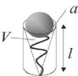
Figure 1: Schematic diagram of packing parameter[3, 4]. A gray ball and a twisting black line are used to denote the hydrophilic and hydrophobic parts, respectively, of an amphiphilic molecule. The packing parameter $p\equiv V/Sl$ controls the shape of the aggregates. Here, the parameter $V$ is the volume occupied by the hydrophobic tail, $S$ denotes the sectional area of a hydrophilic group, and $l$ is the “maximum effective length” of the hydrophobic tail.

The concept of the packing parameter is intuitive and acceptable. However, calculating the packing parameter is very difficult, even by computer simulation, because it is almost impossible to derive macroscopic phase structure at the microscopic level by simulation, using techniques such as molecular dynamics (MD) simulation, for example. In order to overcome the gap between macroscopic behavior and microscopic motion, dissipative particle dynamics (DPD) simulation has been proposed as a new mesoscopic motion simulation technique[5, 6, 7, 8]. The DPD algorithm might be considered as one of the coarse-grained methods of molecular dynamics (MD) simulation.

In 1999, using an empirical method, Jury et al. succeeded in the DPD simulation of the smectic mesophase of a simple amphiphilic molecule system with water solvent[9]. Their minimal model (herein referred to as the Jury model), which is composed of rigid AB dimers in a solvent composed of W monomers, was shown to be proper for the presentation of the phase diagram of surfactant hexaethylene glycol dodecyl ether (${\rm C}_{12}{\rm E}_{6}$) and water (${\rm H}_{2}{\rm O}$)[1, 9]. In addition, one of the present authors, revealed the dynamical processes of the self-organization of one smectic mesophase using the modified Jury model[10], where AB dimer is flexible.

Since some of the information about the interaction potential between particles is neglected or simplified in DPD simulation, we need to select the dominant interaction potential for the mesoscopic structure formation. Since we do not have sufficient experimental data for the interaction potentials, defining the interaction parameters in DPD simulation becomes difficult.

The present paper reports an examination of the dependence of macroscopic phase structure on hydrophilicity by varying the interaction potential between hydrophilic molecules and water molecules in DPD simulation as a first step toward clarifying the relationship between interaction potentials and the macroscopic structure (Section 3). By strengthening hydrophilicity, water-particles penetrate closer to the hydrophilic heads (A), and therefore the heads go apart from each other. Moreover, the length of AB dimer becomes larger, because a repulsive force between water (W) and hydrophobic tail (B) becomes stronger. In this way, it is expected that $p$ can be varied and that macroscopic structure deforms.

In Section 3, we compare the simulation results and the experiments for C₁₂E₆ and C₁₂E₈. We also discuss about another interaction potential, that is, the head-head (A-A) interaction.

2 Simulation Method

DPD Algorithm

In the present study, we used the DPD model and algorithm[6, 9, 10]. According to the ordinary DPD model, all atoms are coarse-grained to particles of the same mass. The total number of particles is defined as $N.$ The position and velocity vectors of particle $i,(i=1,\cdots,N),$ are indicated by $\mbox{\boldmath$r$}_{i}$ and $\mbox{\boldmath$v$}_{i}$, respectively. Particle $i$ moves according to the following equation of motion, where all physical quantities are made dimensionless in order to facilitate handling in actual simulation.

$$\frac{d\mbox{\boldmath$r$}_{i}}{dt} = \mbox{\boldmath$v$}_{i},$$ (1)

$$\frac{d\mbox{\boldmath$v$}_{i}}{dt} = \sum_{j(\neq i)}^{N}\mbox{\boldmath$F$}_{ij},$$ (2)

where particle $i$ interacts with another particle, $j$, according to the total force, $\mbox{\boldmath$F$}_{ij}$, which is comprised of four forces as follows:

$$\mbox{\boldmath$F$}_{ij}=\mbox{\boldmath$F$}_{ij}^{\rm C}+\mbox{\boldmath$F$}_{ij}^{\rm R}+\mbox{\boldmath$F$}_{ij}^{\rm D}+\mbox{\boldmath$F$}_{ij}^{\rm B}.$$ (3)

In Eq. 3, $\mbox{\boldmath$F$}^{\rm C}_{ij}$ is a conservative force derived from a potential exerted on particle $i$ by particle $j$, $\mbox{\boldmath$F$}^{\rm D}_{ij}$ and $\mbox{\boldmath$F$}^{\rm R}_{ij}$ are the dissipative and random forces between particles $i$ and $j$, respectively. Furthermore, neighboring particles on the same amphiphilic molecule are bound by the bond-stretching force $\mbox{\boldmath$F$}^{\rm B}_{ij}$. The conservative force $\mbox{\boldmath$F$}^{\rm C}_{ij}$ has the following form:

$$\mbox{\boldmath$F$}^{\rm C}_{ij}\equiv\left\{\begin{array}[]{ll}a_{ij}(1-r_{ij})\mbox{\boldmath$n$}_{ij}&\mbox{if }r_{ij}<1,\\ 0&\mbox{if }r_{ij}\geq 1,\end{array}\right.$$ (4)

where $\mbox{\boldmath$r$}_{ij}\equiv\mbox{\boldmath$r$}_{i}-\mbox{\boldmath$r$}_{j},r_{ij}=|\mbox{\boldmath$r$}_{ij}|,$ and $\mbox{\boldmath$n$}_{ij}\equiv\frac{\mbox{\boldmath$r$}_{ij}}{|{r}_{ij}|}.$ For computational convenience, we adopted a cut-off distance of unit length. The conservative force $\mbox{\boldmath$F$}^{\rm C}_{ij}$ is assumed to be truncated beyond this cutoff. Coefficients $a_{ij}$ denote the coupling constants between particles $i$ and $j$.

Español and Warren proposed the following simple form of the random and dissipative forces [11]:

$${\mbox{\boldmath$F$}}_{ij}^{\rm R} = \sigma\omega(r_{ij})\mbox{\boldmath$n$}_{ij}\frac{\zeta_{ij}}{\sqrt{\Delta t}},$$ (5)

$${\mbox{\boldmath$F$}}_{ij}^{\rm D} = -\frac{\sigma^{2}}{2T}\omega(r_{ij})^{2}\left(\mbox{\boldmath$v$}_{ij}\cdot\mbox{\boldmath$n$}_{ij}\right)\mbox{\boldmath$n$}_{ij},$$ (6)

where $\mbox{\boldmath$v$}_{ij}=\mbox{\boldmath$v$}_{i}-\mbox{\boldmath$v$}_{j}$ and $\zeta_{ij}$ is a Gaussian random valuable with zero mean and unit variance that is chosen independently for each pair $(i,j)$ of interacting particles at each time-step and $\zeta_{ij}=\zeta_{ji}.$ The strength of the dissipative forces is determined by the dimensionless parameter $\sigma$. The parameter $\Delta t$ is the dimensionless time-interval used to integrate the equation of motion. Here, the function $\omega$ is defined by[6, 11]:

$$\omega(r)=\left\{\begin{array}[]{@{\,}ll}1-r&\mbox{if }r<1,\\ 0&\mbox{if }r\geq 1.\end{array}\right.$$ (7)

Finally, we use the following form as the bond-stretching force:

$$\mbox{\boldmath$F$}_{ij}^{\rm B}=-a_{\rm B}\omega(r_{ij})\mbox{\boldmath$n$}_{ij},$$ (8)

where $a_{\rm B}$ is the potential energy coefficient.

$a_{ij}$	W	A	B
W	25	$x$	50
A	$x$	25	30
B	50	30	25

Table 1: Table of coefficients $a_{ij}$ depending on particle type for particles $i$ and $j$, where W is a water particle, A is a hydrophilic particle, and B is a hydrophobic particle. By varying the coefficient $x$ between A and W particles as $x=-20,0,10$ and $20,$ the dependence of the phase structure on the hydrophilicity is clarified.

Simulation Model and Parameters

We used the modified Jury model molecule for a dimer composed of a hydrophilic particle (A) and a hydrophobic particle (B)[9, 10]. In addition, water molecules were modeled as coarse-grained particles (W). The masses of all particles were assumed to be unity. The number density of particles $\rho$ was set to $\rho=6$. The number of modeled amphiphilic molecules AB was $N_{\rm AB}$, where the number of water molecules was $N_{\rm W}.$ The total number of particles $N\equiv 2N_{\rm AB}+N_{\rm W}$ was fixed to $N=10000.$ The simulation box was set to cubic. The dimensionless length of the box $L$ was

$$L=\left(\frac{N}{\rho}\right)^{\frac{1}{3}}\sim 11.85631.$$ (9)

In simulation, we used a periodic boundary condition. The interaction coefficient $a_{ij}$ in Eq. 4 is given in Table 1. In order to clarify the dependence of the phase structure on molecular shape, we varied the coefficient $x$ between A and W particles as $x=-20,0,10,$ and $20.$ When the coefficient $x$ is positive, the conservative force between A and W becomes repulsive. On the other hand, negative $x$ gives the attractive force between A and W.

The coefficient of the bond-stretching interaction potential $a_{\rm B}$ is adopted as $a_{\rm B}=100.$ We set the dimensionless time-interval of one step to $\Delta t=0.05.$

As the initial configuration, all of the particles were located randomly. The velocity of each particle was distributed so as to satisfy a Maxwell distribution with dimensionless temperature $T.$ The dimensionless strength of dissipative forces was $\sigma=3.3541\sqrt{T}.$ During the simulation, we set $T=0.5$ and $\phi=50\%.$

3 Simulation Results and Discussions

We demonstrated the dependence of macroscopic phase structure on hydrophilicity by varying the A-W interaction potential coefficient $x$. By varying the coefficient of the interaction potential $x$ as $x=-20,0,10,$ and $20,$ the phase structures became lamellar ($x=-20$), hexagonal ($x=0$), and micellar ($x=10$) phases. For $x=20,$ phase separation occurs between hydrophilic beads and water molecules. The structure for each $x$ is shown in Fig. 2 and summarized in Table 2. This figure shows that the packing parameter $p$ becomes smaller from $p\sim 1$ (lamellar phase) to $p\sim 1/3$ (micellar phase), when the interaction coefficient $x$ becomes larger (i.e. less hydrophilic). (When $x=20$, phase separation appears. In this case, the packing parameter $p$ cannot be used to clarify the phase structure.) Thus, we could demonstrate that the packing parameter can be varied indirectly by changing the hydrophilicity.

Next, we discuss the dependence of the shape of AB dimer on varying the A-W interaction. In order to obtain the information on the molecular shape, we plot the radial distribution function of the solute particles $g(r)$ for each $x$ in Fig. 3. To be exact, we comment the definition of the $g(r)$; $g(r)$ is the sum of A-A, B-B, and A-B radial distribution functions. We marked the first peaks for each $x$ in the upper-right frame in Fig. 3. The bond-stretching interaction in AB dimer (Eq. 8) is the most attractive force among all interaction forces in the present model (Table 1). Therefore, the distance between A and B in an intra-molecule corresponds to the first peak $l(x)$ of $g(r)$. From Fig. 3, it is found that $l$ becomes larger, as the parameter $x$ becomes smaller (i.e. the A-W interaction becomes more hydrophilic). On the other hand, Fig. 2 showed that $p$ becomes larger, when $x$ becomes smaller. Therefore, it is found that the a conical AB dimer with the head particle (A) attached to a short tail (B) forms spherical micelles for large $x$ and that AB dimer varies its shape from cone to cylinder by increasing tail’s length $l$, as $x$ becomes smaller.

Last, we comment on amphiphilic molecule experiments. The phase diagram of C₁₂E₆ is different from that of C₁₂E${}_{8},$ because the hydrophilic head of C₁₂E₆ is shorter than that of C₁₂E₈. It is known[1] that the lamellar phase region in the phase diagram of C₁₂E₈ is narrower than that of C₁₂E₆. Moreover, the hexagonal phase region in the phase diagram of C₁₂E₈ is larger than that of C₁₂E₆. In the present model, C₁₂E₈ corresponds to smaller $x$ (i.e. more hydrophilic) than C₁₂E₆. From our simulation, it is found that the hexagonal phase trends to the lamellar phase, as the $x$ becomes smaller. Therefore, it is expected that the hexagonal phase region of the diagram for smaller $x$ becomes smaller than that for larger $x$. This prediction by simulation contradicts the experimental fact. This contradiction derives its origin from the fact that we adopted only the head-water interaction parameter $x$ as a variable to clarify the macroscopic phase. It might be seen intuitively reasonable to adopt only the head-water interaction as a descriptor for distinguishing C₁₂E₆ vs. C₁₂E₈. However, the difference between C₁₂E₆ and C₁₂E₈ is not only the strength of the head-water interaction but also that of the head-head interaction, by which the packing parameter can be controlled directly. As the result, we found that the head-head interaction dominates the structure formation process of C₁₂E_n series more than the head-water interaction.

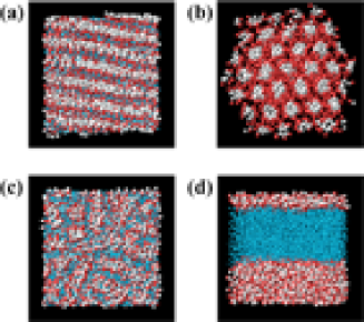
Figure 2: Formed structures for each potential coefficient, $x=-20(a),0(b),10(c),$ and $20(d).$ Each structure is shown in Table 2. Red and white beads denote hydrophilic (A) and hydrophobic molecules (B), respectively. Blue beads represent groups of water molecules (W). We set $T=0.5$ and $\phi=50\%$ during simulation.

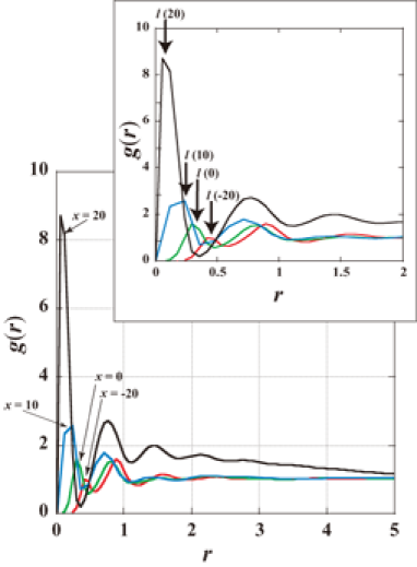
Figure 3: Solute particle radial distribution function $g(r)$ vs. distance between two particles $r$ for $x=-20,0,10$ and $20$. The function $g(r)$ is the sum of the A-A radial distribution function, the B-B radial distribution function, and the A-B radial distribution function. The first peak $l(x)$ of each curve corresponds to the length of AB dimer.

$x$	${\rm FormedStructures}$
-20	Lα
0	H1
10	L1
20	Phase separation

Table 2: Table of formed structures for each $x$. Lamellar, hexagonal, and micelles phases are indicated as L${}_{\rm\alpha},$ H${}_{1},$ and L${}_{1},$ respectively. For $x=20,$ AB molecules and W molecules are separated, as shown in Fig. 2.

References

- [1] D. J. Mitchell, G. J. T. Tiddy, L. Waring, Phase behaviour of polyoxyethylene surfactants with water, J. Chem. Soc., Faraday Trans. 1 79 (1983) 975.
- [2] T. Kato, Microstructure of nonionic surfactants, Structure-Performance Relationships in Surfactants 72 (1997) 325–357.
- [3] D. J. M. J. Israelachvili, B. W. Ninham, J. Chem. Soc. Faraday Trans. I 72 (1976) 1525.
- [4] J. Israelachvili, Intermolecular and Surface Forces, 2nd Edition, Academi Press, London, 1992.
- [5] P. J. Hoogerbrugge, J. M. V. A. Koelman, Simulating microscopic hydrocynamic phenomena with dissipative particle dynamics, Europhys. Lett. 19 (1992) 155.
- [6] R. D. Groot, P. B. Warren, Dissipative Particle Dynamics: Bridging the gap between atomistic and mesoscopic simulation, J. Chem. Phys. 107 (1997) 4423.
- [7] R. D. Groot, T. J. Madden, Dynamic simulation of diblock copolymer microphase separation, J. Chem. Phys. 108 (1998) 8713.
- [8] R. D. Groot, K. L. Rabone, Mesoscopic simulation of cell membrane damage, morphology change and rupture by nonionics surfactants, Biophys. J. 81 (2001) 725.
- [9] S. Jury, P. Bladon, M. Cates, S. Krishna, M. Hagen, N. Ruddock, P. Warren, Simulation of amphiphilic mesophases using dissipative particle dynamics, Phys. Chem. Chem. Phys. 1 (1999) 2051.
- [10] H. Nakamura, Mol. Simu. (2004) in press.
- [11] P. Español, P. Warren, Statistical mechanics of dissipative particle dynamics, Europhys. Lett. 30 (1995) 191.