Polarized networks, diameter, and synchronizability of networks

Abstract

Previous research claimed or disclaimed the role of a small diameter in the synchronization of a network of coupled dynamical systems. We investigate this connection and show that it is two folds. We first construct two classes of networks, the polarized networks and the random networks with a fixed diameter, which exhibit very different synchronizability. This shows that the diameter itself is insufficient to determine the synchronizability of networks. Secondly, we derive analytic estimates on the synchronizability of networks in terms of the diameter, and find that a larger size of network admits of a more flexible synchronizability. The analysis is confirmed by numerical results.

I Introduction

Since some critical properties of complex networks were revealed pioneerwork , both theoretical and experimental investigations of complex networks have received rapidly increasing interests review . After earlier verification of certain characteristics in various computer-generated and real-world networks verify , the focus of research shifted to the dynamics on complex networks sync . The synchronization of a network of dynamical systems has been extensively analyzed and has found many applications in secure communication, distance detection, and other engineering problems eng .

It is now well known that the synchronizability of a network can be characterized by the Laplacian spectrum of its associated graph. Consider a network of coupled dynamical systems $\dot{\mathbf{x}}^{i}=\mathbf{F}(\mathbf{x}^{i})+\sigma\sum_{j=1}^{n}L_{ij}\mathbf{H}(\mathbf{x}^{j})$, where $\mathbf{x}^{i}$ are the variables associated with node $i$; $\mathbf{F}$ and $\mathbf{H}$ are evolution and output functions, respectively; $\sigma$ is control strength; and $L_{ij}$ are entries of the Laplacian matrix, defined by $L_{ii}=k_{i}$, the degree of node $i$, $L_{ij}=-1$ if nodes $i$ and $j$ are connected, and $L_{ij}=0$ otherwise. Order the eigenvalues of the Laplacian matrix as $0=\lambda_{1}<\lambda_{2}\leq\cdots\leq\lambda_{n}$. Then, the larger the two quantities $\lambda_{2}$ and $\lambda_{2}/\lambda_{n}$ are, the better synchronizability the network exhibits sync ; sync-eig . However, the Laplacian eigenvalues provide little insights into how the network topology affects the dynamics of synchronization. Thus, it is important and useful to investigate the connection between the synchronizability of networks and some intuitive graph invariants. Since the degree sequence plays a central role in revealing the scale-free property of networks, its link with synchronizability has recently been studied degree . It was found that the degree sequence itself is unable to determine the synchronizability of networks, although it does provide efficient information under certain homogeneity constraints homo . The diameter, which is defined to be the maximal length of the shortest paths between any two vertices, has straightforward implication on the structure of a graph. Some previous experimental studies suggested that a small diameter might be advantageous to synchronization. This seems quite reasonable at the first sight, since a small diameter reduces the distance of signal transmission on the network, but lacks theoretical verification.

The purpose of this paper is to clarify the connection between the diameter and the synchronizability of networks. Instead of using experimental methods directly, we employ both constructions and analytic estimations. We first explicitly construct a class of determinate networks, named polarized networks, which keeps the diameter invariant while the network size increases. Inequalities in spectral graph theory are used to show that $\lambda_{2}$ and $\lambda_{2}/\lambda_{n}$ approach zero as the network size increases to infinity, and thus these networks are poorly synchronizable. Then, we use Erdős–Rényi random graph model erdos59 to obtain a class of random networks with the same diameter, whose synchronizability proves to be quite good. These facts are somewhat surprising, since they point out that the diameter may not be an appropriate quantity to characterize the synchronizability of networks. To make this observation consistent with those experiments that suggested the advantage of a small diameter, we further explore the role that the diameter plays in the synchronization of networks. Analytic estimates on the synchronizability of networks in terms of the diameter are derived and show that the diameter does set lower and upper bounds for networks of a certain size. By these estimates, we find that the synchronizability becomes more flexible as the network size increases. We also present numerical results that support the theoretical analysis.

II Network Constructions

In this section, we construct two classes of networks with prescribed diameter but very different synchronizability. To do this, we first recall some concepts in graph theory graph . A complete graph is a graph with no loops in which each pair of vertices are joined by one edge. The complete graph of order $n$ is denoted by $K_{n}$. Let $A$ and $B$ be two subsets of $V(G)$, the vertex set of graph $G$, and define the distance between $A$ and $B$ to be the minimal length of all paths between a vertex in $A$ and a vertex in $B$.

II.1 Networks with Poor Synchronizability

Suppose the network size $n$ and the diameter $D$ are given. We construct the polarized networks $P(n,D)$ by joining two complete graphs $K_{\left\lfloor\frac{n-D+3}{2}\right\rfloor}$ and $K_{\left\lceil\frac{n-D+3}{2}\right\rceil}$ by a path of length $D-2$; an example is shown in Fig. 1. It is easy to see that $P(n,D)$ has size $n$ and diameter $D$. Note that the orders of the two complete graphs differ by at most one, and they are highly clustering at the ends of a single path, from which the word “polarized” comes.

Figure 1: An example of polarized networks: $P(26,5)$. Two complete graphs $K_{12}$ are joined by a path of length 3.

To derive an upper bound on the second smallest Laplacian eigenvalue $\lambda_{2}$ of $P(n,D)$, we need a result in alon85 . If $A$ and $B$ are two subsets of $V(G)$ with distance $\rho$, and $F$ is the set of edges with at least one end vertex not in $A$ or $B$, then we have the lower bound on the order of $F$:

$$|F|\geq\rho^{2}\lambda_{2}\frac{|A||B|}{|A|+|B|}.$$ (1)

Now let $A$ and $B$ be the vertex sets of the two complete graphs in the construction of $P(n,D)$. Then clearly, we have $|A|=\left\lfloor\frac{n-D+3}{2}\right\rfloor$, $|B|=\left\lceil\frac{n-D+3}{2}\right\rceil$, $|F|=D-2$, and $\rho=D-2$. It follows from (1) that

$$\lambda_{2} \leq \frac{|F|(|A|+|B|)}{\rho^{2}|A||B|}=\frac{n-D+3}{(D-2)\left\lfloor\frac{n-D+3}{2}\right\rfloor\left\lceil\frac{n-D+3}{2}\right\rceil}$$ (4)

$$= \left\{\begin{array}[]{ll}\displaystyle\frac{4(n-D+3)}{(D-2)(n-D+2)(n-D+4)},&n-D\textrm{ even}\\ \displaystyle\frac{4}{(D-2)(n-D+3)},&n-D\textrm{ odd}\end{array}\right.$$

$$\leq \frac{4}{(D-2)(n-D+3)}.$$ (5)

On the other hand, a lower bound on the largest Laplacian eigenvalue $\lambda_{n}$ of a graph was given in fiedler73 . Let $\Delta$ be the maximal degree of a graph of order $n$. Then

$$\lambda_{n}\geq\frac{n}{n-1}\Delta.$$

Now in $P(n,D)$, $\Delta=\left\lceil\frac{n-D+3}{2}\right\rceil$. Therefore,

$$\lambda_{n}\geq\frac{n}{n-1}\left\lceil\frac{n-D+3}{2}\right\rceil\geq\frac{n(n-D+3)}{2(n-1)}.$$ (6)

Combining (5) and (6) gives

$$\frac{\lambda_{2}}{\lambda_{n}}\leq\frac{8(n-1)}{(D-2)\,n\,(n-D+3)^{2}}.$$ (7)

Letting $n\rightarrow\infty$ in (5) and (7) yields that both $\lambda_{2}$ and $\lambda_{2}/\lambda_{n}$ approach zero, which implies that the synchronizability of polarized networks can be arbitrarily poor as the network size increases. What is more, we will show in the next section that the polarized networks are nearly the optimal class of networks with poorest synchronizability among all the networks with the same network size and diameter.

II.2 Networks with Good Synchronizability

Instead of explicitly constructing a determinate network, we construct a class of random networks based on Erdős–Rényi random graph model. By this construction, we show that although there exist some extremal cases like the polarized networks, a general class of networks has fairly good synchronizability.

A random graph $G(n,p)$ consists of $n$ vertices and the edges chosen independently with probability $p$. For the purpose of our construction, we need to fix the diameter of the graphs for all network size $n$. However, the diameter of $G(n,p)$ may vary when $n$ increases, depending on how we choose $p$ as a function of $n$. Thus, we need a result concerning the diameter of $G(n,p)$ bollobas01 . Suppose the functions $D=D(n)\geq 3$ and $0<p=p(n)<1$ satisfy that $\log n/D-3\log\log n\rightarrow\infty$, $p^{D}n^{D-1}-2\log n\rightarrow\infty$, and $p^{D-1}n^{D-2}-2\log n\rightarrow-\infty$. Then $G(n,p)$ almost surely, i.e. with probability tending to one as $n$ tends to infinity, has diameter $D$. Here, let $D\geq 3$ be a constant and

$$p=\frac{(\alpha\,n\log n)^{1/(D-\varepsilon)}}{n}$$ (8)

where $0<\varepsilon<1$ and $\alpha$ can be any positive number. It is easy to verify that all the conditions mentioned above are satisfied, which yields that a random graph $G(n,p)$ with $p$ defined in (8) almost surely has diameter $D$.

The random graphs have a very narrow degree distribution. In fact, we have the proposition krivelevich05 , saying that if $p=p(n)$ satisfies that $pn/\log n\rightarrow\infty$ and $(1-p)\,n\log n\rightarrow\infty$, then almost surely all the degrees of $G(n,p)$ are equal to $(1+o(1))np$. It is clear that the assumptions are satisfied under (8). Hence, almost surely all the degrees of $G(n,p)$ with (8) holding are near $np$.

Now we are concerned with the Laplacian eigenvalues associated with $G(n,p)$. The Laplacian $L$ and the adjacency matrix $A$ of a graph are linked by the relation $L=K-A$, where $K$ is the diagonal matrix with diagonal entries being the vertex degrees. Due to the narrow distribution of degrees in $G(n,p)$, we have that $L\simeq npI-A$, and so

$$\lambda_{i}\simeq np-\bar{\lambda}_{i},\quad i=\overline{1,n},$$ (9)

where $\bar{\lambda}_{i}$ denote the eigenvalues of $A$. Therefore, what we need to know is the distribution of eigenvalues of the adjacency matrix $A$. We know that this distribution follows a semicircle law wigner , and a further result concerning all the eigenvalues $\bar{\lambda}_{i}$ except $\bar{\lambda}_{1}$ furedi81 says that

$$\max_{2\leq i\leq n}\left|\bar{\lambda}_{i}(G(n,p))\right|=O(\sqrt{np}).$$ (10)

And also notice that $\bar{\lambda}_{1}$ stands far away from the bulk of the spectrum, at $np$. Combining (9) and (10) yields

$$\lambda_{i}\simeq np+O(\sqrt{np}),\quad i=\overline{2,n}.$$

With (8), we obtain the approximations for the two quantities characterizing the synchronizability

$$\lambda_{2}\simeq np=(\alpha\,n\log n)^{1/(D-\varepsilon)},$$ (11)

$$\frac{\lambda_{2}}{\lambda_{n}}\simeq\frac{np-O(\sqrt{np})}{np+O(\sqrt{np})},$$ (12)

which implies that $\lambda_{2}\rightarrow\infty$ and $\lambda_{2}/\lambda_{n}\rightarrow 1$ as $n\rightarrow\infty$. By this we have shown that the class of random networks we constructed keeps the diameter invariant but exhibits rather good synchronizability.

III Analytic Estimations

By the constructions given in the previous section, we see that the synchronizability of networks with the same diameter may differ significantly. They also suggest that the diameter should not be an appropriate quantity to characterize the synchronizability of networks, although this is somewhat conflictive with intuition. Naturally, one could ask whether or not there exists some relation between the diameter and the synchronizability. The answer is yes; we will now confirm this relation by deriving some estimates on the quantities $\lambda_{2}$ and $\lambda_{2}/\lambda_{n}$. These estimates are based on a series of inequalities in spectral graph theory.

A lower bound on $\lambda_{2}$ in terms of the network size $n$ and the diameter $D$ mohar91 pointed out that

$$\lambda_{2}\geq\frac{4}{nD}.$$ (13)

Chung chung94 estimated the diameter $D$ by giving the upper bound

$$D\leq\left\lfloor\frac{\cosh^{-1}(n-1)}{\cosh^{-1}\left(\frac{\lambda_{n}+\lambda_{2}}{\lambda_{n}-\lambda_{2}}\right)}\right\rfloor+1,$$

which implies that

$$D-1\leq\frac{\cosh^{-1}(n-1)}{\cosh^{-1}\left(\frac{1+\lambda_{2}/\lambda_{n}}{1-\lambda_{2}/\lambda_{n}}\right)}.$$

We can solve this inequality and obtain an upper bound on $\lambda_{2}/\lambda_{n}$

$$\frac{\lambda_{2}}{\lambda_{n}}\leq\frac{\cosh\left(\frac{\cosh^{-1}(n-1)}{D-1}\right)-1}{\cosh\left(\frac{\cosh^{-1}(n-1)}{D-1}\right)+1}.$$ (14)

Now note that a simple upper bound on $\lambda_{n}$ was given kelmans67 by

$$\lambda_{n}\leq n$$ (15)

with equality holding if and only if the complement of the graph is disconnected. Combining (13), (14), and (15) gives the estimates as follows.

Proposition: Given the network size $n$ and the diameter $D$, the following estimates on $\lambda_{2}$ and $\lambda_{2}/\lambda_{n}$ hold:

$$\frac{4}{nD}\leq\lambda_{2}\leq n\,\frac{\cosh\left(\frac{\cosh^{-1}(n-1)}{D-1}\right)-1}{\cosh\left(\frac{\cosh^{-1}(n-1)}{D-1}\right)+1},$$ (16)

$$\frac{4}{n^{2}D}\leq\frac{\lambda_{2}}{\lambda_{n}}\leq\frac{\cosh\left(\frac{\cosh^{-1}(n-1)}{D-1}\right)-1}{\cosh\left(\frac{\cosh^{-1}(n-1)}{D-1}\right)+1}.$$ (17)

Proof: The upper bound on $\lambda_{2}$ follows from (14) and (15), and the lower bound on $\lambda_{2}/\lambda_{n}$ follows from (13) and (15). $\Box$

To gain more insights into the connection between the diameter and the synchronizability, we find an asymptotic order of the upper bound on $\lambda_{2}/\lambda_{n}$. It is easy to calculate that

$$\frac{\cosh\left(\frac{\cosh^{-1}(n-1)}{D-1}\right)-1}{\cosh\left(\frac{\cosh^{-1}(n-1)}{D-1}\right)+1}\simeq\frac{(2n)^{1/(D-1)}-2}{(2n)^{1/(D-1)}+2}.$$

With the estimates and asymptotic order, it is easily seen that a larger diameter $D$ implies both smaller lower bounds and smaller upper bounds on $\lambda_{2}$ and $\lambda_{2}/\lambda_{n}$. This observation coincides with the intuition that a larger diameter is likely to be harmful to synchronization. From this point of view, the assertion that a small diameter benefits synchronization could be true, although it is not true for individual networks.

Another observation worthwhile to point out is that a larger network size $n$ implies smaller lower bounds and larger upper bounds on both $\lambda_{2}$ and $\lambda_{2}/\lambda_{n}$. In other words, the synchronizability of networks becomes more flexible as the network size increases. This fact suggests that the indicator role of the diameter in synchronization will substantially weaken in large-size networks.

Let us return to the polarized networks for which the estimates on $\lambda_{2}$ and $\lambda_{2}/\lambda_{n}$ were given in (5) and (7), respectively. The asymptotic orders of the upper bounds are $4/(nD)$ and $8/(n^{2}D)$, respectively, for large $n$ and $D$, and $n\gg D$. Thus, by the Proposition, we see that the polarized networks are almost the optimal class of networks with poorest synchronizability.

IV Numerical Results

In this section, we carry out numerical experiments to explore the connection between the diameter and the synchronizability for the two classes of networks we constructed. Note that the polarized networks are determinate while the random networks are, of course, not. So the former case is much simpler, while some average methods should be used to eliminate random perturbations in the latter case.

In the polarized networks, all we need to determine before generating the network topology are the network size $n$ and the diameter $D$. To investigate the influence of network size $n$ and diameter $D$ on the synchronizability of polarized networks, we assigned a set of values to the two parameters, and plotted the trends of the two quantities that characterize the synchronizability in Figs. 2 and 3. According to the lower bound estimates in (16) and (17), combined with the upper bound estimates in (5) and (7), the relationships between the pairs of parameters we have shown in Figs. 2 and 3 are expected to be all linear. The numerical results are quite consistent with and support this observation. They confirm that the synchronizability of polarized networks is very poor, and decreases toward zero at least linearly as the networks size and diameter increase.

Figure 2: The relationships between the network size $n$ and the two quantities that characterize the synchronizability of polarized networks $P(n,D)$. The diameter $D$ is set to 5 all the time.

Figure 3: The relationships between the diameter $D$ and the two quantities that characterize the synchronizability of polarized networks $P(n,D)$. The network size $n$ is set to 200 all the time.

Now we turn to the random networks $G(n,p)$ with $p$ defined in (8). It is worth noticing that although any $0<\varepsilon<1$ and $\alpha>0$ ensure the convergence of diameter to the specified value, a careful selection of their values will accelerate the convergence so that networks with a particular diameter may be obtained for relatively small network sizes. In our experiments, we always set $\varepsilon=0.5$, but choose different $\alpha$ values for different diameters $D$. The results of experiments for $D=4$ and $\alpha=5$ are illustrated in Fig. 4. In the experiments, ten random networks were generated for each network size $n$, and the averages of $\lambda_{2}$ and $\lambda_{2}/\lambda_{n}$ were computed respectively. The diameter converged fast to and stayed stably at the specified value. This is shown in the bottom of Fig. 4, where $N$ denotes the number of networks achieving diameter $D$ out of the ten for each network size $n$. Meanwhile, the two quantities $\lambda_{2}$ and $\lambda_{2}/\lambda_{n}$ related to the synchronizability went up slowly. These trends are in agreement with the analytic estimations. However, it is difficult to obtain the accurate growing speeds of the two quantities by numerical experiments, since the required computations increase very rapidly along with the network size.

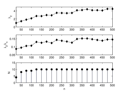
Figure 4: The performance of random networks with $p$ defined in (8). For the set of fixed parameters $D=4$, $\varepsilon=0.5$, $\alpha=5$, ten random networks were generated for each network size $n$. The averages of the two quantities related to the synchronizability are shown in the top two graphs, while $N$, the number of networks achieving diameter $D$ out of the ten for each network size $n$ is shown in the bottom.

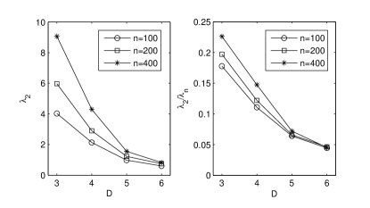
Figure 5: The average performance of the class of random networks we constructed, under different diameters and network sizes. Here $\varepsilon=0.5$, and $\alpha$ is set appropriately to ensure fast convergence to the specified diameter. For each set of parameters, 50 random networks were generated and averages of the two quantities related to the synchronizability were computed respectively.

More accurate numerical results are shown in Fig. 5, where 50 random networks were generated for each set of parameters and averages of $\lambda_{2}$ and $\lambda_{2}/\lambda_{n}$ were computed respectively, so that the effects of random perturbations could be reduced remarkably. First, it is clear that the increasing diameter has pulled down the synchronizability of networks. This is consistent with the intuitive observation that a large diameter would impede communications between nodes and synchronization in a certain class of random networks, although the observation is absolutely not true for determinate networks, for instance, a polarized network and a typical sample in the random networks with the same diameter, which have been shown to perform distinctly in synchronization.

Another observation which can be seen from Fig. 5 is that the class of random networks has an obvious trend in the improvement of synchronizability as the network size increases, which turns out to be the same as what has been confirmed by Fig. 4. However, it is worth noticing that this trend becomes quite faint for a large diameter. This can be seen from the asymptotic orders in (11) and (12). Restricted by the complexity of computation, we were only able to conduct the experiments in a relatively small range of network size $n$, but the increase of network size was pulled down considerably by a large diameter $D$, according to (11) and (12).

V Conclusions

We investigated the connection between the diameter and the synchronizability of networks. By constructing determinate polarized networks and a class of random networks, we found that the networks with the same diameter may have very different synchronizability. Thus, the diameter itself is inappropriate to be a quantity that characterizes the synchronizability of networks. We also derived analytic estimates on the range of synchronizability of networks with specified diameter and network size, which revealed that a larger size of network admits of a more flexible synchronizability.

An application of the network constructions is the design of network topology in communications, multi-agent systems, and other engineering problems. Since the polarized networks are almost the optimal class of networks with poorest synchronizability, they are especially suitable to be used in the design of easily desynchronizable networks. Moreover, the nature of explicit constructions makes it quite easy to apply. The random networks with fixed diameter are also useful in synchronization-related applications that have special requirements on the diameter of networks. The fast convergence to the specified diameter enables us to generate desired networks of relatively small sizes.

A noteworthy endeavor in the literature is to explicitly construct networks with best synchronizability. Recently, methods in numerical optimization such as simulated annealing have been utilized to obtain nearly optimal network topology donetti05 . It was suggested that the optimal network topology should possess several important properties, including homogeneous degree, betweenness, and distance distributions, large girths, small diameters, no community structure, etc. However, the procedure to generate such a network topology remains an open question. As pointed out in this paper and previous research, individual properties such as small diameters, homogeneous degree distributions, etc., are insufficient to optimize the synchronizability of networks. A successful constructing algorithm should instead take into account a full combination of these favorable properties.

References

- (1) D. J. Watts and S. H. Strogatz, Nature (London) 393, 440 (1998); A.-L. Barabási and R. Albert, Science, 286, 509 (1999).
- (2) S. H. Strogatz, Nature (London) 410, 268 (2001); R. Albert and A.-L. Barabási, Rev. Mod. Phys. 74, 47 (2002); M. E. J. Newman, SIAM Rev. 45, 167 (2003); S. Boccaletti et al., Phys. Rep. 424, 175 (2006).
- (3) H. Jeong et al., Nature (London) 407, 651 (2000); L. A. N. Amaral et al., Proc. Natl. Acad. Sci. U.S.A. 97, 11149 (2000); R. Pastor-Satorras, A. Vázquez, and A. Vespignani, Phys. Rev. Lett. 87, 258701 (2001).
- (4) X. F. Wang and G. Chen, Int. J. Bifurcation Chaos Appl. Sci. Eng. 12, 187 (2002); M. Barahona and L. M. Pecora, Phys. Rev. Lett. 89, 054101 (2002).
- (5) X. Li and G. Chen, IEEE Trans. Circuits Syst. I: Fundam. Theory Appl. 50 1381 (2003); W. Lu and T. Chen, Physica D 213, 214 (2006).
- (6) C. W. Wu and L. O. Chua, IEEE Trans. Circuits Syst. I: Fundam. Theory Appl. 42, 430 (1995); J. Jost and M. P. Joy, Phys. Rev. E 65, 016201 (2002); F. M. Atay, J. Jost, and A. Wende, Phys. Rev. Lett. 92, 144101 (2004); W. Lu and T. Chen, Physica D 198, 148 (2004).
- (7) F. M. Atay, T. Bıyıkoğlu, and J. Jost, IEEE Trans. Circuits Syst. I: Regular Papers 53, 92 (2006); C. W. Wu, Phys. Lett. A 346, 281 (2005).
- (8) T. Nishikawa, A. E. Motter, Y.-C. Lai, and F. C. Hoppensteadt, Phys. Rev. Lett. 91, 014101 (2003); F. Chung, L. Lu, and V. Vu, Proc. Natl. Acad. Sci. U.S.A. 100, 6313 (2003).
- (9) P. Erdős and A. Rényi, Publ. Math. (Debrecen) 6, 290 (1959).
- (10) R. Diestel, Graph Theory (Springer, Heidelberg, 2005), http:// www.math.uni-hamburg.de/home/diestel/books/graph.theory.
- (11) N. Alon and V. D. Milman, J. Combin. Theory, Ser. B 38, 73 (1985).
- (12) M. Fiedler, Czech. Math. J. 23, 298 (1973).
- (13) B. Bollobás, Random Graphs (Cambridge University Press, Cambridge, 2001), p. 263.
- (14) M. Krivelevich and B. Sudakov, e-print math.CO/0503745.
- (15) E. P. Wigner, Ann. Math. 62, 548 (1955); 67, 325 (1958).
- (16) Z. Füredi and J. Komlós, Combinatorica 1, 233 (1981).
- (17) B. Mohar, Graphs Combin. 7, 53 (1991).
- (18) F. R. K. Chung, V. Faber, and T. A. Manteuffel, SIAM J. Discrete Math. 7, 443 (1994).
- (19) A. K. Kel’mans, in Cybernetics—in the Service of Communism, Vol. 4 (Izdat. “Ènergija”, Moscow, 1967), pp. 27–41 (Russian).
- (20) L. Donetti, P. I. Hurtado, and M. A. Muñoz, Phys. Rev. Lett. 95, 188701 (2005).