Reaction kinetics of coarse-grained equilibrium polymers: a Brownian Dynamics study

0.1 Abstract

Self-assembled linear structures like giant cylindrical micelles or discotic molecules in solution stacked in flexible columns are systems reminiscent of polydisperse polymer solutions, ranging from dilute to concentrated solutions as the overall monomer density and/or the chain length increases. These supramolecular polymers have an equilibrium length distribution, the result of a competition between the random breakage of chains and the fusion of chains to generate longer ones. This scission-recombination mechanism is believed to be responsible of some peculiar dynamical properties like the Maxwell fluid rheological character for entangled micelles. Simulations employing simple mesoscopic models provide a powerful approach to test mean-field theories or scaling approaches which have been proposed to rationalize the structural and kinetic properties of these soft matter systems. In the present work, we review the basic theoretical concepts of these “equilibrium polymers” and some of the important results obtained by simulation approaches. We propose a new version of a mesoscopic model in continuous space based on the bead and FENE spring polymer model which is treated by Brownian Dynamics and Monte-Carlo binding/unbinding reversible changes for adjacent monomers in space, characterized by an attempt frequency parameter $\omega$. For a dilute and a moderately semi-dilute state-points which both correspond to dynamically unentangled regimes, the dynamic properties are found to depend upon $\omega$ through the effective life time $\tau_{b}$ of the average size chain which, in turn, yields the kinetic reaction coefficients of the mean-field kinetic model proposed by Cates. Simple kinetic theories seem to work for times $t\geq\tau_{b}$ while at shorter time, strong dynamical correlation effects are observed. Other dynamical properties like the overall monomer diffusion and the mobility of reactive end-monomers are also investigated.

0.2 Introduction

In the field of self-assembling structures, supramolecular polymers are attracting nowadays much attention VdS . It is well known and schematically illustrated in figure 1 that some surfactant molecules in solution can self-assemble and form wormlike micelles catc .

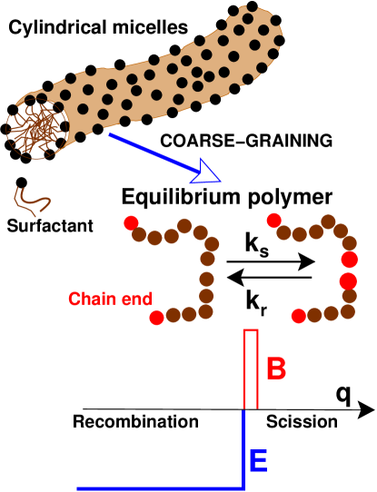
Figure 1: Some surfactant molecules in solution self-assemble and form long wormlike micelles which continously break and recombine.Their mass distribution is, hence, in thermal equilibrium and they present an important example of the vaste class of systems termed “equilibrium polymers”VdS .The free energy $E$ of the (spherical) end cap of these micelles has been estimated catc to be of order of $10k_{B}T$. This energy penalty (together with the monomer density) determines essentially the static properties and fixes the ratio of the scission and recombination rates, $k_{s}$ and $k_{r}$. Additionally, these rates are influenced by the barrier height $B$ which has been estimated to be similar to the end cap energy. Both important energy scales have been sketched schematically as a function of a generic reaction coordinate $q$ (see chapter 8 of reference chand ).Following closely the analytical description catc ; witt98 these micellar systems are represented in this study by coarse-grained effective potentials in terms of a standard bead-spring model. The end cap free energy becomes now an energy penalty for scission events, i.e., the creation of two unsaturated chain ends. The dynamical barrier is taken into account by means of an attempt frequency $\omega=\exp{(-B/k_{B}T)}$. If $\omega$ is large, successive breakage and recombination events for a given chain can be assumed to be uncorrelated and the recombination of a newly created chain ends will be of standard mean-field type. On the other hand, the (return) probability that two newly created chain ends recombine immediately must be particulary important at large $\omega$. These highly correlated “diffusion controlled” oshau recombination events do not contribute do the effective macroscopic reaction rates which determine the dynamics of the system. The key task of this paper is to compare different methods to compute the effective rates as a function of the attempt frequency $\omega$ for a weakly semi-dilute state point in the non-entangled dynamical regime.

Such micellar solutions exhibit fascinating rheological behaviour, such as shear-bandingleroug , shear-thickenninghoff , Maxwell fluid behaviour catc or anomalous diffusion (Levy flight)OBL90 . Self-assembled stacks of discotic molecules and chains of bifunctional molecules are other examples of supramolecular polymers. All these examples differ by the nature of the intermolecular forces involved in the self-assembling of the basic units, but they lead to a similar physical situation bearing much analogy with a traditional system of polydisperse flexibles polymers when their length becomes sufficiently large with respect to their persistence length. The specificity and originality of these supramolecular polymers comes from the fact that these chains are continuously subject to scissions at random places along their contour and subject to end to end recombinations, leading to a dynamical equilibrium between different chain lengths species. These supramolecular polymers are typical soft matter systems and the chain length distribution which determines their properties, is very sensitive to external conditions (temperature, concentration, external fields, salt contents, etc…).

Different times scales and length scales are involved in these systems, as in usual polymer systems. Unlike the latter, which have been much studied during the last 50 yearsgennes ; GK94 ; doi , theoretical work on micellar solutions are quite recentVdS ; catc . While building up a molecular scale theory is clearly too heavy for such complex systems, theoretical approaches, based on mean-field concept and non-local phenomenological approaches, can explore with success some equilibrium, and rheological propertiescates ; spen ; olms , under reasonable but often drastic approximations. Concerning specifically micelle kinetics, recently, O’Shaughnessy and Yu oshau suggested that there are two possible kinds of kinetics associated with scission/recombination: diffusion controlled and mean-field, which may be distinguished by the time dependence of the first recombination times distribution function of the chains.

In parallel, mesoscopic scale computer simulations can shed much light on these rich but complex systems, thanks to techniques borrowed from simulations of polymers. Systems of wormlike micelles can be modelled by “Equilibrium polymers” (EP), sometimes called “living polymers”, which are polymer chains endowed with scission/recombination (S-R) processes taking place in them. The advantage of numerical studies is their ability to make links either to experiments or to mean-field type theories, given that those systems are difficult to characterize by experiments and the results are not simple to interpret. The bond fluctuation model (BFM) has been the object of intensive studies on the statics and dynamics of living polymerswitt98 ; milch .

Brownian dynamics studies of a similar model rouau have been used to study the scaling predictions on the dependence of the average chain length upon the overall monomer density. In a recent study, Padding and Boekpadd showed that a mesoscopic model of wormlike micelle known as the FENE-C modelkrog , seems to obey the diffusion-controlled kinetics.

In our workhuang which is the basis for this course, we investigate the structural and kinetic properties of equilibrium polymers in solution by means of a Brownian Dynamics algorithm applied to a standard polymer modelkrem coupled to a time-reversible EP algorithm for polymer scission-recombinations witt98 ; milch ; MWL99 ; MW01 ; WM00 . This particular continuous space model has the advantage that its kinetic properties are well separated from the structural and thermodynamical aspects. Our model does not allow for cyclic structures and hence, we simplify the computational load and, more importantly, the theoretical interpretation of the static and dynamical properties of our samples. Anyway, for cylindrical micelles, cyclic structures are expected to exist in very low concentrations catc .

We study the kinetics of equilibrium polymers solutions at two state points, exploring in each case a range of rates of the scission-recombination process. The two state points correspond to a dilute solution and a semi-dilute solution regime close to the cross-over region. A direct measure of chain overlap can be provided by the ratio of the mean distance between chain centres of mass over the radius of giration of the average size chain (respectively $\approx 10$ and $\approx 50$ for the dilute and semi-dilute cases). This gives ratios of $1.4$ for the dilute case and $0.6$ for the semi-dilute case, which suggests that even in the semi-dilute case, the chain relaxation is still typically Rouse like and thus yet kinetically entangled.

The main focus is to link the microscopic model to the more macroscopic kinetics theories, e.g. by Cates catc , and to discuss in a well defined case the concepts of ’diffusion controlled’ and ’mean-field’, defined by authors ofoshau ; padd . In particular, we want to estimate the effective reaction rates for the scission and recombination processes comparing different methods. Furthermore, we shall study the diffusion of monomers and discuss their link to the scission/recombination kinetics.

0.3 Theoretical framework

0.3.1 Statistical mechanics derivation of the distribution of chain lengths

To treat a system of supramolecular polymers theoretically, it is convenient to work at the mesoscopic scale using a model of linear flexible polymers made of L monomers of size $b$ linked together by a non permanent bonding scheme. Within the system, individual chain lengths fluctuate by bond scission and by fusion of two chain ends of different chains. Statistical mechanics can be employed to predict the equilibrium distribution of chain lengthscatc . In terms of the equilibrium chain number density $c_{0}(L)$, the average chain length $L_{0}$ and the total monomer density $\phi$ are given by

$$L_{0}=\frac{{\sum_{L=0}^{\infty}}Lc_{0}(L)}{\sum_{L=0}^{\infty}c_{0}(L)}$$ (1)

$$\phi=\sum_{L=0}^{\infty}Lc_{0}(L)=\frac{M}{V}$$ (2)

where $M$ denotes the total number of monomers in the system.

Conceptually, we consider the Helmholtz free energy $F(V,T;\{N(L)\},N_{s})$ of a mixture of chains molecules of different length $L$ in solvent where, in addition to the temperature T, the volume V and the number of solvent molecules $N_{s}$, the number of chains of each specific length $N(L)$ is fixed. Let $F(V,T;M,N_{s})$ be the Helmholtz free energy of a similar system where only the total number of solute monomers $M$ is fixed. The equilibrium chain length distribution $c_{0}(L)=N(L)/V$ will result from the set $\{N(L)\}$ which satisfies the condition

$$F(V,T;M,N_{s})=min_{\{N(L)\}}\left[F(V,T;\{N(L)\},N_{s})+\mu\sum_{L=0}^{\infty}LN(L)\right]$$ (3)

The parameter $\mu$ is the Lagrange multiplier associated with the constraint that individual numbers of chains $N(L)$ must keep fixed the total number of monomers $M=\sum_{0}^{\infty}LN(L)$. Minimisation requires that the first derivative with respect to any $N(L^{\prime})$ variable (L’=1,2, …) is zero, giving

$$\frac{\delta F(V,T;\{N(L)\},N_{s})}{\delta N(L^{\prime})}+\mu L^{\prime}=0;L^{\prime}=1,2,...$$ (4)

We expect the entropic part of the total free energy $F(V,T;\{N(L)\},N_{s})$ to be the sum of translational and chain internal configurational contributions which both depend upon the way the M monomers are arranged into a particular chain size distribution. For the translation part, the polydisperse system entropy is estimated as the ideal mixture entropy $S_{id}$

$$S_{id}(V,T;\{N(L)\},N_{s})=-k_{B}\sum_{L}N(L)\ln{(CN(L))}+S^{solv}$$ (5)

where $C=b^{3}/V$ is a dimensionless constant independent of L and where $S^{solv}$ is the solvent contribution, independent of the $N(L)$ distribution. The configurational entropy of an individual chain with L monomers is written as $S_{1}(L)=k_{B}\ln{\Omega_{L}}$, in terms of $\Omega_{L}$, the total number of configurations of the chain. Adding the configurational contributions to $S_{id}$ as given by eq.(5), the total entropy becomes

$$S(V,T;\{N(L)\},N_{s})=-k_{B}\sum_{L}N(L)\left[\ln{(CN(L))}-\ln{\Omega_{L}}\right]+S^{solv}$$ (6)

We now turn to the energy $E(V,T;\{N(L)\},N_{s})$ of the same system. If $E_{1}(V,T;\\ L)$ represents the internal energy of a chain of $L$ monomers and $E_{s}$ the energy of a solvent molecule, the energy can be written as

$$E(V,T;\{N(L)\},N_{s})=\sum_{L}N(L)E_{1}(V,T;L)+N_{s}E_{s}(V,T)$$ (7)

The key contribution in $E_{1}$ is the chain end-cap energy $E$ which corresponds to the chain end energy penalty required to break a chain in two pieces. We will suppose that $E_{1}(L)=E+L\tilde{\epsilon}$ where $\tilde{\epsilon}$ is an irrelevant energy per monomer as $M\tilde{\epsilon}$, its total contribution to the system energy, is independent of the chain length distribution.

The present approximation of the total free energy of the system is thus given by incorporating in the general expression (3) the expressions (6) and (7), giving

$$\beta F(V,T;\{N(L)\},N_{s})=\sum_{L}N(L)\left[\ln{N(L)}+\ln{C}-\ln{\Omega_{L}}+\beta E+\beta\tilde{\epsilon}L\right]$$ (8)

where irrelevant constant solvent terms have been omitted as we only need the first derivative of the free energy with respect to $N(L)$, which now takes the form

$$\frac{\delta\beta F}{\delta N(L)}=\ln{N(L)}+\ln{C}-\ln{\Omega_{L}}+\beta E+\beta\tilde{\epsilon}L+1.$$ (9)

With this expression, the minimisation condition on $N(L)$ becomes

$$\ln{N(L)}+\ln{C}-\ln{\Omega_{L}}+\beta E+1+\mu^{\prime}L=0$$ (10)

where $\mu^{\prime}=(\beta\mu+\beta\tilde{\epsilon})$. We note at this stage that the second derivative of $\beta F(V,T;\\ \{N(L)\})+\mu^{\prime}\sum_{L}LN(L)$ with respect to $N(L)$ and $N(L^{\prime})$ variables gives the non negative result $\frac{\delta_{LL^{\prime}}}{N(L)}$, indicating that the extremum is indeed a minimum.

Solving for $N(L)$ in eq.(10), we get

$$N(L)={C^{\prime}}^{-1}\exp{-(\mu^{\prime}L+\beta E-\ln{\Omega_{L}})}$$ (11)

where $C^{\prime}=eC$ while, according to eq. (2)), $\mu^{\prime}$ must be such that

$$\sum_{L}L\exp{-(\mu^{\prime}L+\beta E-\ln{\Omega_{L}})}=MC^{\prime}$$ (12)

The equilibrium $N(L)$ variables are also related to the equilibrium chain length average $L_{0}$ (see eq. (1)), so that

$$\sum_{L}\exp{-(\mu^{\prime}L+\beta E-\ln{\Omega_{L}})}=\frac{MC^{\prime}}{L_{0}}$$ (13)

To progress, we now need to specify the explicit $L$ dependence of $\Omega_{L}$. The traditional single chain theories of polymer physics provide universal expression of $\Omega_{L}$ in terms of the polymer size, the environment being simply taken into account through the solvent quality and the swollen blob size in the semi-dilute (good solvent) case.

The case of mean field or ideal chains

The basic mean-field or ideal chain model for a L segments chain gives

$$\Omega_{L}^{id}=\left[C_{1}z^{L}\right]$$ (14)

where $z$ is the single monomer partition function and $C_{1}$ a dimensionless constant. Adapting eq.(11), one has

$$N(L)=\frac{C_{1}}{C^{\prime}}\exp{-(\beta E)}\exp{(-\mu"L)}$$ (15)

where $\mu"=\mu^{\prime}-\ln{z}$ must, according to eq. (12), be such that

$$\sum_{L}L\exp{-(\mu"L)}=\frac{1}{\mu"^{2}}=\frac{MC^{\prime}}{C_{1}\exp{-(\beta E)}}$$ (16)

while eq.(13) takes the form

$$\sum_{L}\exp{-(\mu"L)}=\frac{1}{\mu"}=\frac{MC^{\prime}}{L_{0}C_{1}\exp{-(\beta E)}}$$ (17)

In eqs.(16) and (17), sums over $L$ from $1$ to $\infty$ have been approximated by the result of their continuous integral counterparts.

Combining eqs.(15), (16) and (17), one gets the final expression for the chain number densities

$$c_{0}(L)=\frac{\phi}{L_{0}^{2}}\exp{(-\frac{L}{L_{0}})}$$ (18)

with the average polymer length given by

$$L_{0}=B^{1/2}\phi^{\frac{1}{2}}\exp{\left(\frac{\beta E}{2}\right)}.$$ (19)

where $B=eb^{3}/C_{1}$ is a constant depending upon the monomer size $b$ and the prefactor in the number of ideal chain configurations in eq.(14).

The case of dilute chains in good solvent

Polymer solutions in good solvent are in a dilute regime when chains do not overlap and in semi-dilute regime when chains do strongly overlap while the total monomer volume fraction is still well below its melt value. In the semi-dilute regime, chains remain swollen locally over some correlation length, known as the swollen blob size $\chi$, but they are ideal over larger distances as a result of the screening of excluded volume interactions between blobs.

Specifically, for a given monomer number density $\phi$, the blob size is given by the condition that the blob volume times $\phi$ must be equal to the number of monomers $L^{*}$ in the swollen blob. This gives in terms of the reduced number density $\phi^{\prime}=b^{3}\phi$

$$L^{*} \sim {\phi^{\prime}}^{\left(\frac{1}{1-3\nu}\right)}$$ (20)

$$\chi \sim b{\phi^{\prime}}^{\left(\frac{\nu}{1-3\nu}\right)}$$ (21)

where $\nu=0.588$ in present good solvent conditionsdoi .

In living polymers characterized by a monomer number density $\phi$ and some averaged chain length $L_{0}$, the semi-dilute conditons correspond to the case $L_{0}>>L^{*}$. We discuss in this subsection the theory for the dilute case where $L_{0}<<L^{*}$. We will come back to the semi-dilute case in the next subsection.

Self-avoiding walks statistics apply to dilute chains in good solvent, and we thus adopt the number of configurationsgennes ; GK94 (See especially page 128 of the book of Grosberg and KhokhlovGK94 )

$$\Omega_{L}^{EV}=C_{1}L^{(\gamma-1)}z^{L}$$ (22)

where $\gamma$ is the (entropy related) universal exponent equal to $1.165$.

Incorporating expression (22) in eq. (11), one gets

$$N(L)=\frac{V}{B}\exp{-(\beta E)}L^{(\gamma-1)}\exp{-(\mu"L)}$$ (23)

where $B$ was introduced in eq.(19) and where $\mu"=\mu^{\prime}-\ln{z}$ must be fixed by eq.(2)

$$\sum_{L}L^{\gamma}\exp{-(\mu"L)}=B\phi\exp{(\beta E)}$$ (24)

while eq.(13) takes here the form

$$\sum_{L}L^{(\gamma-1)}\exp{-(\mu"L)}=\frac{B\phi}{L_{0}}\exp{(\beta E)}$$ (25)

If $L$ is treated as a continuous variable, eqs(24) and (25) can be rewritten in terms of the Euler Gamma function satisfying $\Gamma(x)=x\Gamma(x-1)$ as

$$\int_{0}^{\infty}L^{\gamma}\exp{-(\mu"L)}dL=\frac{\Gamma(\gamma+1)}{\mu"^{(\gamma+1)}}=B\phi\exp{(\beta E)}$$ (26)

$$\int_{0}^{\infty}L^{(\gamma-1)}\exp{-(\mu"L)}dL=\frac{\Gamma(\gamma)}{\mu"^{\gamma}}=\frac{B\phi}{L_{0}}\exp{(\beta E)}$$ (27)

From eqs (26) and (27), one gets

$$\mu" = \frac{\gamma}{L_{0}}$$ (28)

$$B\phi\exp{(\beta E)} = \frac{\Gamma(\gamma+1)}{\gamma^{(\gamma+1)}}L_{0}^{(\gamma+1)}$$ (29)

These results lead then finally to the Schulz-Zimm distribution of chain lengths, namely

$$c_{0}(L)=\frac{\exp{(-\beta E)}}{B}L^{(\gamma-1)}\exp{(-\gamma\frac{L}{L_{0}})}$$ (30)

and an average polymer length given by

$$L_{0}=\left(\frac{\gamma^{\gamma}}{\Gamma(\gamma)}\right)^{\frac{1}{1+\gamma}}B^{\frac{1}{1+\gamma}}\phi^{\frac{1}{1+\gamma}}\exp{\left(\frac{\beta E}{(1+\gamma)}\right)}.$$ (31)

The semi-dilute case

We consider here the semi-dilute case in good solvent where the average length of living polymers $L_{0}$ is much larger than the blob length $L^{*}$. The usual picture of a semi-dilute polymer solution is an assembly of ideal chains made of blobs of size $\chi$. Using this approach, Cates and Candau catc and later J.P. Wittmer et al witt98 derived the relevant equilibrium polymer size distribution. In this subsection, we adapt their derivation to the theoretical framework presented above.

Let $\Omega_{b}$ be the number of internal configurations per blob and $z^{\prime}$ some coordination number for successive blobs. As there are $n_{b}=L/L^{*}$ blobs for a chain of L monomers, we write the total number of internal configurations of a chain of size L as

$$\Omega_{L}^{SD}=C_{1}L^{*(\gamma-1)}\Omega_{b}^{L/{L^{*}}}{z^{\prime}}^{L/{L^{*}}}$$ (32)

where $\gamma$ is the universal exponent in the excluded volume chain statistics met earlier for chains in dilute solutions. The important factor $L^{*(\gamma-1)}$ can be seen as an entropy correction for chain ends just like $E$ was an energy correction to $L\tilde{\epsilon}$. This entropic term which involves the number of monomers per blob, is needed to take into account that when a chain breaks, its two ends are subject to a reduced excluded volume repulsion. The other factors in eq.(32) will lead to terms linear in $L$ after taking the logarithm and thus will be absorbed in the Lagrange multiplier definition, as seen earlier in similar cases for ideal and dilute chains.The resulting expression of $N(L)$ in terms of the Lagrange multiplier (cfr eq.(15)) can then be written by analogy as

$$N(L)=\frac{C_{1}}{C^{\prime}}\exp{-\left[\beta E-(\gamma-1)\ln{L^{*}}\right]}\exp{(-\mu L)}$$ (33)

Proceeding as in the ideal case (simply replacing at every step the constant $\beta E$ by $\beta E-(\gamma-1)\ln{L^{*}}$, one recovers in the semi-dilute case the simple exponential distribution

$$c_{0}(L)=\frac{\phi}{L_{0}^{2}}\exp{(-\frac{L}{L_{0}})}$$ (34)

with a slightly different formula for the average polymer length

$$L_{0}\propto\phi^{\alpha}\exp{\left(\frac{\beta E}{2}\right)}$$ (35)

where $\alpha=\frac{1}{2}(1+\frac{\gamma-1}{3\nu-1})$ is about 0.6.

0.3.2 A kinetic model for scissions and recombinations

The interest for wormlike micelles dynamics came from the experimental observation that entangled flexible supramolecular polymers display, after an initial strain, a simple exponential stress relaxation which is qualitatively different from the behaviour of usual entangled melts. In the latter system, individual chains must leave by a reptation mechanism the strained topological tube created by the entangled temporarily network, in order to relax the shearing forces. A plausible scission-recombination model, allowing for such an extra relaxation mechanism, was shown catc to lead to an exponential decay of the shearing forces with a decay Maxwell time equal to $\tau\approx\sqrt{\tau_{b}\tau_{rep}}$ where $\tau_{rep}$ is the chain reptation time and $\tau_{b}$ is the mean life time of a chain of average size in the system.

We will assume in the following that the Cate’s scission-recombination model governing the population dynamics, originally deviced to explain entangled equilibrium polymer melt rheology, should also apply to the kinetically unentangled regime which is explored in the present work.

This kinetic model cates assumes that

• the scission of a chain is a unimolecular process, which occurs with equal probability per unit time and per unit length on all chains. The rate of this reaction is a constant $k_{s}$ for each chemical bond, giving

  $$\tau_{b}=\frac{1}{k_{s}L_{0}}$$ (36)

  for the lifetime of a chain of mean length $L_{0}$ before it breaks into two pieces.

• recombination is a bimolecular process, with a rate $k_{r}$ which is identical for all chain ends, independent of the molecular weight of the two reacting species they belong to. It is assumed that recombination takes place with a new partner respect to its previous dissociation as chain end spatial correlations are neglected within the present mean field theory approach. It results from detailed balance that the mean life time of a chain end is also equal to $\tau_{b}$.

Let $c(t,L)$ be the number of chains per unit volume having a size $L$ at time $t$. Cates cates writes the kinetic equations as

$$\frac{dc(t,L)}{dt} = -k_{s}Lc(t,L)+2k_{s}\int_{L}^{\infty}c(t,L^{\prime}){dL^{\prime}}$$ (37)

$$+ \frac{k_{r}}{2}\int_{0}^{L}c(t,L^{\prime})c(t,L-L^{\prime})dL^{\prime}-k_{r}c(t,L)\int_{0}^{\infty}c(t,L^{\prime}){dL^{\prime}}$$ (38)

where the two first terms deal with chain scission (respectively disappearence or appearence of chains with length $L$) while the two latter terms deal with chain recombination (respectively provoking the appearence or disappearence of chains of length $L$).

It is remarkable that the solution of this empirical kinetic model leads to an exponential distribution of chain lengths. Indeed, direct substitution of solution $c_{0}(L)$ in the above equation leads to the detailed balance condition:

$$\phi\frac{k_{r}}{2k_{s}}=L_{0}^{2}$$ (39)

the ratio of the two kinetic constant being thus restricted by the thermodynamic state. Detailed balance means that for the equilibrium distribution $c_{0}(L)$, the number of scissions is equal to the number of recombinations. The total number of scissions and recombinations per unit volume and per unit time, denoted respectively as $n_{s}$ and $n_{r}$, can be expressed as

$$n_{s} = k_{s}\frac{\phi}{L_{0}^{2}}\int_{0}^{\infty}L\exp{(-L/L_{0})}dL=k_{s}\phi$$ (40)

$$n_{r} = \frac{k_{r}}{2}\frac{\phi^{2}}{L_{0}^{4}}\int_{0}^{\infty}dL^{\prime}\int_{0}^{\infty}dL"\exp{(-\frac{L^{\prime}}{L_{0}})}\exp{(-\frac{L"}{L_{0}})}=\frac{\phi^{2}k_{r}}{2L_{0}^{2}}$$ (41)

and it can be easily verified that detailed balance condition implies $n_{s}=n_{r}$.

Mean field theory assumes that a polymer of length $L$ will break on average after a time equal to $\tau_{b}=(k_{s}L)^{-1}$ through a Poisson process. This implies that the distribution of first breaking times (equal to the survival times distribution) must be of the form

$$\Psi(t)=\exp{(-\frac{t}{\tau_{b}})}$$ (42)

for a chain of average size. Detailed balance then requires that the same distribution represents the distribution of first recombination for a chain endcatc . Accordingly, throughout the rest of this chapter, the symbol $\tau_{b}$ will represent as well the average time to break a polymer of average size or the average time between end chain recombinations. In the same spirit, we stress that among the different estimates of $\tau_{b}$ proposed in this work, some are based on analyzing the scission statistics while others are based on the recombination statistics.

Two additional points may be stressed at this stage:

• The mean field model in the present context has been questionned oshau because in many applications, there are indications that a newly created chain end often recombines after a short diffusive walk with its original partner. In that case, a possibly large number of breaking events are just not effective and the kinetics proceeds thus differently.

• Given the statistical mechanics analysis in the previous subsection, we see that the equilibrium distribution of chain lengths resulting from the simple empirical kinetic model is perfectly compatible with the equilibrium distribution in polymer solutions at the $\theta$ point (ideal chains) or for semi-solutions (ideal chains of swollen blobs). The kinetic model is still pertinent, given its simplicity, in the case of dilute solutions as the static chain length distribution based on statistical mechanics, although non exponential, is not very far from it.

0.4 The mesoscopic model and its Brownian Dynamics implementation

In order to test the theoretical understanding summarized in the previous section, we have devised a new microscopic model bearing resemblances with an off-lattice Monte-Carlo model proposed earlier MWL99 , but which uses Brownian Dynamics to follow the monomer dynamics for a standard polymer chain modelkrem . To be able to clearly unravel static and dynamic aspects, our model contains a kinetic parameter which allows to vary the rates of the reactions without affecting the static and thermodynamic properties. As already mentioned in the introduction, two thermodynamic states corresponding to equilibrium polymers dissolved in a good solvent are considered, namely a dilute and a semi-dilute solution.

We consider a set of micelles consisting of (non-cyclic) linear assemblies of Brownian particules. Within such a linear assembly, the bounding potential $U_{1}(r)$ acting between adjacent particles is expressed as the sum of a repulsive Lennard-Jones (shifted and truncated at its minimum) and an attractive part of the FENE typekrem . The pair potential $U_{2}(r)$ governing the interactions between any unbounded pair (both intramicellar and intermicellar) is a pure repulsive potential corresponding to a simple Lennard-Jones potential shifted and truncated at its minimum. This choice of effective interaction between monomers implies good solvent conditions.

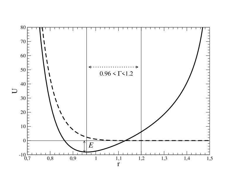
Figure 2: Bounded potential $U_{1}(r)$ (continuous curve) and unbounded potential $U_{2}(r)$ (dashed line) between a pair of monomers. Each monomer can participate to at most two bounded links (with potential $U_{1}(r)$). All unbounded monomer pairs interact via the potential $U_{2}(r)$. E is a parameter tuning the energy required to open the bond. The figure also shows the $\Gamma$ region where potential swaps (equivalent to bond scissions or bond recombinations) are allowed during the brownian dynamics simulation is indicated.

Using the Heaviside function $\Theta(x)=0$ or $1$ for $x<0$ or $x\geq 0$ respectively, explicit expressions (see figure 2) are

$$U_{2}(r) = 4\epsilon\left[(\frac{\sigma}{r})^{12}-(\frac{\sigma}{r})^{6}+\frac{1}{4}\right]\Theta(2^{1/6}\sigma-r))$$ (43)

$$U_{1}(r) = U_{2}(r)-0.5kR^{2}\ln{\left(1-[\frac{r}{R}]^{2}\right)}-U_{min}-E$$ (44)

In the second expression valid for $r<R$, $k=30\epsilon/\sigma^{2}$ is the spring constant and $R=1.5\sigma$ is the value at which the FENE potential diverges. $U_{min}$ is the minimum value of the sum of the two first terms of the second expression (occuring $r_{min}=0.96094\sigma$ for the adopted parameters) while $E$ is a key parameter which corresponds, when pair potential exchanges between bounded and unbounded situations will be allowed, to the typical energy gain (loss) when an unbounded (bounded) pair is the object of a recombination (scission).

We deal with M monomers at temperature $T$ enclosed in a volume V, defining a monomer number concentration $\phi=M/V$. The relevant canonical partition function is a sum over all microscopic states specified not only by monomer positions (and momenta) but also by a set of variables defining unambiguously the connectivity scheme for the particular microscopic state. Disregarding the irrelevant momentum variables in Brownian Dynamics, we write the partition function as

$$Q_{MVT}\sim\sum_{\{r\}}\sum_{m}\exp{(-\frac{U(\{r\},m)}{k_{B}T})}$$ (45)

where the double sum runs over all possible arrangements of M distinguishable monomers and over all related bounding schemes. The first sum runs over all spatial positions $\{r\}$ of the M monomers, each configuration being characterized by a list of K monomer-monomer pairs with relative distance shorter than R. The second sum runs, for a given spatial arrangement with a subset of K pairs available for bounding, over all allowed distinct bounding schemes, namely those among the $2^{K}$ distinct possibilities which satisfy two restricting rules, namely

• no monomer can be engaged into more than two bounding pairs (= no branching).

• no cyclic bounding structure is allowed.

The potential energy associated to a particular configuration can be written

$$U(\{r\},m)=\frac{1}{2}\sum_{i}{\sum_{j\neq i}{(s_{ij}U_{1}(r_{ij})+(1-s_{ij})U_{2}(r_{ij}))}}$$ (46)

where $s_{ij}=0$ for all pairs with $r_{ij}>R$ while $s_{ij}=$ either 0 or 1 for the K pairs with $r_{ij}<R$. Index m in the two previous expressions corresponds to a particular bounding network representing a particular set of 0 and 1 for the K $s_{ij}$ values.

In order to discuss topological changes (change in bounding network) during the phase space exploration, it is useful to consider that each monomer possesses two arms available for bounding. If both arms are free, we have an isolated monomer with degree of polymerisation $L=1$. If at least one arm of a particular monomer is linked through potential $U_{1}(r)$ to an arm of another monomer, these two monomers belong to the same linear structure (micelle) of degree of polymerisation $L\geq 2$. A terminal or an interior monomer will correspond to a monomer engaged respectively in one or two bonds with other monomers.

The phase space exploration will be performed by a Brownian Dynamics (BD) scheme (controling $r$ positions updates) coupled to a single bond creation (replacement of potential $U_{2}(r)$ by $U_{1}(r)$) / single bond annihilation (replacement of potential $U_{1}(r)$ by $U_{2}(r)$) scheme satifying microscopic reversibility.

The BD is standard and samples the set of positions of the M monomers according to a canonical ensemble corresponding to a particular potential energy (equivalent in the present case to a particular bonding network m).

The single BD step of particule i subject to a total force $\overline{F}_{i}$ is simply

$$\overline{r}_{i}(t+\Delta t)=\overline{r}_{i}(t)+\frac{\overline{F}_{i}}{\xi}\Delta t+\overline{R}_{i}(\Delta t)$$ (47)

where the last term corresponds to a vectorial random gaussian quantity with first and second moments given by

$$<{R}_{i\alpha}(\Delta t)> = 0$$ (48)

$$<{R}_{i\alpha}(\Delta t){R}_{j\beta}(\Delta t)> = 2(\frac{k_{B}T}{\xi})\Delta t\delta_{\alpha\beta}\delta_{ij}$$ (49)

for arbitrary particles i and j and where $\alpha\beta$ stand for the $x,y,z$ cartesian components.

At this stage, it is useful to fix units. In the following, we will adopt the size of the monomer $\sigma$ as unit of length, the $\epsilon$ parameter as energy unit and we will adopt $\xi\sigma^{2}/(3\pi\epsilon)$ as time unit. We also introduce the reduced temperature $k_{B}T/\epsilon=T^{*}$, so that in reduced coordinates (written with symbol*) the algorithm becomes

$$<{R}_{i\alpha}^{*}(\Delta t^{*})> = 0$$ (50)

$$<{R}_{i\alpha}^{*}(\Delta t^{*}){R}_{j\beta}^{*}(\Delta t^{*})> = \frac{2}{3\pi}\Delta t^{*}\delta_{\alpha\beta}\delta_{ij}\,T^{*}$$ (51)

which means that each particle, if isolated in the solvent, would diffuse with a RMSD of $\sqrt{2T^{*}/\pi}$ per unit of time.

The bonding network is itself the object of random instantaneous changes provided by a Monte-Carlo algorithm which is built according to the standard Metropolis scheme.

The probability $P_{m,n}$ to go from a bounding network $m$ to a different one $n$ is written as

$$P_{m,n}=A_{m,n}^{trial}P_{m,n}^{acc}$$ (52)

where $A_{m,n}^{trial}$ is the trial probability to reach a new bounding network $n$ starting from the old one $m$, within a single MC step. This trial probability is chosen here to be symmetric as usually adopted in Metropolis Monte Carlo schemes. This trial probability is chosen to be different from zero only if both bounding networks n and m differ by the status of a single bond, say the pair of monomers $(ij)$. To satisfy microreversibilty, the acceptance probability $P_{m,n}^{acc}$ for the trial ($m\longrightarrow n$) must be given by

$$P_{m,n}^{acc}=Min[1,\exp{(-\frac{(U(\{r\},n)-U(\{r\},m))}{k_{B}T})}].$$ (53)

In the present case, as a single pair (ij) changes its status, the acceptance probability takes the explicit form

$$P_{m,n}^{acc} = Min[1,\exp{(-\frac{(U_{2}(r_{ij})-U_{1}(r_{ij}))}{k_{B}T})}]$$ (54)

$$P_{m,n}^{acc} = Min[1,\exp{(-\frac{(U_{1}(r_{ij})-U_{2}(r_{ij}))}{k_{B}T})}]$$ (55)

for bond scission and bond recombination respectively.

The way to specify the trial matrix $A_{m,n}^{trial}$ starts by defining a range of distances, called $\Gamma$ and defined by $0.96<r<1.20$ within the range $r<R$. For $r\in\Gamma$, a change of bounding is allowed as long as the two restricting rules stated above are respected. Consider the particular configuration illustrated by figure 3 where M=7 monomers located at the shown positions, are characterized by a connecting scheme made explicit by representing a bounding potential by a continuous line. The dashed line between monomers 5 and 6 represents the changing pair with distance $r\in\Gamma$ which is a bond $U_{1}(r)$ in configuration $m$ but is just an ordinary intermolecular pair $U_{2}(r)$ in configuration $n$.

For further purposes, we have also indicated in figure 3 by a dotted line all pairs with $r\in\Gamma$ which are potentially able to undergo a change from a non bounded state to a bounded one in the case where the (56) pair, on which we focus, is non bounded (state n). Note that bond (35) is not represented by a dotted line eventhough the distance is within the $\Gamma$ range: a bond formation in that case is not allowed as it would lead to a cyclic conformation. Note also that in state n, monomer 5 could thus form bonds either with monomer 2 or with monomer 6 while monomer 6 can only form a bond with monomer 5.

We now state the algorithm and come back later on the special ($m\longrightarrow n$) transition illustrated in figure 3.

During the BD dynamics, with an attempt frequency $\omega$ per arm and per unit of time, a change of the chosen arm status (bounded $U_{1}(r)$ to unbounded $U_{2}(r)$ or unbounded to bounded) is tried. If it is accepted as a “trial move” of the bounding network, it obviously implies the modification of the status of a paired arm belonging to another monomer situated at a distance $r\in\Gamma$ from the monomer chosen in the first place.

The trial move goes as follows: a particular arm is chosen, say arm 1 of monomer i, and one first checks whether this arm is engaged in a bounding pair or not.

• If the selected arm is bounded to another arm (say arm 2 of monomer j) and the distance between the two monomers lies within the interval $r_{ij}\in\Gamma$, an opening is attempted with a probability $1/(N_{i}+1)$, where the integer $N_{i}$ represents the number of monomers available for bonding with monomer i, besides the monomer j ($N_{i}$ is thus the number of monomers with at least one free arm whose distance to the monomer carrying the originally selected arm i lies within the interval $\Gamma$, excluding from counting the monomer j and any particular arm leading to a ring closure). If the trial change consisting in opening the (ij) pair is refused (either because the distance is not within the $\Gamma$ range or because the opening attempt has failed in the case $N_{i}>0$), the MC step is stopped without bonding network change (This implies that the BD restarts with the (ij) pair being bonded as before).

• If the selected arm (again arm 1 of monomer i) is free from bonding, a search is made to detect all monomers with at least one arm free which lie in the “reactive” distance range $r\in\Gamma$ from the selected monomer i (Note that if monomer i is a terminal monomer of a chain, one needs to eliminate from the list if needed, the other terminal monomer of the same chain in order to avoid cyclic micelles configurations). Among the monomers of this “reactive” neighbour list, one monomer is then selected at random with equal probability to provide an explicit trial bonding attempt between monomer i and the particular monomer chosen from the list. Note that if the list is empty, it means that the trial attempt to create a new bond involving arm 1 of monomer i has failed and no change in the bonding network will take place.

In both cases, if a trial change is proposed, it will be accepted with the probability $P_{m,n}^{acc}$ defined earlier. If the change is accepted, BD will be pursued with the new bonding scheme (state n) while if the trial move is finally rejected, BD restarts with the original bonding scheme corresponfing to state m.

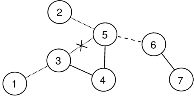
Figure 3: Exemplary configuration of a 7 monomers system in state n where monomers 3,4 and 5 form a trimer and monomers 6 and 7 a dimer. All pairs of monomers with mutual distances within the $\Gamma$ region are indicated by a dotted or a dashed line. In the text, we consider the Monte Carlo scheme for transitions between states n and m which only differ by the fact that in state n and m the 5-6 pair is respectively open or bounded. The n $\rightarrow$ m transition corresponds to the creation of a pentamer by connecting a dimer and a trimer while the m $\rightarrow$ n transition leads to the opposite scission. The cross symbol on link 3-5 indicates that in state n, when looking to all monomers which could form a new link with monomer 5, monomer 3 is excluded because it would lead to a cyclic polymer which is not allowed within the present model.

Coming back to figure 3, we now show that the MC algorithm mentioned above garantees that the matrix $A_{mn}^{trial}$ is symmetric, an important issue as it leads to the micro-reversibility property when combined with the acceptance probabilities described earlier. Let us define as $P_{arm}=1/2N$ the probability to select a particular arm, a uniform quantity.

If configuration m with pair (56) being “bounded” is taken as the starting configuration, the number of available arms to form alternative bonds with monomer 5 and monomer 6 are respectively $N_{5}=1$ and $N_{6}=0$. Therefore, applying the MC rules described above, the probability to get configuration n where the pair (56) has to be unbounded is given by the sum of probabilities to arrive at this situation through selection of the arm of monomer 5 engaged in the bond with monomer 6 or through selection of the arm of monomer 6 engaged in a bond with monomer 5. This gives

$$A_{m,n}^{trial}=P_{arm}*\frac{1}{N_{5}+1}+P_{arm}\frac{1}{N_{6}+1}=\frac{3}{2}*P_{arm}$$ (56)

If configuration n with pair (56) being “unbounded” is taken as the starting configuration, the application of the MC rules lead to the probability to get configuration m where the pair (56) has to be bounded is given by the sum of probabilities to arrive at this situation through selection of the free arm of monomer 5 (which has two bounding possibilities, namely with monomers 2 and 6) or through selection of the free arm of monomer 6 which can only form a bond with monomer 5. This gives

$$A_{n,m}^{trial}=P_{arm}*\frac{1}{2}+P_{arm}=\frac{3}{2}*P_{arm}$$ (57)

showing the required matrix symmetry.

0.5 Characterization of static properties

In the following, all quantities will systematically be expressed in reduced units without an explicit $*$ symbol.

0.5.1 List of experiments and chain length distributions

We consider a system of $M=1000$ monomers interacting via the potential model defined by eqs.(44) at $T=1$. This is a rather small system by nowadays standards but we were only interested here to a preliminary demonstrative study before going in the future to larger systems and a more efficient description of solvent effects.

This system is studied at two state points:

• A dilute solution at the number density $\phi=0.05$ and an energy parameter $E=8$.

• A semi-dilute solution at the number density $\phi=0.15$ and an energy parameter $E=10$.

Each system evolves according to the Brownian Dynamics algorithm with time step $\Delta t=0.001$ and is subject to random trials of bond scission/recombination with arm trial attempts frequencies in the range $0.1<\omega<5$. This choice was motivated by the necessity to speed up the kinetics and hence, getting reasonably good statistics on dynamical properties. Obviously, all static properties are independent of $\omega$ and therefore, all data can be cumulated over all $\omega$ values.

The systems have been equilibrated for a time of $2\ 10^{4}$. Production runs have been followed for a similar time $T_{run}=2\ 10^{4}$. The equilibrium values of the mean chain length $L_{0}$ and the total number of chains $<N_{ch}>$ are related by $M=L_{0}<N_{ch}>$.

The dilute case

The first experiment deals with a dilute solution as the average chain length $L_{0}=10.4\pm 0.1$ is much smaller than the crossover value at that monomer number density as calculated by eq.(21), $L^{*}=50.5$.

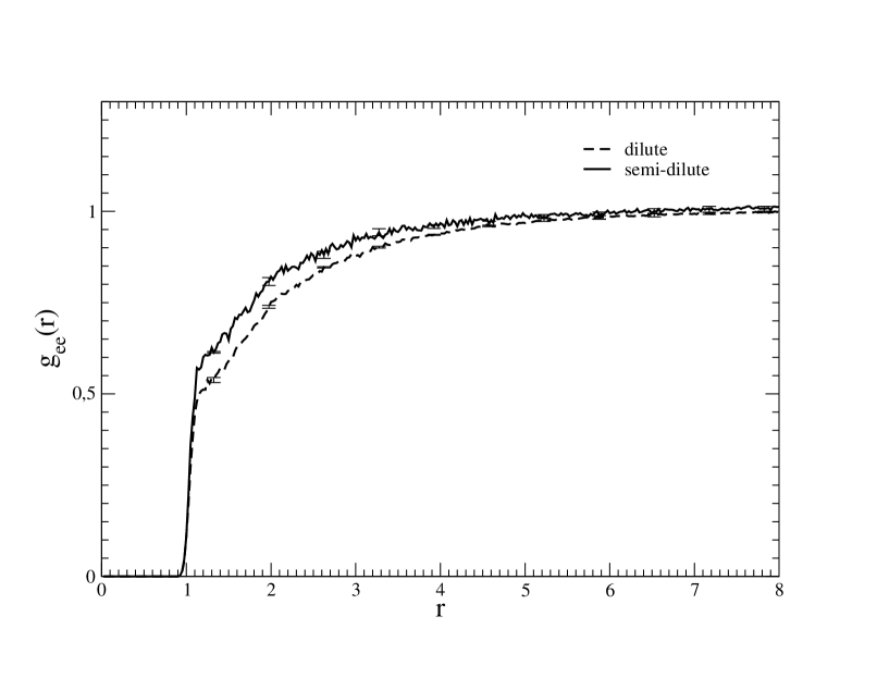
Figure 4: Chain end pair distribution function $g_{ee}(r)$ in the dilute and semi-dilute experiments. Note that the $\Gamma$ region where the bounding changes take place correspond to the region of first (fast) increase of the distribution function around $r=\sigma$.

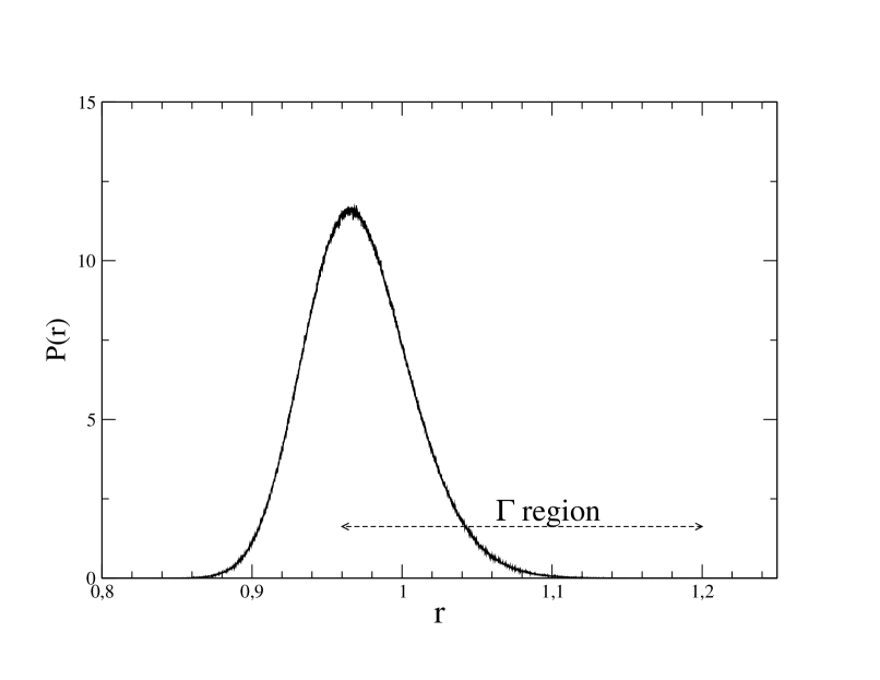
Figure 5: Normalized distribution function $P(r)$ of the distance between bounded monomers in the semi-dilute experiment. The corresponding function in the dilute solution experiment is marginally different from the semi-dilute case and is therefore not shown in the figure.

The populations of bonds ready to open within the $\Gamma$ range is $<N_{1\Gamma}>=551.6$ and represents $61\%$ of the bonded pairs $<N_{1}>$, while the population of free arms pairs ready to close, again within the same $\Gamma$ range, is only $<N_{2\Gamma}>=1.16$. Figures 4 and  5 show respectively the pair correlation function for chain ends (unsaturated arms) and the distribution of the distance between bounded monomers, in particular within the $\Gamma$ region where potential changes do occur. The “free arm” fraction, namely $1-N_{1}/M=0.0957$, is close to $L_{0}^{-1}=<N_{ch}/M>=0.0964$.

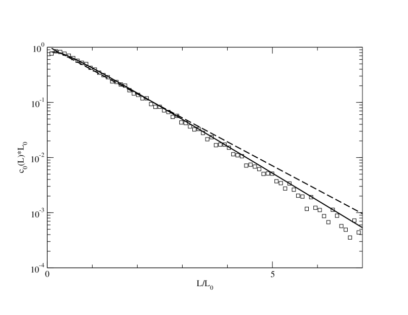
Figure 6: Distribution of chain length number densities for the dilute case in good solvent. The data (squares) are fitted using eq.(30) with imposed value $\gamma=1.165$. The dashed line shows the exponential distribution $C_{0}(L)\propto\exp{(-\frac{L}{L_{0}})}$ which does not fit data as well.

Dilute solution conditions are confirmed by the chain length distribution shown in figure 6. For dilute conditions, a distribution given by eq.(30) is expected. Accordingly, we have fitted our data with a single parameter (prefactor) fit function, $c(L)=A_{0}L^{\gamma-1}\exp{(-\gamma L/L_{0})}$ where $L_{0}$ was given its computed average value and where $\gamma$ was given its expected value, $\gamma=1.165$. This curve is significantly better than the simple exponential distribution expected for ideal or semi dilute chains. If $\gamma$ is left as a second free parameter in the fit, it takes an even larger value $1.187$ and the fit (not shown) is slightly better especially at high L.

The semi-dilute case

In the second state point experiments, the average chain length is found to be $<L>=49.9\pm 0.1$, a value which is much larger than the crossover value $L^{*}\approx 12$ at $\phi=0.15$ according to eq.(20).

The populations of bonds ready to open in the $\Gamma$ region is $<N_{1\Gamma}>=597\pm 1.$, while the population of free arms pairs ready to close is $<N_{2\Gamma}>=0.183$. Distance distributions of unbounded and bounded pairs are given in figures 4 and 5 together with the dilute case data. We note that $g(r)$ function between free ends is not very different between the two cases. The “free arm” fraction $1-N_{1}/M=0.021$ is 5 times smaller than in the dilute case as the chains are 5 times longer.

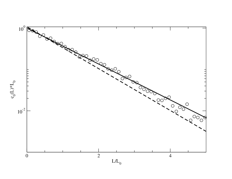
Figure 7: Distribution of chain lengths number densities for the semi-dilute case. The data (circles) are fitted with a simple exponential function $A\exp{(-L/L_{0})}$ (continuous curve), in reference to eq.(34) with imposed average chain size $L_{0}=49.9$. Dashed lines show a function $\exp{(-1.165\frac{L}{L_{0}})}$ which does not fit the data as well.

Semi-dilute solution conditions are confirmed by the observation of an exponential distribution of the reduced chain length (see figure 7). In the latter figure, we show the best fit by a one parameter fitting function $c^{fit}(L)=A\exp{(-L/L_{0})}$.

0.5.2 Chain length conformational analysis

Figures 8 and 9 show for dilute and semi-dilute state points respectively, the average of the square of the radius of gyration and the average of the square of the end-to-end vector as a function of the chain length within the polydisperse sample.

In figure 8 relative to the dilute case, standard power law scaling $L^{2\nu}$ law with $\nu=0.588$ is indicated for long chains. For our polydisperse system with an average chain length of $L_{0}\approx 10$, our data on chains with $L>L_{0}$ are affected by too large statistical error bars to test critically the validity of this asymptotic regime and its exact range of application, limited in the low L regime by usual short chain effects clearly visible below $L=25$.

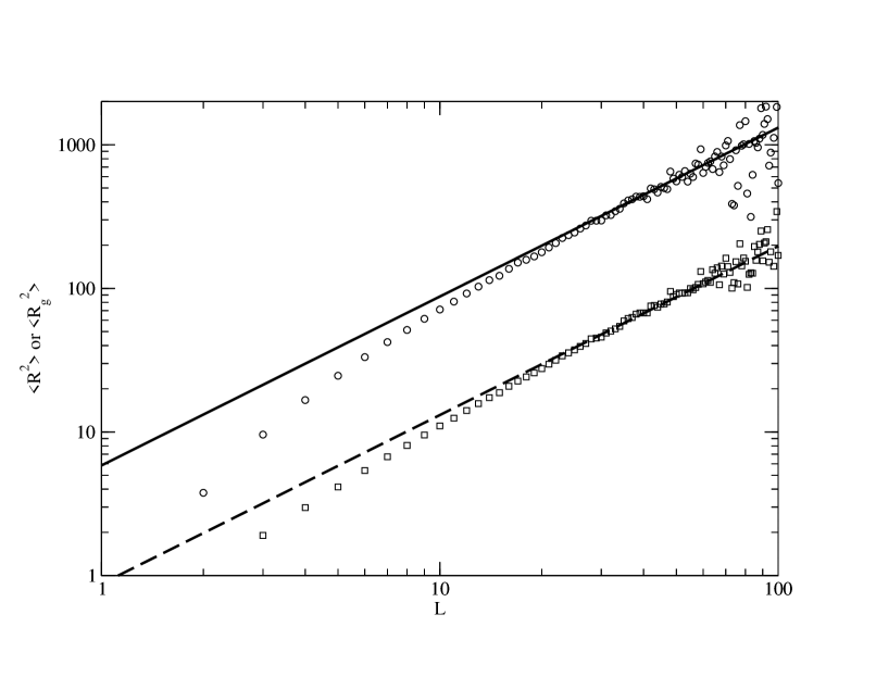
Figure 8: Conformational properties in the dilute case: $<R^{2}>$ (circles) and $<R_{g}^{2}>$ (squares) versus chain length $L$. The fitting functions which are power law with exponent fixed to $2\nu=1.176$ (prefactors $0.876$ for $<R_{g}^{2}>$ and $5.854$ for $<R^{2}>$) fit the data for longer chains only

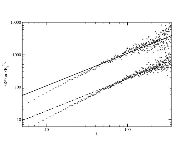
Figure 9: Conformational properties in the semi-dilute case: $<R^{2}>$ (squares) and $<R_{g}^{2}>$ (circles) versus chain length $L$. The fitting functions (linear in L) assume ideal chain statistics with prefactors $1.862$ for $<R_{g}^{2}>$ and $11.06$ for $<R^{2}>$. The fit works for the $L>L^{*}$ behaviour.

The conformational properties of chains in the semi-dilute system are compatible with ideal chains for $L>L^{*}\approx 12$ where $L^{*}$ is estimated from eq.(20) with $\phi=0.15$, and with a larger exponent power law for lower L values but poor statistics and small chain effects prevent a firm test of scaling laws for these semi-dilute chains.

When $<R^{2}>$ data from both state points are plotted versus $L$ on a unique graph (not shown), the short chains behaviours are found to be undistinguishable, while divergences between the two state points are observed for long chains. The power laws shown in figures 8 and 9 intersect at the blob length value of $L^{*}=37$ monomers, giving a blob size or a correlation length of $\chi=<R^{2}>^{1/2}=20$. Note that in this analysis, we implictly assume that the prefactor of the dilute chains power law is independent of $\phi$ while we consider the $\phi$ dependent prefactor in the ideal chain power law corresponding to the semi-dilute state at $\phi=0.15$. We thus see that the blob size as determined from the intersection of asymptotic power laws (neglecting short chains effects) suggest a numerical prefactor of about $3$ in the scaling relations (20). On this basis, our dilute system at $\phi=0.05$ would be characterized by a blob length of $L^{*}=50$ and thus a ratio $L_{0}/L^{*}=0.2$ suggesting a rather clear dilute solution character. The same ratio is $L_{0}/L^{*}=1.4$ for the more concentrated solution showing that the usual concept of chains of blobs in a semi-dilute solution applies only marginally to the longer chains in the sample. To conclude, this analysis indicates that, even in the semi-dilute case, the chain dynamics should not be significantly affected by the weak entanglements between chains. Let us stress that the semi-dilute character of the sample is however well illustrated by static properties such as the exponential chain length distribution and the ideal chain power laws for chain sizes.

0.6 Kinetics analysis

The number of Monte-Carlo “accepted” scissions (or “accepted” recombinations) are obtained by simple counting during the simulations. In table 1 (dilute case) and in table 2 (semi-dilute case), we list the number $n_{s}$ of “accepted” transitions per unit time and unit volume, for the two state points and for the different attempt frequencies $\omega$ investigated. For each state point, we observe that the number of scissions per unit of time is, as expected, proportional to $\omega$ and we have also verified that the number of recombinations differs from the number of scissions by marginal amounts (0.05$\%$), which shows that the chain length distributions are well equilibrated.

Table 1: Kinetic data for the dilute case at four scission-recombination attempt frequencies $\omega$. $n_{s}$ is the total number of Monte-Carlo scissions (recombinations) per unit time and per unit volume. $\alpha$ is the fraction of scissions where newly created free arms recombine with a new partner. Superscript $(i)$ refers to the methodology used to get various estimates of a given quantity, namely $i=1$ for the method based on the distribution of first recombination times, $i=2$ for the cumulative hazard method and $i=3$ for the “reactive flux” approach. $\tau_{b}$ is the average first recombination time and also the typical life time of a chain of average length $L_{0}$. The estimate $\tau_{b}^{(i)}$ is obtained by the long time behaviour of the relevant dynamical function used in methodology (i). $\kappa^{(i)}$ is the fraction of transitions which are effective. Such transitions can be seen as those which do not belong to sequences of correlated transitions (chain scission followed by almost immediate recombination ending into no change in chains topology). An additional estimate of $\tau_{b}$ (not listed in th etable) may be obtained on the basis of $n_{s}$ and $\kappa^{(i)}$ computed with methodology $i$ using $\tau_{b}=\frac{\phi}{L_{0}\kappa^{(i)}n_{s}}$

$\omega$ $\kappa^{(3)}$ $\alpha$ $n_{s}*10^{3}$ $\tau_{b}^{(1)}$ $\tau_{b}^{(2)}$ $\tau_{b}^{(3)}$ 0.1 .89 0.89 (0.80) 0.00759 694. 763. 625. 0.5 0.60 0.68 (0.60) 0.038 196. 212. 185. 1.0 0.45 0.55 (0.48) 0.076 153. 146. 122. 5.0 0.20 0.28 (0.25) 0.38 60.2 67.0 63.3

Table 2: Kinetic data for the semi-dilute case at four scission-recombination attempt frequencies.All quantities are defined in the previous table

$\omega$ $\kappa^{(2)}$ $\kappa^{(3)}$ $\alpha$ $n_{s}*10^{3}$ $\tau_{b}^{(1)}$ $\tau_{b}^{(2)}$ $\tau_{b}^{(3)}$ 0.1 0.85 0.85 0.85 (0.73) 0.0042 919. 885. 813. 0.5 0.52 0.44 0.53 (0.44) 0.022 285. 265. 282. 1.0 0.34 0.35 0.40 (0.31) 0.042 191. 190. 184 5.0 0.12 0.12 0.16 (0.11) 0.21 130. 108. 106.

The quantity $\alpha$ mentioned in the tables is the fraction of scissions which lead to a recombination with a new partner. In our analysis, the fate of a scission has been initially followed for a maximum time of $T_{max}=1000$. The value quoted in parentheses is the ratio obtained by using data for which the recombination time is less than $T_{max}$, while the first value is obtained by assuming that all recombinations taking place beyond that maximum time should be necessarily with new partners, as it is justified by data shown in figure 11 to be discussed later. The product $\alpha n_{s}$ is the number of scissions per unit of time and per unit volume which lead to a recombination with a new partner, that is those which lead to real changes in the distribution of chain lengths.

In the explored $\omega$ range, the value of $\alpha$ indicates that a large fraction of elementary scissions are followed by recombinations of the same original chain fragments. Using $\alpha$ as a measure of the percentage of effective reactions, we observe a decrease of this percentage as the rate of attempted transitions $\omega$ increases. Actually, uneffective transitions may also come from more complex particular transition sequences. Consider a chain end monomer (say monomer $i$) lying close in space to another chain at the level of two adjacent monomers $j$ and $k$. At high $\omega$, a scission of the bond $jk$ may be immediately followed by a recombination between $j$ or $k$ with monomer $i$. In turn, that $ik$ or $ij$ bond may reopen and recombine to restaure the very first situation, ending with no effective transition without being detected through the criterium of a successive recombination with the same partner. The occurence of such events is proven indirectly in the following by noting almost immediate chain end recombination with another partner (see figure 11).

To extract estimates of the rate constants defined by the kinetic model of Cates, it is thus important to eliminate the spurious transitions from the effective ones. The best route for this is certainly to approach the problem via a time scale separation between scission-recombination processes taking place on a fast time scale and effective transitions taking place on the reaction time scale $\tau_{b}$.

0.6.1 Distribution of first recombination times

The first approach is to compute the histogram of first recombination times $t=t_{2}-t_{1}$ for an arm which became free by scission at time $t_{1}$ and which recombined with another free arm at time $t_{2}$. Figure 10 shows the result for the semi-dilute case for the four values of $\omega$. In figure 11 relative to the case $\omega=0.5$ specifically, we show the contribution to the distribution of first recombination times from events implying either the same or a different partner. In the latter figure, one observes that at short time, the recombination with the same partner dominates. However, even at short times, recombinations with another partner are possible as discussed earlier. The two curves corresponding to the two types of contributions cross each other around $t=25$ and at later times, the recombination with another partner progressively dominates. We note however that at times as long as $t=200$ where monomers have diffused by a distance corresponding to three times their size (see figure 9), there is still $10\%$ of recombinations at that time which take place with the same partner.

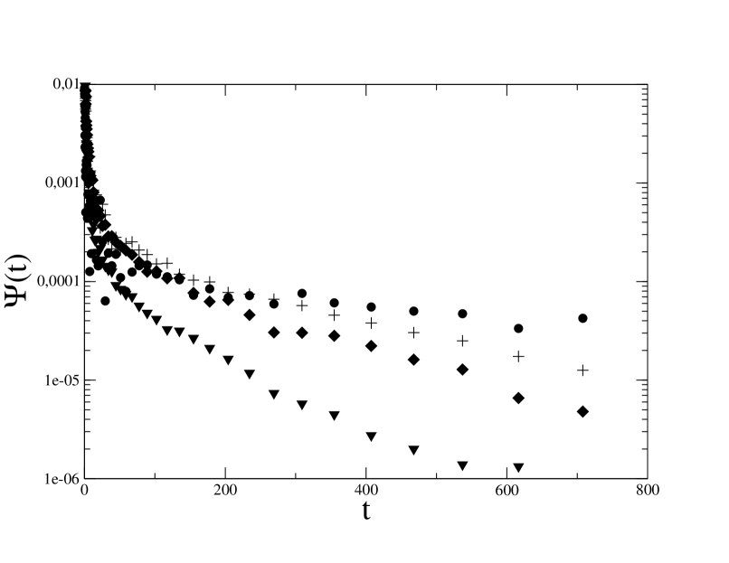
Figure 10: Distribution of first recombination times $\Psi(t)$ for the semi-dilute case. Data are shown for $\omega=0.1$ (filled circles), $\omega=0.5$ ($+$ symbols), $\omega=1.0$ (filled lozenges) and $\omega=5.0$ (filled triangles). Estimates of $\tau_{b}^{(1)}$ are obtained from the slope of a linear fit of $\ln{\Psi(t)}$ versus time in the long time region.

Data of figure 10 have been analyzed by considering that $\Psi(t)$ is exponential at long times. The slope is interpreted as the inverse of the average life time of a chain end which is denoted as $\tau_{b}^{(1)}$. Specific values for the different $\omega$’s are indicated in tables 1 and 2, respectively for dilute and semi-dilute cases.

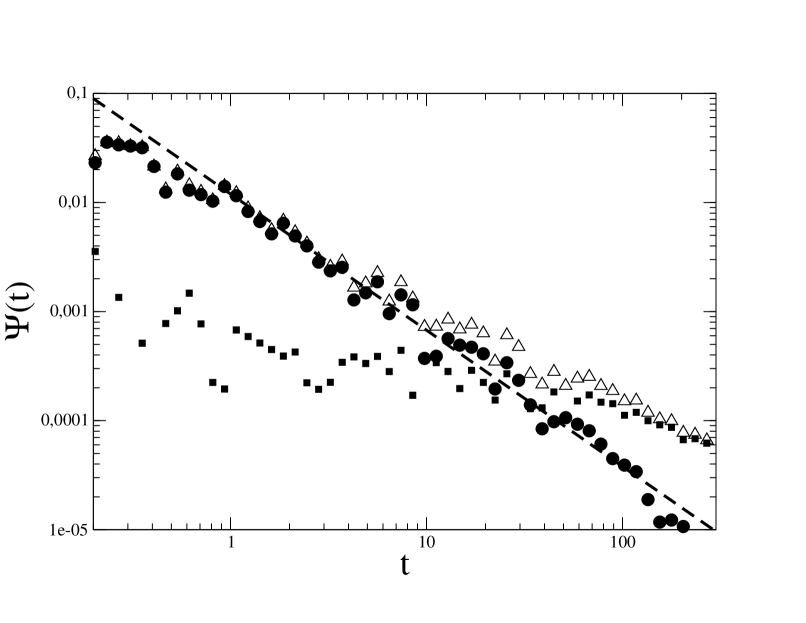
Figure 11: Distribution of first recombination times $\Psi(t)$ for the semi-dilute case for attempt frequencies $\omega=0.5$ (open triangles). The partition between contributions from recombinations with the same partner (filled circles) or with a new partner (filled square) are distiguished. The power law $0.012(t)^{-5/4}$ shows that the “diffusion-controlled” theoretical prediction of $-5/4$ for the power law exponent is perfectly satisfied for the self recombination part for times larger than $t=1$. The picture shows how self-recombinations dominate at short times while recombinations with new partners dominate beyond $t=30$.

The short time behaviour of the distribution can be analyzed by plotting the function versus time on a logarithmic scale. This is done in figure 11 where we distinguish contributions from recombinations with the same partner or with a new partner. The theory of diffusion controlled recombination kineticsoshau predicts an algebraic decay $At^{-5/4}$ for $\Psi(t)$ and we observe that it is perfectly satisfied by our data for the self recombination part for times larger than $t=1$. The picture shows how self-recombinations dominate at short times while recombinations with new partners dominate beyond $t=30$. At very short times (t¡1), a significative part (about $10\%$) of the $\Psi(t)$ function implies recombinations with anorther partner.

0.6.2 Cumulative hazard analysis

To analyse the rates of conformational transitions in butane and other short alkane molecules, Helfand helf suggested to exploit hazard rate plotting. We have adapted this technique to the present case. We first summarize the theoretical foundations of the method, using the particular case of equilibrium polymer kinetics to directly illustrate the concepts.

Let $h(t)dt$ be the probability that a free arm, created at time $t=0$ and which is still free at time t, undergoes a first recombination in the interval $[t,t+dt]$. Let $P(t)$ be the probability that a free arm, created at time $t=0$, has undergone a (first) recombination between 0 and t.

Using these definitions, the following steps can be written

$$\left[1-P(t+dt)\right] = \left[1-P(t)\right](1-h(t)dt)$$ (58)

$$\frac{d}{dt}\left[1-P(t)\right] = -h(t)\left[1-P(t)\right]$$ (59)

$$\left[1-P(t)\right] = \exp{(-\int_{0}^{t}h(t^{\prime})dt^{\prime})}=\exp{\left[-H(t)\right]}$$ (60)

where $H(t)=\int_{0}^{t}h(t^{\prime})dt^{\prime}$ is the cumulative hazard. In the present case, we anticipate a complex process involving correlated events at short times $h(t)=h^{sh}(t)$ and a Poisson process emerging at long times with uniform frequency $lim_{t\rightarrow\infty}h(t)=\lambda$ where $\lambda$ is the recombination rate constant. On the relevant time scale of the kinetics, one thus should find for the cumulative hazard function and the P(t) probability

$$H(t) = H_{I}+\lambda t$$ (61)

$$P(t) = 1-\exp{(-H_{I})}\exp{(-\lambda t)}$$ (62)

where $H_{I}$, the ordinate intercept of the function $H(t)$ versus t, can be seen as the time integral of $(h^{sh}(t)-\lambda)$ from $0$ to $\infty$. If a good time scale separation exists, eq.(62) implies that $c\equiv P(0^{+})=1-\exp{(-H_{I})}$ is the fraction of correlated transitions, $\kappa^{(2)}=1-c$ being the estimate according to the present analysis of the average probability for a newly created free arm to recombine by the Poisson “mean field” kinetic process postulated by Cates in his theorycates .

We now explain how the estimate of the cumulative hazard function is constructed. We start by extracting from the BD trajectory a collection of times $\{\hat{t}\}$ where each member corresponds to the elapsed time between a scission of a particular arm at time $t_{1}$ and its next recombination at time $t_{2}$, so $\hat{t}=t_{2}-t_{1}$. All the $2M$ arms of the system contribute to the $\hat{t}$ data sample which, for each arm, can contain several times of this kind between the start (at $t=0$) and the end (at $t=T_{max}$) of the BD trajectory.

Moreover, if the first change of status of a particular arm since the beginning of the BD simulation is a recombination taking place at time t, we can say that this time is a lower bound $\hat{T}$ of an additional unknown elapsed time $\hat{t}$ between a scission (out of our reach) and the next recombination (we observed). Also, if the last change of arm status before the end of the BD trajectory is a scission taking place at time t, then, the time $\hat{T}=T_{max}-t$ is a similar lower bound of yet another time of interest. The analysis thus furnishes a set of $K$ times $\{\hat{t}\}$ and $M$ lower bounds times $\{\hat{T}\})$ which are then separately ordered from the shortest time up to the longer one and indexed accordingly as $(\hat{t}_{1},\hat{t}_{2},\hat{t}_{3},..\hat{t}_{K})$ and $(\hat{T}_{1},\hat{T}_{2},\hat{T}_{3},...\hat{T}_{M})$. Let us consider successively all individual arm life times $\{\hat{t}\}$. For any time $\hat{t}_{i}$ of that collection, the probability that a free arm which had survived up to the previous time $\hat{t}_{i-1}$ changes its status and becomes engaged in the formation of new bond between times $\hat{t}_{i-1}$ and $\hat{t}_{i}$ is given with our available statistics by $1/N(\hat{t}_{i-1})$ where the denominator is the number of cases (including both types of times $\hat{t}$ and $\hat{T}$) where recombination takes place at a time longer than $\hat{t}_{i-1}$, i.e.

$$N(\hat{t}_{i-1})=[K-(i-1)]+[M-m_{(i-1)}]$$ (63)

where $m_{(i-1)}$ is the index of largest $\hat{T}$ value which is still inferior to $\hat{t}_{i-1}$. In terms of these definitions, the cumulative hazard function $H(t)$ can be evaluated at each time $\hat{t}$

$$H(\hat{t}_{i})=\sum_{j=1}^{i-1}\frac{1}{N(t_{j})}$$ (64)

If the function is linear in time, it implies a Poisson process with a rate of transitions given by the slope of that linear portion.

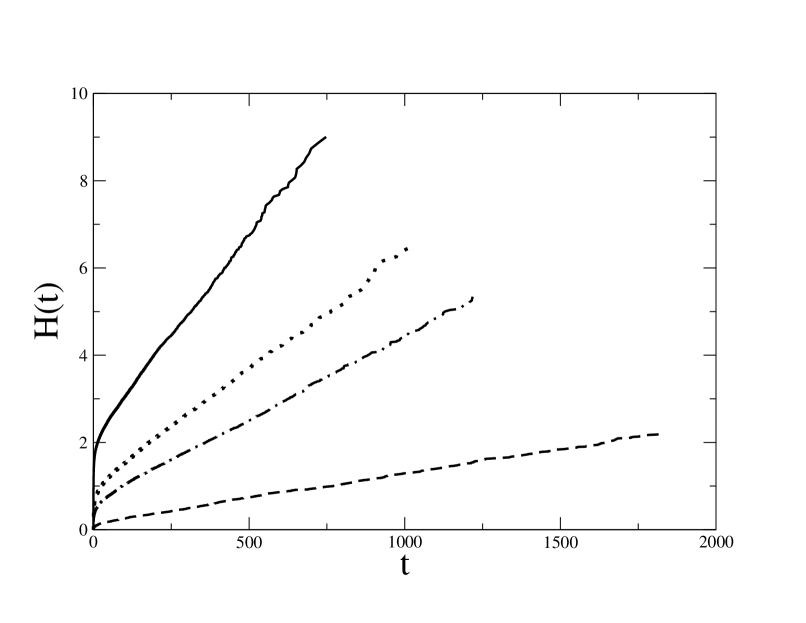
Figure 12: Cumulative Hazard curves of recombination times for the semi-dilute case. Data are shown for various attempt frequencies, namely $\omega=0.1$ (dashed line), $\omega=0.5$ (dot-dashed line), $\omega=1.0$ (dotted line) and $\omega=5.0$ (continuous line).

Figure 12 shows the resulting cumulative hazard functions for the four $\omega$ values in the semi-dilute case. A linear behaviour starts around $100-150$ in all cases and it lasts up to times of the order of $1000$ where statistical noise sets in. The inverse slopes of the linear portions provide estimates $\tau_{b}^{(2)}$ of the mean life time of a chain end. Specific values for both thermodynamic states are gathered in table 1 and table 2. They are compatible with the values extracted from the histogram of first recombination times. Using the procedure described at the beginning of this section, one gets from the ordinate intercepts of $H(t)$ the $\kappa^{(2)}$ estimate indicated in table 2 for the semi dilute case.

The cumulative hazard plot has the advantage that it avoids the necessity of bining recombination time data which become scarse at long times. It also exploits statistically some additional information (useful for low rates) from portions of the $2M$ trajectories between a scission and the next recombination in a way which is truncated either at the beginning or at the end of the BD run.

0.6.3 The reactive flux correlation function and the transmission coefficient

We now discuss still another way to isolate short time transitional effects in order to estimate the rate of “effective” transtions. It relies on the way so-called “Transition State Theory” (TST) values of chemical reactions rates can be corrected by a multiplicative transmission coefficient $0<\kappa<1$ which takes into account the fraction of events where the products formed by the forward reaction are effective transitions. By effective, it means that after such a transition, the product is able to relax its energy excess (which was accumulated to cross the forward barrier) sufficiently quickly to avoid an immediate recrossing of the barrier in the backward direction.

In our case, the analogy is clear. If a bond scission is followed by the same bond recombination within a short microscopic time scale (too short for relative diffusion to take place), it basically means that no effective scission has happened to the chain to which the bond belongs on time scales larger than the relaxation time of a chain fragment of a few monomers.

We have thus estimated $\kappa^{(3)}$ by exploiting the concept of the reactive flux correlation function, as explained by Chandler in the framework of an equilibrium between forward and backward unimolecular reactionschand . We assume here that for an equilibrium between forward unimolecular reactions (chain breaking) and bimolecular backward reactions (end-chain recombinations), the same conceptual expression can still be applied for the forward reaction.

Let us consider one specific arm (among the two of one particular monomer) which is labelled by an index $i$ and to each arm, we associate a signature variable $S_{i}(t)$ which is equal to unity if the ith arm is free at time $t$ and equal to zero if the arm is engaged in a binding with another monomer at that time. Crossings are then characterized by a step change of the $S_{i}(t)$ values, $S_{i}(t)$ going from 0 to 1 or from 1 to 0 for scissions and recombinations respectively. A statistics over all crossing events is defined: for each individual crossing, we set the time at crossing to zero, denoting times very shortly after or before the transition by $t=0^{+}$ and $t=0^{-}$. The reactive flux correlation function is then defined bybrown

$$C_{RF}(t)=2<\left[S_{i}(0^{+})-S_{i}(0^{-})\right]S_{i}(t)>_{cross}$$ (65)

where the average is performed over all crossings (both scissions and recombinations). If we treat separately the averages on scissions and recombinations, we get the equivalent alternative formulation

$$C_{RF}(t)=<S_{i}(t)>_{scissions}-<S_{i}(t)>_{recombinations}$$ (66)

This function starts from unity at very short (positive) times with the first term being one and the second being zero. On very long times (long respect to the relevant inverse kinetic rate constants), this function goes to zero as it is the difference of two averages which ultimately converge to the same equilibrium average value $<S_{i}>$.

Figure 13: Reactive flux correlation function in the semi-dilute case for $\omega=0.5$. The dashed line corresponds to a fit by a function $\kappa\exp{(-t/\tau_{b})}$ in the time region $150<t<500$. Best parameters found are $\kappa^{(3)}=0.48$ and $\tau_{b}^{(3)}=282$.

If all transitions are effective, the reactive flux function will decrease smoothly from 1 to zero reflecting only the kinetics of these effective recombination and scissions. If transitions are often followed by opposite transitions within a short time scale $\tau_{micro}$ or if successive transitions are correlated within such a short time, this will be reflected in the reactive flux by a fast initial decay over that microscopic time. At later times, the macrocopic kinetics (the one considerd by mean field theoretical expresions) will be reflected by the $C_{RF}(t)$ evolution towards zero on a macroscopic time scale, $\tau_{macro}$. The transmission coefficient $\kappa^{(3)}$ is thus estimated as the initial value of the “slow” decay part of that $C_{RF}(t)$ function. This can be expressed as

$$\kappa^{(3)}=C_{RF}(\tau_{micro})$$ (67)

with the requirement of a good time scale separation, that is $\tau_{micro}\ll\tau_{macro}$.

Figure 13 shows the $\omega=0.5$ case for the semi-dilute case already discussed in fig 11 in the context of the distribution of first recombination after a scission. This curve is more difficult to analyse because it is difficult on the basis of this sole function to decide when the behaviour of $ln(C_{RF}(t))$ really becomes close from a linear behaviour. We had to rely on our experience with the distribution $\Psi(t)$ and the cumulative hazard function $H(t)$ for that state point and $\omega$ value. As both functions suggest that the simple “mean field” process emerges at times later than 150, we have fitted the $C_{RF}(t)$ data by an exponential function $C_{RF}^{fit}(t)=\kappa^{(3)}*\exp{(-t/\tau_{b}^{(3)}})$ in the accessible time window above $t=150$. In the present case, we see that there is no real time scale separation between a short time behaviour, observed in the $0<t<150$ regime, and the macroscopic time scale $\tau_{b}^{(3)}$ which is equal to $\approx 280$. Nevertheless, the value of $\tau_{b}^{(3)}$ turns out to be rather close to the other estimates of a chain end average life time and the $\kappa^{(3)}$ value will be shown in the next subsection to lead to a reasonable correction of $n_{s}$, the total number of transitions per unit of time and unit volume quoted in tables 1 and 2. Results of $\kappa^{(3)}$ and $\tau_{b}^{(3)}$ for all $\omega$’s and both state points are included in the tables 1 and 2.

0.6.4 Estimation of rate constants: comparison of the various methods

Explicitly, the scission rate constants $k_{s}$ and $k_{r}$ of the “mean-field” kinetic model can be estimated from our data in two distinct ways.

• On the basis of the total number of transitions $n_{s}$ per unit time and per unit volume, and on the basis of an estimate of $\kappa$ by one of the methods discussed above, the rates can be estimated from a trivial modification of eqs.(40,41), namely

  $$\kappa n_{s}=k_{s}\phi=\frac{k_{r}\phi^{2}}{2L_{0}^{2}}$$ (68)

• On the basis of the long time behaviour of a dynamical function relevant to the particular methodology adopted, the “chain end” life time can be directly estimated. As the latter is equivalent to the typical life time of a chain of average length denoted as $\tau_{b}$, one gets rate constants through the equivalence

  $$\tau_{b}=\frac{1}{k_{s}L_{0}}=\frac{2L_{0}}{k_{r}\phi}$$ (69)

  where the last equality follows from detailed balance requirements.

Tables 1 and 2 provide all needed data. We find that the implicit time scale separation inherent to all analyses provide compatible estimates of the effective rate constants. This can be verified by applying eqs (68) and (69) with the particular estimate of the left hand side.

Looking at all values in the tables, we get an overall consistency between all methodologies. It indicates that all our strategies to extract the “macroscopic” rate constants do work. Among them, the cumulative hazard analysis appears the most straightforward to analyse once $H(t)$ is known and particularly robust as noise influence seems minimal.

We are now in a position to compare the percentage of effective transitions $\kappa$ based on a time scale separation and the $\alpha$ value based on the percentage of recombinations involving a new partner respect to the one left by scission. We observe in the two tables that both estimates are reasonably consistent and quickly decrease for $\omega$ increasing. Fine analysis suggests however that some distinction exists between both quantities in the present case, that is a free Rouse relaxation type of dynamics in solution for moderately long chains. It requires further analysis and the consideration of more entangled cases to make progress on that point. Finally, it should be stressed that while diffusion controlled and mean field kinetics have sometimes been opposed to each otherpadd , it appears in our analysis that they consistently describe short time correlation effects dominated by self recombinations and long time kinetics dominated by recombinations with new partners.

0.6.5 Analysis of the monomer diffusion

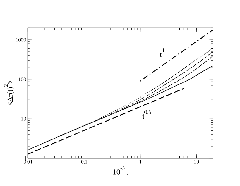
Figure 14: Mean square displacement of monomers (semi-dilute case). The continuous curve has been obtained for the relevant polydisperse sample but with $\omega$ set to zero, averaging over many independent initial configurations. It is a reference from which the other curves depart at decreasing times when increasing values of $\omega$ are considered. The cases $\omega=0.1$ (dashed lines), $\omega=0.5$ (dot-dashed lines) and $\omega=5.0$ (dotted lines) are shown together with two indicative power laws which suggest the evolution of the subdiffusive scaling regime to the normal diffusion limit.

The mean squared displacement (MSD) of all monomers as a function of time is shown in Figure 14 for all $\omega$’s in the semi-dilute case. As these monomers belong to a polydisperse set of chains which continuously break and recombine, the interpretation of the MSD is rather complex.

• Being a single monomer property, a relevant quantity is the average fraction of monomers belonging to chains of length L, namely a distribution $\propto L*c_{0}(L)$. Fig 15 shows the resulting curve for the adopted semi-dilute conditions with $<L>=49.9$.

• The time scale for the scission/recombination process has been estimated so far in terms of the average survival time $1/(k_{s}<L>)$ for the polymer of average size, a quantity which was found to vary from $\approx 100$ up to $\approx 900$ in the investigated $\omega$ range (see table 2). In the present context, we need to consider the explicit L dependent average survival time $\propto 1/(k_{s}L)$ for a given $\omega$ value and figure 15 shows the resulting functions for two such frequencies.

• To discuss the monomer mean squared displacement, it is also important to have an estimate of the longest internal relaxation (Rouse) time of the chains. Performing a separate brownian dynamics run on a monodisperse sample of 20 “dead” polymers of length L=50 (corresponding to the mean polymer length of our living polymer sample) at the same semi-dilute state point ($T=1$, $\phi=0.15$), we get from the long time exponential bevaviour of the end-to-end vector relaxation function a value of $\tau_{R}=4.24\ 10^{3}$. For our very flexible polymers, the scaling of the Rouse time with L in the semi-dilute conditions should scale as

  $$\tau_{R}(L)=AL^{2}.$$ (70)

  On the basis of our estimated value for $L=50$ chains, we get $A\approx 1.70$, a value which can be compared (at least its order of magnitude) to theoretical estimate gennes ; roumil $A\approx\tau_{blob}/(L^{*})^{2}$ in terms of $\tau_{blob}$, the blob relaxation time, and $L^{*}$, the number of monomers per blob. We get $A=5.8$ for our conditions (see discussion in the section on chain conformational properties) where the number of monomers per blob $L^{*}\approx 37$ and $\tau_{blob}\approx\frac{\eta_{s}\chi^{3}}{T}\approx 8000$ using a blob size $\chi=20$ and a solvent viscosity $\eta_{s}=\frac{\xi}{3\pi\sigma}=1$ estimated from the friction coefficient using the Stokes law with an hydrodynamic radius fixed to $\sigma/2$.

On the basis of the above considerations, it is useful to define a particular chain length $\Lambda$ for which the Rouse time is equal to the survival time, giving $\Lambda=(1.7*k_{s})^{-1/3}$, that is $\Lambda=30,20,18,15$ for $\omega=0.1,0.5,1.0,5.0$ respectively. Chains longer than $\Lambda$ have their internal dynamics strongly altered by scissions, while chains shorter than $\Lambda$ should have an internal dynamics little affected with respect to dead polymers of the same size. As figure 15 illustrates, when the scission attempt frequency increases, the fraction of monomers which belong to chains whose dynamics is little affected by scissions decreases.

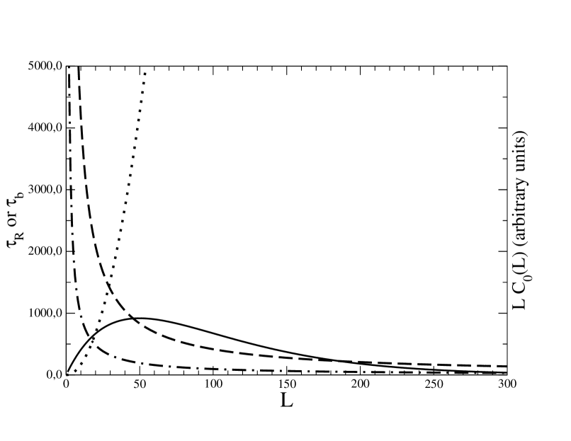
Figure 15: Characteristic times as a function of polymer size. The Rouse relaxation time $\tau_{R}=1.70*L^{2}$, shown as dotted curve, must be compared to the life time of a polymer of size $L$, as given $\tau_{b}=(k_{s}L)^{-1}$. Two frequencies are illustrated, namely $\omega=1.0$ (dot-dashed line) and $\omega=0.1$ (dashed line) using effective $k_{s}$ values. We show on the same graph the distribution of monomers (continuous curve) as a function of the size of the polymer they belong to (see text).

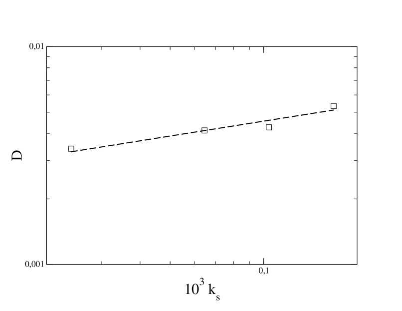
Figure 16: Monomeric Einstein diffusion coefficient as a function of $k_{s}$ for the semi-dilute case. The value of $D$ was obtained from the long time behaviour (beyond t=8000) of the monomeric mean square displacement shown in figure 14. The dashed line represent a $k_{s}^{0.23}$ power law.

Up to a time of 100, the MSD shown in figure 14 is $\omega$ independent and presents a Rouse like behaviour with a time scaling exponent $t^{0.6}$. In the reference case where $\omega$ was set to zero (we simulate polydisperse sample of dead polymers), this power law bahaviour persists at least up to time 10000, a time corresponding to the Rouse time of a chain of length $170$. When scissions and recombinations are allowed, the MDS deviates from the master curve (of dead polymers) to adopt progressively a MSD linear in time. This takes place sooner and sooner for increasing values of $\omega$. At long times ($t>2000$), the MSD has evolved towards usual Einstein diffusion with a diffusion coefficient increasing with $k_{s}$. In figure 16, D is observed to (very roughly) scale like $k_{s}^{0.23}$ in the explored range, a result which is not so far from the $1/3$ power behaviour observed by Milchev with the lattice BFM lattice milch , but which requires further analysis with better estimates of $D$ as statistics is poor above t=10000. The $1/3$ power law scaling is explained by assuming that clusters of $\Lambda$ monomers are responsible of the long time behaviour of living polymers, giving $D\propto\frac{R_{g}^{2}(\Lambda)}{\tau_{Rouse}(\Lambda)}\propto\Lambda^{-1}\propto k_{s}^{1/3}$.

0.6.6 Analysis of the first recombination times distribution and corresponding diffusive steps

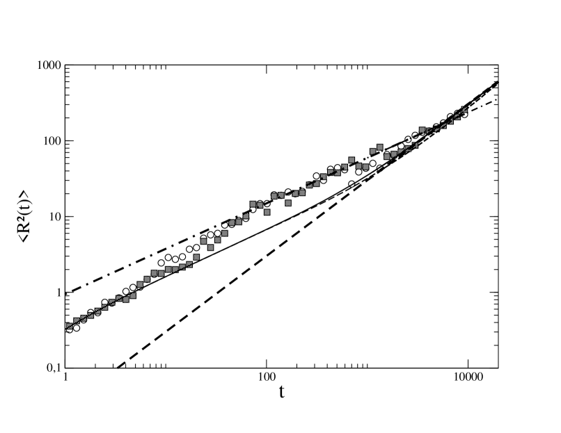
Figure 17: Mean square displacement of end chain monomers between a time set to zero when produced by scission up to a time $t$ corresponding to their first recombination, as a function of their total life time $t$. Due to poor statistics,only data for $\omega=1$ (filled squares) and $\omega=5$ (empty circles) are shown and are limited to $t=10000$ maximum. Data on the mean square displacement of all monomers for corresponding $\omega$ values already shown in figure 14 are shown again here for comparison (see text) up to a maximum time of 20000. Scaling power laws $1.0t^{1.0}$ (thick dashed line) and $0.943t^{0.6}$ (thick dot-dashed line) shown up to t=20000 are used in the text.

In figure 17, we report for two different bond change attempt frequencies $\omega$, the mean squared displacement of a chain end between its creation and its next recombination, as a function of the corresponding life time of that chain end. Interestingly, we observe a common behaviour of this dependence for both frequencies, meaning that the diffusive dynamics of chain ends is little sensitive to the scission/recombination processes of the chains as a whole.

As chain ends have very different life times for different $\omega$’s, the typical average distance travelled by a chain end between its creation and its recombination is also function of that frequency. Mean travel distances of 3.8, 4.6 and 6.8 are obtained for the average chain end life times at $\omega=$5.0, 1.0 and 0.1 respectively, to be compared with the mean static distance between chain ends (assuming no spatial correlations) given by $h=(<L>/2\phi)^{\frac{1}{3}}$ which turns to be $h=5.5$ in our semi-dilute case. By comparison, the radius of gyration of the average chain length in the system is $R_{g}(<L>)\approx 10$. The dynamic picture is thus that chain ends diffuse similarly with time in an environment of other chains which continuously break and recombine. As the reacting frequency increases, the probability of a chain end to recombine with a neighbouring monomer increases and thus takes place earlier, after diffusion over a shorter distance.

0.7 Summary and conclusions

In this paper, we have proposed a new version of a mesoscopic model of equilibrium polymers in solution and we have exploited this model to study the structure and the dynamics of these complex systems at a dilute and at a semi-dilute state point.

The dynamics at the semi-dilute state point has been more specifically investigated. Our system consists of chains with an average number of $L_{0}\approx 50$ monomers which can be viewed as a collection of blobs of $\approx 37$ monomers. Given the large flexibility of the model and the moderately semi-dilute character, our polydisperse polymer solution should be in a non-entangled dynamic regime, with a chain relaxation time growing with chain length L as $L^{2}$.

Working with a unique chain length distribution governed by the structural and thermodynamic microscopic parameters, we have analyzed the specific influence of the Monte Carlo binding/unbinding change attempt frequency on the dynamical properties. Mean field theories are found to be valid for times of the order and beyond the mean life time of a chain of average size provided the kinetic constants computed from the Monte Carlo accepted binding/unbinding changes are rescaled by a transmission coefficient which is a measure of the fraction of successful scissions. This transmission coefficient, when estimated on the basis of a time scale separation, turns out to be close to the fraction of recombinations involving the reunion of a chain end with a new partner and no longer with the monomer it was attached to previously.

The rate constants have been estimated by different techniques which give coherent estimates. The cumulative hazard function introduced by Helfand to compute isomerisation rates in chain molecules has been found to be particularly efficient and simple to implement. In paticular, we find agreement between 1) kinetic constant estimates based on the the total number of transitions rescaled by the transmission coefficient coming from a diffusion controlled mechanism and 2) estimates based directly on the time scale of the long time exponential decay of relaxation functions (mean field Poisson process). It would be interesting to perform so-called T-jump experimentsroumil with our system to test whether the time evolution of the average polymer length $L_{0}$ towards its new equilibrium value at a different temperature confirms the mean field analytical prediction with the kinetic constants computed in the present work from various population relaxation functions at equilibrium.

The chain size that we chose originally was adequate to demonstrate the validity of the methodological aspects developped in this work. In order to test dynamical scaling with a wider range of the scission-recombination process frequency, longer chains will be needed which may require better optimized methods to take solvent effects into account. The extension of this study towards the rheological properties of our model system are under way.

References

- (1) P. van der Schoot, in “Supramolecular polymers” Ed. A. Ciferri, 77 (N.Y. 2005)
- (2) M.E. Cates and S.J. Candau, J. Phys: Cond. Matt. 2, 6869(1990)
- (3) S. Lerouge, J.P. Decruppe and C. Humbert Phys. Rev. Lett. 81, 5457(1998)
- (4) H. Hoffmann, S. Hoffmann, A. Rauscher and J. Kalus, Prog. Colloid Polym. Sci. 84, 24(1991)
- (5) A. Ott, J.P. Bouchaud, D. Langevin, W. Urbach, Phys. Rev. Lett., 65, 2201 (1990).
- (6) P.G. de Gennes, Scaling concepts in polymer physics Cornell University Press, Ithaca(1979)
- (7) A.Y. Grosberg and A.R. Khokhlov, Statistical Physics of Macromolecules AIP Press, New-York(1994)
- (8) M. Doi and S.F. Edwards, The theory of polymer dynamics Clarendon, Oxford(1986)
- (9) M.E. Cates, Macromolecules 20, 2289(1987)
- (10) N.A. Spenley, M.E. Cates and T.C.B. MacLeish Phys. Rev. Lett. 71, 939(1993)
- (11) S.M. Fielding and P.D. Olmsted Phys. Rev. Lett. 90, 224501(2003)
- (12) B. O’Shaughnessy and J. Yu, Phys. Rev. Lett. 74, 4329(1995)
- (13) J.P. Wittmer, A. Milchev and M.E. Cates Europhys. Lett. 41, 291(1998); J. Chem. Phys. 109, 834(1998)
- (14) A. Milchev, in “Computational methods in colloid and interface science” Ed. M. Borowko and M. Dekker, 510(N.Y. 2000)
- (15) Y. Rouault J. Chem. Phys. 111, 9859(1999)
- (16) J.T. Padding and E.S. Boek, Europhys. Lett. 66, 756(2004)
- (17) M. Kroger and R. Makhloufi Phys. Rev. E 53, 2531(1996)
- (18) C.C. Huang, H. Xu and J.P. Ryckaert, manuscript in preparation,(2005)
- (19) D. Chandler, Introduction to Modern Statistical Mechanics , Oxford University Press (1987)
- (20) K. Kremer and G.S. Grest, J. Chem. Phys. 92, 5057(1990)
- (21) A. Milchev, J.P. Wittmer, and D.P. Landau Monte Carlo Study of Equilibrium Polymers in a Shear Flow EPJ B, 12, 2, pp. 241-251 (1999); cond-mat/9905336.
- (22) A. Milchev, J.P. Wittmer, P. van der Schoot, D. Landau Europhysics Letters, 54 58-64 (2001); conf-mat/0008276.
- (23) J.P. Wittmer, M.Milchev, P. van der Schoot, J.-L. Barrat J. Chem. Phys., 113 (2000) 6992-7005; cond-mat/0006465.
- (24) E. Helfand, J. Chem. Phys. 69, 1010(1978)
- (25) D. Brown and J.H.R. Clarke, J. Chem. Phys. 93, 4117(1990)
- (26) Y. Rouault and A. Milchev, Eur. Phys. Lett. 33, 341(1996)