Quantum Dots: Coulomb Blockade,
Mesoscopic Fluctuations, and Qubit Decoherence

Abstract

Quantum Dots: Coulomb Blockade,
Mesoscopic Fluctuations, and Qubit Decoherence

The continuous minituarization of integrated circuits is going to affect the underlying physics of the future computers. This new physics first came into play as the effect of Coulomb blockade in electron transport through small conducting islands. Then, as the size of the island $L$ continued to shrink further, the quantum phase coherence length became larger than $L$ leading to mesoscopic fluctuations – fluctuations of the island’s quantum mechanical properties upon small external perturbations. Quantum coherence of the mesoscopic systems is essential for building reliable quantum computer. Unfortunately, one can not completely isolate the system from the environment and its coupling to the environment inevitably leads to the loss of coherence or decoherence. All these effects are to be thoroughly investigated as the potential of the future applications is enormous.

In this thesis I find an analytic expression for the conductance of a single electron transistor in the regime when temperature, level spacing, and charging energy of an island are all of the same order. I also study the correction to the spacing between Coulomb blockade peaks due to finite dot-lead tunnel couplings. I find analytic expressions for both correction to the spacing averaged over mesoscopic fluctuations and the rms of the correction fluctuations.

In the second part of the thesis I discuss the feasibility of quantum dot based spin- and charge-qubits. Firstly, I study the effect of mesoscopic fluctuations on the magnitude of errors that can occur in exchange operations on quantum dot spin-qubits. Mid-size double quantum dots, with an odd number of electrons in the range of a few tens in each dot, are investigated through the constant interaction model using realistic parameters. It is found that the number of independent parameters per dot that one should tune depends on the configuration and ranges from one to four. Then, I study decoherence of a quantum dot charge qubit due to coupling to piezoelectric acoustic phonons in the Born-Markov approximation. After including appropriate form factors, I find that phonon decoherence rates are one to two orders of magnitude weaker than was previously predicted. My results suggest that mechanisms other than phonon decoherence play a more significant role in current experimental setups.

2005

To my grandmother Vorozhtsova, Tatyana Ivanovna (1917-1987)

Chapter 0 Introduction to Quantum Dot Physics

1 Overview

Quantum dot research [1, 2, 3, 4] has developed into an exciting branch of mesoscopic physics. Many novel phenomena were observed in transport measurements through quantum dots: Coulomb blockade [5], even-odd asymmetry in Coulomb blockade peak spacings [6, 7], and Kondo effect [8, 9] to name just a few. The field has kept researchers busy for about twenty years now and still continues to surprise us.

By no means can I provide a detailed introduction to the entire field in this thesis (even restricting myself to quantum dot physics alone) and I do not think it is necessary as there are quite a few nice review papers available [5, 10, 11, 12]. Instead, I give just enough introductory material on 2D lateral and 3D quantum dots so that the reader can jump into the chapters where the original results of my research are presented.

2 2D Lateral Quantum Dots

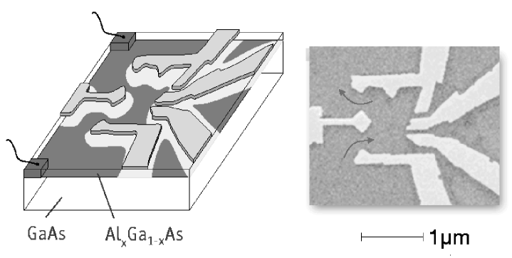
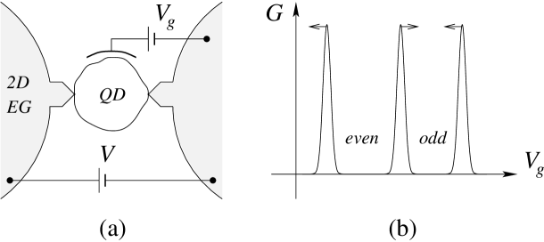
Recent advances in materials science made possible the fabrication of small conducting devices known as quantum dots. In particular, in 2D lateral quantum dots from one to several thousand electrons are confined to a spatial region whose linear size is from about 40 nm to 1$\,\mu$m [2, 13]. These quantum dots are typically made by (i) forming a two-dimensional electron gas on the interface of semiconductor heterostructure and (ii) applying electrostatic potential to the metal surface electrodes to further confine the electrons to a small region (quantum dot) in the interface plane [4], see Fig. 1.

Figure 1: 2D lateral quantum dot. Left panel: Schematic picture of the quantum dot setup. Two-dimensional electron gas is formed on the the AlGaAs/GaAs heterostructure interface. Metal electrodes (or gates) are deposited on top of the heterostructure. Negative voltages are applied to the electrodes to repel the electron gas underneath – bright regions contain no electrons. Then, bias voltage is applied between source and drain leads (see wires coming out of the sample) and the current through the quantum dot is measured. Right panel: Micrograph of a real quantum dot [4]. Bright regions correspond to the deposited metal electrodes. Arrows show the flow of electrons. Copyright by C. M. Marcus, from Ref. [4].

The transport properties of a quantum dot can be measured by coupling it to leads and passing current through the dot. The electron’s phase is preserved over distances that are large compared with the size of the system (quantum coherence), giving rise to new phenomena not observed in macroscopic conductors.

The coupling between a quantum dot and its leads can be experimentally controlled. In an open dot, the coupling is strong and the movement of electrons across dot-lead junctions is classically allowed. However, when the point contacts are pinched off, effective barriers are formed and conduction occurs only by tunneling. In these almost-isolated or closed quantum dots, the charge of the dot is quantized and the dot’s low-lying energy levels are discrete with their widths smaller than the spacing between them, see Chapter 1.

The advantage of these artificial systems is that their transport properties are readily measured and all the parameters – the strength of the dot-lead tunnel couplings, the number of electrons in the dot, and the dot’s size and shape – are under experimental control.

To observe quantization of the quantum dot charge, two conditions have to be satisfied. Firstly, the barriers must be high enough so that the transmission is small. This gives the following condition for the conductance: $G\ll e^{2}/h$, that is, the dot must be almost or completely isolated. Secondly, the temperature must be low enough so that the effects of charge quantization are not washed out. The quantum dot’s ability to hold charge is classically described by its average capacitance $C$. Since the energy required to add one electron is approximately $e^{2}/C$, we find the following condition: $T\ll e^{2}/C$.

The tunneling of an electron onto the dot is normally blocked by the classical Coulomb repulsion with the electrons already in the dot; hence, the conductance is very small. This phenomenon is known as the Coulomb blockade. However, by changing the voltage of the back-gate $V_{g}$ one can compensate for this repulsion and, at the appropriate value of $V_{g}$, the charge of the dot can fluctuate between $n$ and $n+1$ electrons leading to a maximum in the conductance. Thus, one can observe Coulomb-blockade oscillations of the conductance as a function of the back-gate voltage, see Fig. 4. At sufficiently low temperatures these oscillations turn into sharp peaks that are spaced almost uniformly in $V_{g}$. Their separation is approximately equal to the charging energy $e^{2}/C$.

3 Constant Interaction Model and Single-Particle Hamiltonian

Electron-electron interactions in a quantum dot in the Coulomb-blockade regime are conventionally described by the constant interaction (CI) model [5]. In this model the Hamiltonian of the system is given by a sum of two terms: (i) the electrostatic charging energy, which depends only on the total number of electrons in the dot $n$ and (ii) the Hamiltonian of free quasiparticles:

$$H_{CI}=E_{C}{\hat{n}}^{2}+\sum_{\alpha\sigma}\varepsilon_{\alpha}{\hat{c}}^{\dagger}_{\alpha\sigma}{\hat{c}}_{\alpha\sigma},$$ (1)

where $E_{C}=e^{2}/2C$ and ${\hat{c}}_{\alpha\sigma}$ is the annihilation operator of a quasiparticle (electron) on orbital level $\alpha$ with spin $\sigma$.

Single-particle dynamics inside real 2D lateral quantum dots with more than 40 electrons has no particular symmetry due to irregular boundaries (chaotic quantum dot) or the presence of impurities (disordered quantum dot). In both of these cases, free quasiparticles inside the dot can be described by random matrix theory (RMT): The Hamiltonian is chosen “at random” except for its fundamental space-time symmetry [14, 15, 16, 17, 18, 10]. Random matrix theory is applicable if the dimensionless conductance of the dot $g$ is large: $g=E_{T}/\delta\varepsilon\gg 1$, where $E_{T}$ is the Thouless energy and $\delta\varepsilon$ is the mean level spacing in the quantum dot. For a ballistic quantum dot $E_{T}\sim\hbar v_{F}/L$, where $v_{F}$ is the Fermi velocity of the electrons and $L$ is the linear size of the dot. A large value of $g$ indicates that the dot can be treated as a good conductor.

The spacings between conductance peaks contain two contributions as well. The first one, due to the charging energy, does not fluctuate much. The second contribution is proportional to the spacing between discrete energy levels in the quantum dot. This term does fluctuate and obeys the Wigner-Dyson statistics. Spin degeneracy of each one-particle energy level in the quantum dot leads to the even-odd parity effect: the second contribution appears only when we promote an electron to the next orbital.

4 Constant Exchange And Interaction Model

More careful treatment shows that the interactions between electrons in a quantum dot should be correctly described by the “universal” Hamiltonian [19, 12].

In the basis of eigenfunctions $\{\phi_{\alpha}\}$ of the free-electron Hamiltonian,

$$\left[-\frac{1}{2m}{\bf\nabla}^{2}+U({\bf r})\right]\phi_{\alpha}({\bf r})=\varepsilon_{\alpha}\phi_{\alpha}({\bf r}),$$ (2)

the two-particle interaction takes the form

$$H_{int}=\frac{1}{2}\sum H_{\alpha\beta\gamma\delta}\,{\hat{c}}_{\alpha\sigma_{1}}^{\dagger}{\hat{c}}_{\beta\sigma_{2}}^{\dagger}{\hat{c}}_{\gamma\sigma_{2}}{\hat{c}}_{\delta\sigma_{1}},$$ (3)

where $U({\bf r})$ is the random potential determined by the shape of the quantum dot and $\sigma_{1}$ and $\sigma_{2}$ are the spin indices for the fermionic operators. The generic matrix element of the interaction is

$$H_{\alpha\beta\gamma\delta}=\int d{\bf r}_{1}d{\bf r}_{2}V({\bf r}_{1}-{\bf r}_{2})\phi_{\alpha}({\bf r}_{1})\phi_{\beta}({\bf r}_{2})\phi_{\gamma}^{*}({\bf r}_{2})\phi_{\delta}^{*}({\bf r}_{1}).$$ (4)

The matrix elements of the interaction Hamiltonian have a hierarchical structure. Only a few of these elements are large and universal, whereas the majority of them are proportional to the inverse dimensionless conductance $1/g$ ($1/g=2\pi/k_{F}L$ for a $2D$ quantum dot) and, therefore, small [19, 12]. As a result, the Hamiltonian [Eq. (3)] can be broken in two pieces:

$$H_{int}=H_{int}^{(0)}+H_{int}^{(1/g)}.$$ (5)

The first term here is universal – it does not depend on the quantum dot geometry and does not fluctuate from sample to sample (for samples differing only by realization of disorder). The second term in Eq. (5) does fluctuate but it is of order $\delta\varepsilon/g$ and, hence, small. This term only weakly affect the low-energy $(E<E_{T})$ properties of the system.

The form of the universal term in Eq. (5) can be established using the requirement of compatibility of this term with the RMT [19, 12]. Since the random matrix distribution is invariant with respect to an arbitrary rotation of the basis, the operator $H_{int}^{(0)}$ may include only the operators which are invariant under such rotations. In the absence of the spin-orbit interaction, there are three such operators:

$${\hat{n}}=\sum_{\alpha\sigma}{\hat{c}}_{\alpha\sigma}^{\dagger}{\hat{c}}_{\alpha\sigma}$$ (6)

– the total number of electrons,

$${\hat{\bf S}}=\frac{1}{2}\sum_{\alpha\sigma_{1}\sigma_{2}}{\hat{c}}_{\alpha\sigma_{1}}^{\dagger}({\bf\sigma})_{\sigma_{1}\sigma_{2}}{\hat{c}}_{\alpha\sigma_{2}}$$ (7)

– the total electron spin of the dot, and the operator

$${\hat{T}}=\sum_{\alpha}{\hat{c}}_{\alpha\uparrow}{\hat{c}}_{\alpha\downarrow},$$ (8)

which corresponds to the interaction in the Cooper channel.

Gauge invariance requires that only the product ${\hat{T}}^{\dagger}{\hat{T}}$ of the operators ${\hat{T}}$ and ${\hat{T}}^{\dagger}$ may enter the Hamiltonian. At the same time SU(2) symmetry dictates that the Hamiltonian may depend only on ${\hat{\bf S}}^{2}$ and not on the separate spin components. Taking into account that the initial interaction Hamiltonian [Eq. (4)] is proportional to ${\hat{c}}^{4}$ we find the “universal” Hamiltonian:

$$H_{int}^{(0)}=E_{C}{\hat{n}}^{2}-J_{\rm s}{\hat{\bf S}}^{2}+J_{c}{\hat{T}}^{\dagger}{\hat{T}},$$ (9)

where $E_{C}$ is the redefined value of the charging energy [19, 7] and $J_{\rm s}>0$ is the exchange interaction constant. The constants in this Hamiltonian are model-dependent. The first two terms represent the dependence of the energy on the total number of electrons and the total spin, respectively. Because both the total charge and the total spin commute with the free-electron Hamiltonian, these two terms do not have any dynamics for a closed dot. The situation changes as one couples the dot to the leads.

The third term vanishes in the Gaussian Unitary (GUE) random matrix ensemble. GUE corresponds to the absence of time-reversal invariance, or placing the quantum dot into an external magnetic field. One can say that the Cooper channel is suppressed by a weak magnetic field (it is sufficient to thread a unit quantum flux $\Phi_{0}$ through the cross-section of the dot).

Thus, in the absence of superconducting correlations, the universal part of the interaction Hamiltonian consists of two parts:

$$V_{CEI}=E_{C}{\hat{n}}^{2}-J_{\rm s}{\hat{\bf S}}^{2}.$$ (10)

This is the so-called constant exchange and interaction (CEI) model [20, 7]. Its dominant part depends on the QD charge number $n$ – the corresponding energy scale $E_{C}=e^{2}/2C$ is related to the capacitance of the QD, $C$, and exceeds parametrically the mean level spacing $\delta\varepsilon$. The second part depends on the total spin ${\bf S}$ – the corresponding energy scale $J_{\rm s}$ is less than $\delta\varepsilon$.

If the level spacings did not fluctuate, then the smallness of $J_{\rm s}$ would automatically imply that the spin of the QD can only take the values of $0$ (if $n$ is even) or $\frac{1}{2}$ (if $n$ is odd). Fluctuations in the level spacings may lead to a violation of this periodicity [21, 22, 19]. However, the Stoner criterion; $J_{\rm s}<\delta\varepsilon$, guarantees that the total QD spin is not macroscopically large; that is, it does not scale with the QD volume.

In the presence of the back-gate electrode capacitively coupled to the QD, the CEI model and free quasiparticle Hamiltonian become

$$H^{(0)}=\sum_{k\sigma}\varepsilon_{k}{\hat{n}}_{k\sigma}+E_{C}\left({\hat{n}}-{\mathcal{N}}\right)^{2}-J_{\rm s}{\hat{\bf S}}^{2},$$ (11)

where ${\mathcal{N}}=C_{g}V_{g}/e$ is the dimensionless back-gate voltage and $C_{g}$ is the dot-backgate capacitance.

5 3D Quantum Dots

A 3D quantum dot is just a metal nanograin. There are numerous methods to synthesize them [23]. At the time of writing, metal nanoparticles of down to about 1 nm in diameter are commercially available.

To form a single electron transistor one has to trap a nanograin between two leads. To create a narrow gap between two conductors, the electromigration technique is often implemented [24]. In this technique one takes a conductor of a small cross-section and gradually increases the voltage and, hence, the current through it until cracking occurs. Using this method, one can create very narrow nanometer size gaps. To trap a nanoparticle the potential difference between two leads is applied. Then the nanoparticle gets polarized and attracted to the region of high electric field. This is called the electrostatic trapping technique. Thus, the nanoparticle is attached to two leads via oxide tunnel barriers. As an example, in the recent experiment by Bolotin and coworkers an ultra-small gold nanograin, 5 nm in diameter, was incorporated into a gap between two leads. Thus, a single-electron transistor was formed, and Coulomb blockade oscillations were observed for more than ten charge states of the grain.

Although these metal nanograins are similar to semiconductor quantum dots, there are a number of important differences [11]. (i) Metals have much higher densities of states than semiconductors; hence, they require much smaller sample sizes (less than 10 nm) before discrete energy levels in the QD become resolvable. The ratio $E_{C}/\delta\varepsilon$ is usually larger for nanograins; therefore, mesoscopic fluctuations have significantly less impact on their quantum properties. (ii) For nanograins, the tunnel barriers to the leads are formed by insulating oxide layers. Therefore, they are insensitive to applied voltages, whereas for 2D quantum dots they can be tuned by changing voltages on the electrodes.

Chapter 1 Coulomb Blockade Oscillations of Conductance at Finite Energy Level Spacing in a Quantum Dot

1 Overview

In this chapter we find an analytical expression for the conductance of a single electron transistor in the regime when temperature, level spacing, and charging energy of a grain are all of the same order. We consider the model of equidistant energy levels in a grain in the sequential tunneling approximation.In the case of spinless electrons our theory describes transport through a dot in the quantum Hall regime. In the case of spin-$\frac{1}{2}$ electrons we analyze the line shape of a peak, shift in the position of the peak’s maximum as a function of temperature, and the values of the conductance in the odd and even valleys.

2 Introduction

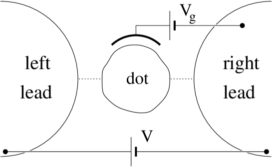
Recent progress in mesoscopic fabrication techniques has made possible not only the creation of more sophisticated devices but also greater control over their properties. Electron systems confined to small space regions, quantum dots, and especially their transport properties have been studied extensively for the last decade [11, 5]. In particular, an individual ultra-small metallic grain of radius less than 5 nm was attached to two leads via oxide tunnel barriers, thus forming a single electron transistor (SET) [11]. Applying bias voltage, $V$, between two leads allows one to study transport properties of the system, Fig. 1.

Figure 1: Scheme of the Coulomb blockade setup.

Alternatively, a SET can be formed by depleting two-dimensional electron gas at the interface of GaAs/AlGaAs heterostructure by applying negative voltages to the metallic surface gates [5].

In this chapter we will assume that the bias voltage is infinitesimally small, $V\to 0$. This corresponds to the linear response regime. In order to tunnel onto the quantum dot, an electron in the left lead has to overcome a charging energy, $E_{C}=e^{2}/2C$, where $e>0$ is the elementary charge; $C$ is the capacitance of the quantum dot. If $T\ll E_{C}$ then conductance through the system is exponentially suppressed. This phenomenon is called the Coulomb blockade. However if we apply a voltage, $V_{g}$, to the additional gate capacitively coupled to the dot, the Coulomb blockade can be lifted. Indeed, changing $V_{g}$ one can shift the position of energy minimum so that energies of the quantum dot with $N_{e}$ and $N_{e}+1$ electrons will become equal and an electron can freely jump from the left lead onto the dot and then jump out into the other lead. Thus, current event has occurred and a peak in the conductance, $G$, corresponding to this gate voltage is observed. By changing the gate voltage one can observe an oscillation of the conductance or Coulomb blockade oscillations.

One-particle energy levels in the quantum dot, $\{E_{i}\}$, are given by the solution of the Schrödinger equation in the quantum dot’s potential. The mean spacing between these energy levels is $\delta E$. The conventional assumption that $E_{C}\gg\delta E$ is not valid in the case of sufficiently small dots. In fact, in the recent experiments [25, 26, 27], where a $C_{60}$ molecule has acted as a quantum dot, the level spacing is of order charging energy. Experiment [25, 26] was performed at $T=4.2K$ as well as at room temperature. In other experiments [28, 29] with quantum dot formed by depleting 2DEG [28] and ropes of carbon nanotubes acting as a quantum dot [29], charging energy is only three times larger than the spacing $\delta E$.

Though Coulomb blockade oscillations have been studied in a number of important limiting cases [30, 31, 32, 33], the problem in the case when values of $E_{C}$, $\delta E$, and $T$ are all of the same order has not been theoretically addressed. Let us note that energy levels of the quantum dots are random and obey Wigner-Dyson statistics with the fluctuation of order of their mean [18]. Nonetheless to go as far as possible in the analytical treatment of the problem we have to assume that energy levels in the quantum dot are equidistant. In this chapter we derive an analytical expression for the linear conductance, $G=I/V|_{V\to 0}$, in the case of spinless as well as spin-$\frac{1}{2}$ fermions.

In Section 3 we describe our model and the assumptions involved. We write the model assuming spin-$\frac{1}{2}$ fermions. In Section 4 we consider the linear conductance in the case of spinless fermions. We obtain an analytical expression for the conductance and analyze its limiting cases. In Section 5 we consider one possible application of the Section 4 results, namely tunneling through the edge states in a quantum dot placed into a strong magnetic field. In Section 6 the linear conductance as well as its properties in the case of spin-$\frac{1}{2}$ fermions is considered. In Section 7 we summarize our findings.

3 The Model

Hamiltonian of the system in question is

$${\hat{H}}={\hat{H}_{l}}+{\hat{H}_{d}}+{\hat{T}}.$$ (1)

Here, the first term is the Hamiltonian of noninteracting electrons in the left and right leads:

$${\hat{H}_{l}}=\sum_{k\sigma}E_{k}c_{k\sigma}^{\dagger}c_{k\sigma}+\sum_{p\sigma}E_{p}c_{p\sigma}^{\dagger}c_{p\sigma},$$ (2)

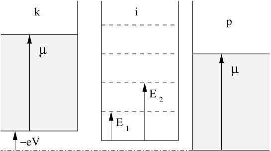
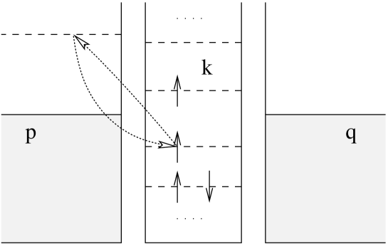
where a continuum of states in each lead, $\left|k\sigma\right>$, $\left|p\sigma\right>$ is assumed; $E_{k}$, $E_{p}$ and $c_{k\sigma}$, $c_{p\sigma}$ are the energies and electron annihilation operators in the left and right leads, respectively; $\sigma$ stands for the $z$-component of spin. The chemical potentials of the leads, $\mu\gg E_{C},\delta E,T$, are shifted according to the bias voltage, $V$, applied, Fig. 2. We will assume that leads are in thermal equilibrium at temperature $T$ and, thus, occupied according to the Fermi-Dirac distribution.

Figure 2: Electrostatic potential energy along a line through the tunnel junctions.

The second term in Eq. (1) is the Hamiltonian of the quantum dot:

$${\hat{H}_{d}}=\sum_{i\sigma}E_{i}c_{i\sigma}^{\dagger}c_{i\sigma}+{\hat{U}},$$ (3)

where first term is the kinetic energy of electrons in the quantum dot: $\{E_{i}\}$ is a discrete set of the quantum dot’s energy levels; $c_{i\sigma}$’s are the annihilation operators. The second term, ${\hat{U}}$ describes the electron-electron interaction in the quantum dot. We adopt the simplest model for the interaction, namely, the constant interaction model. In this model the Coulomb interaction of the electrons depends only on the total number of electrons in the quantum dot:

$$U({\hat{N}})=E_{C}{\hat{N}}^{2}-eV_{e}{\hat{N}},$$ (4)

where $N=\sum_{i\sigma}c_{i\sigma}^{\dagger}c_{i\sigma}-N_{i}$ is the total number of excess electrons; $N_{i}$ is the total number of positively charged ions. The second term is the contribution from external charges. They are supplied by the ionized donors and the gate: $V_{e}=V_{d}+aV_{g}$, where $a$ is a function of the capacitance matrix elements of the system. Thus, $V_{e}$ can be varied continuously by changing gate voltage, $V_{g}$. $U(N)$ can be rewritten as

$$U(N)=E_{C}(N-N_{g})^{2}+\mbox{Const},$$ (5)

where $N_{g}=eV_{e}/2E_{C}$ is the dimensionless gate voltage.

The third term in Eq. (1) is the tunneling Hamiltonian:

$${\hat{T}}=\sum_{ki\sigma}\left(t_{ki}{c}_{k\sigma}^{\dagger}{c}_{i\sigma}+h.c.\right)+\sum_{pi\sigma}\left(t_{pi}{c}_{p\sigma}^{\dagger}{c}_{i\sigma}+h.c.\right),$$ (6)

where $t_{ki}$ and $t_{pi}$ are matrix elements of tunneling into the left and right leads, respectively.

We assume that the dot is weakly coupled to the leads; that is, the conductances of the dot-lead junctions are small: $G^{l,r}\ll e^{2}/h$, where $h$ is Planck’s constant. Equivalently, the widths of the quantum dot’s energy levels contributing to the conductance, $\Gamma_{i}=\Gamma_{i}^{l}+\Gamma_{i}^{r}$, must be small compared to spacing between them: $\Gamma_{i}\ll\delta E$. This, together with $\Gamma_{i}\ll T$ assumption, allows us to characterize the state of the dot by a set of occupation numbers, $\{n_{i\sigma}\}$ [33].

4 Linear Conductance in the Spinless Case

The model formulated above has been studied by Beenakker in the sequential tunneling approximation [33]; that is, conservation of energy was assumed in each tunneling process, and cotunneling was neglected. Therefore, to find the stationary current, kinetic equation considerations can be applied. In the linear response regime an analytical formula for the conductance has been obtained. In the case of spinless fermions [33]:

$$G = \frac{e^{2}}{hT}\sum_{i=1}^{\infty}\frac{\Gamma_{i}^{l}\Gamma_{i}^{r}}{\Gamma_{i}^{l}+\Gamma_{i}^{r}}\sum_{N_{e}=1}^{\infty}P_{eq}(N_{e})F_{eq}(E_{i}|N_{e})$$ (7)

$$\times[1-n_{F}(E_{i}-\mu+U(N)-U(N-1)],$$

where

$$\Gamma_{i}^{l}=2\pi\sum_{k}|t_{ki}|^{2}\delta\left[E_{i}-E_{k}+U(N)-U(N-1)\right]$$

and

$$\Gamma_{i}^{r}=2\pi\sum_{p}|t_{pi}|^{2}\delta\left[E_{i}-E_{p}+U(N)-U(N-1)\right]$$

are widths of the quantum dot’s level $i$ associated with tunneling into the left and right leads, respectively; $P_{eq}(N_{e})$ is the equilibrium probability that the quantum dot contains $N_{e}$ electrons; $F_{eq}(E_{i}|N_{e})$ is the occupation number of level $i$ given that the dot contains $N_{e}$ electrons; $n_{F}(E)$ is the Fermi-Dirac distribution; and $\mu$ is the chemical potential in the leads.

The quantity $F_{eq}(E_{i}|N_{e})$ in (7) is the most non-trivial one to calculate. It is the occupation number of the level $i$ in the canonical ensemble ($N_{e}$ is fixed). In the limit $\delta E/T\to 0$, $F_{eq}(E_{i}|N_{e})$ becomes a Fermi-Dirac distribution with the appropriately chosen chemical potential: $\tilde{\mu}=(E_{0}+E_{1})/2$, where $E_{0}$ corresponds to the energy of the last occupied energy level at $T=0$, Fig. 3(a); $E_{1}$ corresponds to the energy of the first empty energy level at $T=0$. In the opposite limit $\delta E/T\to\infty$, the Fermi-Dirac distribution with $\tilde{\mu}=(E_{0}+E_{1})/2$ apparently breaks down: the occupation number of level $j=1$, for example, see Fig. 3a, is $n_{1}=e^{-\delta E/T}$, not $e^{-\delta E/2T}$ as the Fermi-Dirac distribution would predict [33].

Figure 3: a) occupation numbers in the canonical ensemble for the equidistant energy levels at $T=0$; b) mapping sum over $i$ onto sum over $j$ ($N=2$ case is shown).

The occupation number in question is [33]

$$F_{eq}(E_{i}|N_{e}) = \frac{1}{P_{eq}(N_{e})}\sum_{\{n_{l}\}}P_{eq}(\{n_{l}\})\delta_{n_{i},1}\delta_{N_{e},\sum n_{l}}$$ (8)

$$= e^{\beta F(N_{e})}\sum_{\{n_{l}\}}e^{-\beta\sum E_{l}n_{l}}\delta_{n_{i},1}\delta_{N_{e},\sum n_{l}},$$

where $P_{eq}(\{n_{l}\})$ is the equilibrium probability of the $\left|\{n_{l}\}\right>$ state of the quantum dot; $\beta=1/T$; and the detailed definition of $F(N_{e})$ will follow. The reason for writing this equation is to show that analytical calculation of the occupation numbers is hardly possible for arbitrary quantum dot’s energy level structure, $\{E_{i}\}$.

The only way to overcome this difficulty is to assume that energy levels in the quantum dot are equidistant. Then one can use the bosonization technique [34] (see Appendix 8) to find the exact analytical expression for the occupation numbers in the canonical ensemble. It was done by Denton, Muhlschlegel, and Scalapino [35]:

$$F_{eq}(E_{i}|N_{e})\equiv n_{j}=\sum_{m=1}^{\infty}(-1)^{m-1}e^{-\frac{1}{2}[m^{2}+(2j-1)m]\frac{\delta E}{T}},$$ (9)

where

$$j=\frac{E_{i}-\zeta}{\delta E}+\frac{1}{2}=\mbox{integer},$$ (10)

$\delta E/T\equiv\delta=\mbox{const}$, $\zeta$ is the energy corresponding to the highest occupied energy level at $T=0$ plus $\delta E/2$, Fig. 3(a). This quantity $\zeta$ is somewhat similar to the chemical potential of a dot, though, strictly speaking, the chemical potential is not well-defined for a dot in the canonical ensemble. The difference, $\zeta-\mu$, is a linear function of the gate voltage. Therefore, by properly adjusting “zero” value of the gate voltage it can be put to zero. Hereinafter, we assume that $\zeta-\mu=0$.

To calculate the conductance we also need to know $P_{eq}(N_{e})$, the probability that the dot, in thermodynamic equilibrium with the reservoirs, contains $N_{e}$ electrons. It can be calculated in the grand canonical ensemble:

$$P_{eq}(N_{e})=\frac{1}{Z_{\mu}}e^{-\beta\varphi(N_{e})},$$ (11)

where $Z_{\mu}=\sum_{N_{e}=0}^{\infty}e^{-\beta\varphi(N_{e})}$ is the grand partition function; $\varphi(N_{e})$ is the thermodynamic potential of the quantum dot. It can be expressed via free energy of the dot’s internal degrees of freedom, $F(N_{e})$:

$$\varphi(N_{e})=F(N_{e})-\mu N_{e}+U(N),$$ (12)

hence,

$$P_{eq}(N_{e})=\frac{1}{Z_{\mu}}e^{-\beta U(N)}Z(N_{e}),$$ (13)

where

$$Z(N_{e})=e^{-\beta[F(N_{e})-\mu N_{e}]}=\sum\limits_{\{n_{i}\}}e^{-\beta\sum(E_{i}-\mu)n_{i}}\delta_{N_{e},\sum n_{i}}$$

is the partition function in the canonical ensemble. In the last expression the sum is taken over all possible states, $\left|\{n_{i}\}\right>$ of the quantum dot. To calculate $Z(N_{e})$ explicitly we need to assume that energy levels of the dot are equidistant:

$$Z(N_{e})=e^{-(N_{e}-N_{i})^{2}\delta/2}Z_{exc},$$ (14)

where $N_{e}=N_{i}$ corresponds to the equilibrium number of the excess electrons $(\zeta=\mu)$; $Z_{exc}$ is the partition function of the thermal excitations. Now, let us substitute Eq. (14) in Eq. (13):

$$P_{eq}(N_{e}) = \frac{1}{Z_{\mu}}e^{-\beta U(N)}e^{-(N_{e}-N_{i})^{2}\delta/2}Z_{exc}$$ (15)

$$= \frac{1}{D^{\prime}_{0}}e^{-\beta[U(N)+N^{2}\delta E/2]},$$

where

$$D^{\prime}_{0}=\sum_{N=-\infty}^{\infty}e^{-\beta[U(N)+N^{2}\delta E/2]}.$$ (16)

Here, we have extended one limit of the sum to infinity since the Fermi energy is the largest energy scale of the problem.

Thus, we are well-equipped to calculate the conductance in the case of equidistant energy levels in the quantum dot at arbitrary ratio $\delta$. The widths of energy levels, $\Gamma_{i}^{l}$ and $\Gamma_{i}^{r}$, in the quantum dot are energy dependent, random quantities. Let us assume that quantum dot is weakly coupled to the leads via multichannel tunnel junctions: $G^{l,r}=G^{l,r}_{1}N_{ch}\ll e^{2}/h$, where $N_{ch}$ is the number of channels; $G^{l,r}_{1}$ is the conductance of one channel. Experimentally, this situation corresponds to the metallic grain coupled to the leads via oxide tunnel barriers [11]. This setup allows one to decrease fluctuations of the energy levels’ widths, $\Gamma_{i}^{l}$ and $\Gamma_{i}^{r}$, by a factor of $\sqrt{N_{ch}}$. We also assume that the widths are slowly changing functions of the energy, $E_{i}$. Then, $\Gamma_{i}^{l}$ and $\Gamma_{i}^{r}$ can be considered constants and evaluated at the chemical potential: $\Gamma_{i}^{l}\approx\Gamma_{\mu}^{l}\equiv\Gamma^{l}$; $\Gamma_{i}^{r}\approx\Gamma_{\mu}^{r}\equiv\Gamma^{r}$. There is a simple relation between these widths and conductances of the corresponding junctions. In the case of spinless fermions:

$$\Gamma^{l}=\frac{hG^{l}}{e^{2}}\delta E,~{}~{}~{}\Gamma^{r}=\frac{hG^{r}}{e^{2}}\delta E.$$ (17)

Let us substitute Eq. (15) in Eq. (7):

$$G = \frac{G^{l}G^{r}}{G^{l}+G^{r}}\frac{\delta}{D^{\prime}_{0}}\sum_{N}e^{-\beta[U(N)+N^{2}\delta E/2]}\sum_{i}F_{eq}(E_{i}|N_{e})$$ (18)

$$\times\left\{1-n_{F}\left[E_{i}-\mu+U(N)-U(N-1)\right]\right\}.$$

To take advantage of the expression for occupation numbers, Eq. (9), we need to map the sum over $i$ onto the sum over $j$. As illustrated in Fig. 3, the mapping rule depends on the total number of excess electrons, $N$ (compare with Eq. (10) written for $N=0$):

$$F_{eq}(E_{i}|N_{e}) = n_{j},$$

$$E_{i}-\mu=E_{i}-\zeta^{\prime}+(\zeta^{\prime}-\zeta) = \left(j-\frac{1}{2}\right)\delta E+N\delta E,$$

where $\zeta^{\prime}=\zeta^{\prime}(N)$ is the energy of the highest occupied energy level in the dot with $N$ excess electrons at $T=0$ plus $\delta E/2$. We will also use the following identities:

$$U(N)+\frac{\delta E}{2}N^{2}=\left(E_{C}+\frac{\delta E}{2}\right)N^{2}-eV_{e}N$$

$$=\left(E_{C}+\frac{\delta E}{2}\right)\left(N-\Delta_{0}+\frac{1}{2}\right)^{2}+{\mathcal{C}}_{1},$$ (19)

where ${\mathcal{C}}_{1}=-\left(eV_{e}\right)^{2}/2(2E_{C}+\delta E)$;

$$\Delta_{0}\equiv\frac{eV_{e}}{2E_{C}+\delta E}+\frac{1}{2}$$ (20)

has been chosen so that $\Delta_{0}=0$ corresponds to the maximum of the conductance peak; and

$$U(N)-U(N-1)=(2N-1)E_{C}-eV_{e}$$

$$=(2N-1)E_{C}-(2E_{C}+\delta E)(\Delta_{0}-1/2).$$ (21)

Substituting these results in Eq. (18), we obtain

$$\frac{G(\Delta_{0})}{G_{\infty}}=\frac{\delta}{D_{0}}\sum_{N}e^{-\varepsilon_{0}\left(N-\Delta_{0}+\frac{1}{2}\right)^{2}}\sum_{j}\frac{n_{j}}{e^{-j\delta-2(N-\Delta_{0})\varepsilon_{0}}+1},$$ (22)

where

$$D_{0}=\exp\left(\beta{\mathcal{C}}_{1}\right)D^{\prime}_{0}=\sum_{N}e^{-\varepsilon_{0}\left(N-\Delta_{0}+\frac{1}{2}\right)^{2}};$$ (23)

$\varepsilon_{0}\equiv\beta(E_{C}+\delta E/2)$; $G_{\infty}\equiv G^{l}G^{r}/(G^{l}+G^{r})$ is the classical, $E_{C},\delta E\ll T\ll\mu$, limit of the conductance. We have also used the identity: $1-n_{F}(E)=(1+e^{-\beta E})^{-1}$. Eq. (22) is the general expression for the linear conductance in the spinless case for equidistant energy levels in the quantum dot at arbitrary values of $E_{C}$, $\delta E$ and $T$.

One can immediately prove the following properties of the conductance, Eq. (22). First of all, $G(\Delta_{0})=G(\Delta_{0}+M)$, where $M$ is an integer. In the gate voltage units, $\Delta V_{e}=(2E_{C}+\delta E)/e$ is a period of the conductance oscillations. This property reflects symmetry with respect to adding (removing) an electron to the quantum dot. Secondly, due to the electron-hole symmetry, conductance is an even function of $\Delta_{0}$: $G(\Delta_{0})=G(-\Delta_{0})$.

Figure 4: Coulomb blockade oscillations of the conductance as a function of the dimensionless gate voltage, $\Delta_{0}$ at $\delta E=E_{C}$. Curves are plotted for different temperatures: $T/E_{C}=T/\delta E\equiv 1/\delta=0.2,0.35,0.5,0.7,1,2,5$.

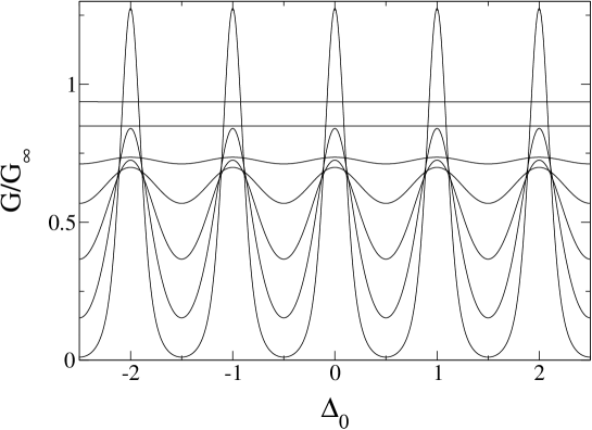
The linear conductance, Eq. (22), as a function of the dimensionless gate voltage $\Delta_{0}$ at $\delta E=E_{C}$ is plotted in Fig. 4 for different temperatures. At low temperatures there are sharp Coulomb blockade peaks. At high temperatures, $T\gg E_{C},\delta E$, Coulomb blockade is lifted and small oscillations of the conductance can be observed. These oscillations are slightly non-sinusoidal and given by the following asymptotic formula:

$$\frac{G(\Delta_{0})-\overline{G(\Delta_{0})}}{G_{\infty}}=2\pi^{3/2}\frac{e^{-\varepsilon_{0}/4}}{\sqrt{\varepsilon_{0}}}\left[e^{-\pi^{2}/\varepsilon_{0}}\cos(2\pi\Delta_{0})\right.$$

$$+\left.e^{-2\pi^{2}/\varepsilon_{0}}\cos(4\pi\Delta_{0})+O(e^{-3\pi^{2}/\varepsilon_{0}})\right],$$ (24)

where $\overline{G(\Delta_{0})}$ is the average value of the conductance. The second term in Eq. (24) is due to inherently non-sinusoidal nature of the conductance oscillations, see Fig. 4. To derive this expression one can use Poisson’s summation formula.

Figure 5: The exact line shape of the conductance peak, Eq. (26), plotted at $1/\delta\equiv T/\delta E=0.4$ (solid curve). Dotted curve corresponds to blindly applying classical regime formula (27) at $T/\delta E=0.4$. Dashed curve corresponds to blindly applying formula (28) at $T/\delta E=0.4$. The argument of the plot is linear function of the gate voltage, $\phi_{0}$.

To study the line shape of a separate peak let us consider the limit of large charging energy: $E_{C}\gg T,\delta E$ or, equivalently, $\varepsilon_{0}\gg 1,\delta$ in the dimensionless units. In Eq. (22) only $N=-1,0$ terms in the sum over $N$ give substantial contribution to the conductance near $\Delta_{0}=0$; all other terms are exponentially suppressed. Besides, the sum over $j$ at the $N=-1$ is $O(e^{-2\varepsilon_{0}})$ and, therefore, can also be neglected. Hence, line shape of the conductance peak at $\Delta_{0}=0$ is given by

$$\frac{G(\Delta_{0})}{G_{\infty}}=\frac{\delta}{1+e^{-2\varepsilon_{0}\Delta_{0}}}\sum_{j}\frac{n_{j}}{1+e^{-j\delta+2\varepsilon_{0}\Delta_{0}}}.$$ (25)

It is more instructive to rewrite this equation as follows:

$$\frac{G(\phi_{0})}{G_{\infty}}=\frac{\delta}{1+e^{-\beta e\phi_{0}}}\sum_{j}\frac{n_{j}}{1+e^{-j\delta+\beta e\phi_{0}}},$$ (26)

where $\phi_{0}=V_{e}-V_{e}^{(0)}$; $V_{e}^{(0)}$ is chosen so that $\phi_{0}=0$ corresponds to center of the conductance peak. In the classical regime [30], $T\gg\delta E$, line shape of the conductance peak is given by

$$\frac{G(\phi_{0})}{G_{\infty}}=\frac{\beta e\phi_{0}}{2\sinh(\beta e\phi_{0})}.$$ (27)

In the opposite limit of $\delta E\gg T$:

$$\frac{G(\phi_{0})}{G_{\infty}}=\frac{\delta}{2[1+\cosh(\beta e\phi_{0})]}.$$ (28)

The exact line shape of the conductance peak, Eq. (26), at $T/\delta E=0.4$ is shown in Fig. 5. On the same figure we also plotted two conductance peaks in the limiting cases, Eqs. (27) and (28), out of their validity region at $T/\delta E=0.4$. Nevertheless, it is interesting that the exact conductance peak is higher than both of the limiting cases peaks. The peak’s height is given by

$$\frac{G(0)}{G_{\infty}}=\frac{\delta}{2}\sum_{j}\frac{n_{j}}{1+e^{-j\delta}}=\left\{\begin{array}[]{l}1/2,~{}~{}T\gg\delta E\\ \delta/4,~{}~{}\delta E\gg T\gg\Gamma_{i}\end{array}\right..$$ (29)

Temperature dependence of the conductance peak’s height was numerically calculated in the Ref. [33], see Fig. 2 there.

5 Application to Tunneling Through Quantum Hall Edge States in a Quantum Dot

Formulas for the linear conductance in the case of equidistant energy levels in a dot and spinless fermions derived in Section 4 can be applied to a number of physical problems.

Let us consider, for example, a quantum dot formed by confining a two-dimensional electron gas by a circularly symmetric electrostatic potential, $U(r)$. We assume that $U(r)$ is zero at the origin and takes large value at $r=R$, where $R$ is the radius of the dot, Fig. 6(a). Let us apply a strong magnetic field, $B$, perpendicular to the plane of the dot. This situation corresponds to the quantum Hall regime and was reviewed in Ref. [36].

Figure 6: Geometry and spectrum of the quantum dot states: a) symmetric gauge eigenstates, $\left|m\right>$, including edge state are shown schematically; b) energy spectrum of the eigenstates with different angular momenta, two lowest Landau levels are shown.

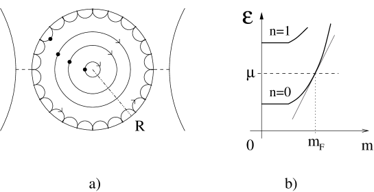
To solve the one-electron Schrödinger equation in this geometry it is convenient to choose the symmetric gauge. Then, angular momentum is, clearly, an integral of motion. In each Landau level, $n$, states with larger angular momentum, $\left|m\right>$, are localized further from the origin, near a circle with radius $R_{m}=l_{H}\sqrt{2(m+1)}$, where $l_{H}=\sqrt{\hbar c/eB}$ is the magnetic length, $c$ is the speed of light. The presence of the confinement potential leads to an increase in energy for the symmetric gauge eigenstates with $R_{m}$ of order or larger than $R$ (or, $m$ of order or larger than $m_{F}$, see Fig. 6(b)). For the states with $R_{m}\sim R$ an electron is influenced by both the electric field of the boundary, $E(R)=U^{\prime}(R)/e$, and strong, perpendicular to the electric, magnetic field. Thus, near the edge electron executes rapid cyclotron orbits centered on a point that slowly drifts in the direction of ${\bf E}\times{\bf B}$, that is, along the boundary. Thus, Quantum Hall edge states are formed, Fig. 6(a). It is important to notice that in this closed geometry electron system has only one edge. In this consideration we also assume that $l_{H}\ll R$.

For simplicity let us consider the case when only the zeroth Landau level crosses the chemical potential, that is, there is only one type of edge states. This corresponds to a sufficiently strong magnetic field so that filling factor, $\nu$ is equal to $1$, Fig. 6(b).

Now, we are ready to consider transport through this type of quantum dot in the strong magnetic field. Let us weakly couple it to two leads and apply an infinitesimally small bias voltage between them. An electron from the left lead can now tunnel into dot’s edge state and then tunnel into the right lead as illustrated by dashed lines in Fig. 6(a).

The energy spectrum of edge states can be linearized as follows

$${\mathcal{E}}_{m}=\mu+\left.\frac{\partial{\mathcal{E}}}{\partial m}\right|_{m_{F}}\left(m-m_{F}\right).$$ (30)

Thus, energy levels of the edge states are equally spaced with the spacing [36]

$$\delta E=\left.\frac{\partial{\mathcal{E}}_{m}}{\partial m}\right|_{m_{F}}=\left.\frac{\partial{\mathcal{E}}_{m}}{\partial R_{m}}\right|_{R}\left.\frac{\partial R_{m}}{\partial m}\right|_{m_{F}}=eE(R)\frac{l_{H}^{2}}{R}.$$ (31)

This fact makes formulas derived in Section 4 applicable to this problem. Essential assumption here is that dispersion curve, Fig. 6(b) is almost linear in the range of angular momentums: $|m-m_{F}|\lesssim\Delta m$, where $\Delta m=\mbox{max}(1,T/\delta E)$.

In the case at hand, spacing, $\delta E$ is inversely proportional to the size of a dot just like charging energy, $E_{C}$. Hence, their ratio does not depend on the size of a dot and is given by

$$\frac{\delta E}{E_{C}}\sim\frac{\epsilon}{\alpha}\frac{E(R)}{B},$$ (32)

where $\epsilon$ is the dielectric constant of the media around the interface; $\alpha=e^{2}/\hbar c$ is the fine structure constant. Therefore, in this case oscillations of the conductance given by Eq. (22) are determined by only one parameter $\delta=\delta E/T$.

In conclusion, let us consider the case of an arbitrary shaped quantum dot. In this case, $m$ is just the index of an edge state and no longer associated with the angular momentum. The phase along the boundary for the $m$-th edge state is

$$\theta_{m}=\int_{0}^{L}dx~{}k_{m}(x),$$ (33)

where $k_{m}(x)$ is the corresponding wave vector, $x$ parametrizes the boundary, and $L$ is its length. The phase difference between two consecutive edge states is

$$\theta_{m+1}-\theta_{m}=2\pi=\int_{0}^{L}dx\left[k_{m+1}(x)-k_{m}(x)\right],$$ (34)

where $k_{m+1}(x)-k_{m}(x)=\left({\mathcal{E}}_{m+1}-{\mathcal{E}}_{m}\right)/\hbar v(x)$, $v(x)=cE(x)/B$ is a drift speed along the boundary. Then, the spacing between edge states’ energy levels is

$$\delta E=2\pi\hbar\left[\int_{0}^{L}\frac{dx}{v(x)}\right]^{-1}=2\pi el_{H}^{2}\left[\int_{0}^{L}\frac{dx}{E(x)}\right]^{-1}.$$ (35)

Though the electric field $E(x)$ at the boundary slightly changes as one goes from one edge state to the other, this effect is small and we neglect it. Therefore, the energy levels of the edge states are equidistant with the spacing given by Eq. (35).

In the case of the circularly symmetric quantum dot, $E(x)$ is constant, and one can easily perform the integration in Eq. (35). This leads to the previously obtained expression for the level spacing, Eq. (31).

6 Linear Conductance in the Spin-$\frac{1}{2}$ Case

Formula (7) for the linear conductance in the spinless case can be easily generalized to the spin-$\frac{1}{2}$ case by counting each energy level twice [33]:

$$G = 2\frac{e^{2}}{hT}\sum_{i=1}^{\infty}\frac{\Gamma_{i}^{l}\Gamma_{i}^{r}}{\Gamma_{i}^{l}+\Gamma_{i}^{r}}\sum_{N_{e}=1}^{\infty}P_{eq}(N_{e})F_{eq}(E_{i\uparrow}|N_{e})$$ (36)

$$\times[1-n_{F}(E_{i}-\mu+U(N)-U(N-1))],$$

where $F_{eq}(E_{i\uparrow}|N_{e})$ is the occupation number of the quantum dot’s energy level $i$ with a spin-up electron, ($i,\uparrow$) in the canonical ensemble: number of electrons in the dot, $N_{e}$, is fixed.

As in the spinless case, to carry out analytical consideration we have to assume that energy levels in the quantum dot are equally spaced. Presence of the spin degeneracy makes the calculations more complicated.

First of all, let us find the occupation number $F_{eq}(E_{i\uparrow}|N_{e})$. Let us consider spin-up and spin-down electron subsystems. Ground state energy of the system is

$$E_{g}=\left(N^{2}_{\uparrow}+N^{2}_{\downarrow}\right)\frac{\delta E}{2}=\left[\left(N_{\uparrow}+N_{\downarrow}\right)^{2}+\left(N_{\uparrow}-N_{\downarrow}\right)^{2}\right]\frac{\delta E}{4},$$

where $N_{\sigma}=(N_{e})_{\sigma}-N_{i}/2$ is the number of excess electrons in the spin-$\sigma$ subsystem; $N_{i}$ is chosen even. $N_{\uparrow}+N_{\downarrow}\equiv N$ is the total number of excess electrons in the quantum dot; $(N_{\uparrow}-N_{\downarrow})/2\equiv S_{z}$ is $z$-component of the total electron spin. Using these identities, one can find that

$$E_{g}=\frac{1}{4}N^{2}\delta E+S_{z}^{2}\delta E.$$ (37)

While $S_{z}$ is subjected to the thermodynamic fluctuations, $N$ is fixed.

Figure 7: Parameter $\zeta^{\prime}$ of the spin-up electron subsystem for even number of electrons: a) at $S_{z}=0$, b) at arbitrary integer $S_{z}$ ($S_{z}=1$ case is shown); for odd number of electrons: c) at $S_{z}=1/2$, d) at arbitrary half-integer $S_{z}$ ($S_{z}=3/2$ case is shown).

The occupation number in question, $F_{eq}(E_{i\uparrow}|N_{e})\equiv n_{j\uparrow}$, is known if, in addition to $N$, the $z$-component of the total spin, $S_{z}$, is fixed. In the case of an even number of electrons, parameter $\zeta^{\prime}$ for the spin-up electron subsystem is equal to $\zeta+S_{z}\delta E$, given $S_{z}$, see Figs. 7(a) and 7(b). Occupation numbers in the spin-up subsystem at fixed $S_{z}$ are given by Eq. (9) with the appropriately chosen parameter $\zeta^{\prime}$: $n_{j-S_{z}}$.

However, $z$-component of the total spin, $S_{z}$, is not fixed but subjected to the thermodynamic fluctuations. Therefore, to find the occupation numbers, $n_{j\uparrow}^{ev}$, we have to account for all possible values of $S_{z}$:

$$n_{j\uparrow}^{ev}=\sum_{S_{z}=-N_{e}/2}^{N_{e}/2}P(S_{z})~{}n_{j-S_{z}},$$ (38)

where

$$P(S_{z})=\frac{e^{-S_{z}^{2}\delta}}{\sum\limits_{S_{z}=-N_{e}/2}^{N_{e}/2}e^{-S_{z}^{2}\delta}}$$ (39)

is the probability that $z$-component of the total spin of the quantum dot is equal to $S_{z}$. Substituting Eqs. (39) and (9) into Eq. (38) we obtain

$$n_{j\uparrow}^{ev}=\sum\limits_{m=1}^{\infty}(-1)^{m-1}e^{-\left[m^{2}+(2j-1)m\right]\frac{\delta}{2}}~{}\frac{\sum\limits_{S_{z}=-N_{e}/2}^{N_{e}/2}e^{-\left(S_{z}^{2}-mS_{z}\right)\delta}}{\sum\limits_{S_{z}=-N_{e}/2}^{N_{e}/2}e^{-S_{z}^{2}\delta}}.$$

Since number of electrons in the quantum dot is even, $S_{z}$ may take only integer values. Therefore,

$$n_{j\uparrow}^{ev}=\sum\limits_{m=1}^{\infty}(-1)^{m-1}e^{-\left[\frac{m^{2}}{4}+(j-\frac{1}{2})m\right]\delta}~{}\frac{\sum\limits_{S_{z}=-\infty}^{\infty}e^{-(S_{z}-\frac{m}{2})^{2}\delta}}{\sum\limits_{S_{z}=-\infty}^{\infty}e^{-S_{z}^{2}\delta}},$$

where we extended limits of the sum over $S_{z}$ to infinities since the Fermi energy is the largest energy scale in the problem. Separating $m=2r-1$ and $m=2r$ parts of the sum, where $r$ is a positive integer, we obtain final expression for the occupation numbers in the case of even number of electrons:

$$n_{j\uparrow}^{ev}=A(\delta)\sum_{r=1}^{\infty}e^{-(r-\frac{1}{2})(r+2j-\frac{3}{2})\delta}-\sum_{r=1}^{\infty}e^{-r(r+2j-1)\delta},$$ (40)

where

$$A(\delta) = \frac{\sum\limits_{s=-\infty}^{\infty}e^{-\left(s-\frac{1}{2}\right)^{2}\delta}}{\sum\limits_{s=-\infty}^{\infty}e^{-s^{2}\delta}}.$$ (41)

In two limiting cases

$$A(\delta) = \left\{\begin{array}[]{l}2e^{-\delta/4}\left[1+O\left(e^{-\delta}\right)\right],~{}~{}\delta E\gg T\\ \\ 1-4e^{-\pi^{2}/\delta}+O\left(e^{-2\pi^{2}/\delta}\right),~{}~{}T\gg\delta E\end{array}\right..$$

Analytical expression for the high-temperature limit of $A(\delta)$ can be obtained using Poisson’s summation formula.

One can easily prove the following properties of the occupation numbers $n_{j\uparrow}^{ev}$ valid at arbitrary temperature:

$$n_{j\uparrow}^{ev} = 1-n_{1-j,\uparrow}^{ev},$$ (45)

$$e^{j\delta}n_{j\uparrow}^{ev}+e^{-j\delta}n_{-j\uparrow}^{ev} = A(\delta)e^{\delta/4}.$$ (46)

They are valid due to the electron-hole symmetry and similar to the following properties of the Fermi-Dirac distribution: $n_{F}(E)=1-n_{F}(-E)$ and $e^{\beta E}n_{F}(E)+e^{-\beta E}n_{F}(-E)$ $=1$.

Similarly, one can find occupation numbers in the case of odd number of electrons in the quantum dot, $N_{e}$. Energy level which contains one electron at $T=0$ will be referred to as $j=0$ level. In this case electron-hole symmetry corresponds to $j\to-j$ transformation. Parameter $\zeta^{\prime}$ of the spin-up electron subsystem at a given $S_{z}$ is equal to $\zeta+(S_{z}-1/2)\delta E$, see Figs. 7(c) and 7(d). Therefore,

$$n_{j\uparrow}^{od}=\sum\limits_{S_{z}=-N_{e}/2}^{N_{e}/2}P\left(S_{z}\right)~{}n_{j-\left(S_{z}-\frac{1}{2}\right)}$$

$$=\sum\limits_{m=1}^{\infty}(-1)^{m-1}e^{-\left(\frac{m^{2}}{4}+jm\right)\delta}~{}\frac{\sum\limits_{S_{z}=-N_{e}/2}^{N_{e}/2}e^{-\left(S_{z}-\frac{m}{2}\right)^{2}\delta}}{\sum\limits_{S_{z}=-N_{e}/2}^{N_{e}/2}e^{-S_{z}^{2}\delta}}.$$ (47)

Since number of electrons in the quantum dot is odd, $S_{z}$ may take only half-integer values. Separating odd and even parts of the sum over $m$, we obtain:

$$n_{j\uparrow}^{od}=\frac{1}{A(\delta)}\sum_{r=1}^{\infty}e^{-\left(r-\frac{1}{2}\right)\left(r+2j-\frac{1}{2}\right)\delta}-\sum_{r=1}^{\infty}e^{-r(r+2j)\delta}.$$ (48)

Property of the electron-hole symmetry reads as follows: $n_{j\uparrow}^{od}=1-n_{-j\uparrow}^{od}$.

It turns out that there exists simple relation between $n^{ev}$ and $n^{od}$ occupation numbers:

$$n_{j\uparrow}^{ev}=A(\delta)e^{-\left(j-\frac{1}{4}\right)\delta}n_{-j\uparrow}^{od}.$$ (49)

This property is the analog of $n_{F}(E)=e^{-\beta E}n_{F}(-E)$ one of the Fermi-Dirac distribution. It will allow us to get rid of $n^{od}$ occupation numbers in the final expression for the conductance.

Now we are in a position to find the probability that a dot, in thermodynamic equilibrium with the reservoirs, contains $N_{e}$ electrons, $P_{eq}(N_{e})$. Eq. (13) written for the spinless case is still applicable if we keep in mind that energy levels in the quantum dot are doubly degenerate. Partition function of the dot’s internal degrees of freedom in the canonical ensemble is

$${\mathcal{Z}}(N_{e}) = \sum\limits_{\{n_{i\sigma}\}}e^{-\beta\sum(E_{i}-\mu)n_{i\sigma}}\delta_{N_{e},\sum n_{i\sigma}}$$ (50)

$$= \sum\limits_{N_{e}^{\uparrow}=0}^{N_{e}}\sum\limits_{N_{e}^{\downarrow}=0}^{N_{e}}Z(N_{e}^{\uparrow})Z(N_{e}^{\downarrow})\delta_{N_{e},N_{e}^{\uparrow}+N_{e}^{\downarrow}},$$

where

$$Z(N_{e}^{\uparrow})=\sum_{\{n_{i}\}}e^{-\beta\sum(E_{i}-\mu)n_{i}}\delta_{N_{e}^{\uparrow},\sum n_{i}}$$ (51)

is the partition function of the spin-up electron subsystem in the canonical ensemble. Mathematically, expression for $Z(N_{e}^{\uparrow})$ is identical to the one for $Z(N_{e})$ in the spinless case. Thus, one can directly apply the result obtained previously, Eq. (14):

$$Z(N_{e}^{\uparrow})=e^{-(N_{e}^{\uparrow}-N_{i}/2)^{2}\delta/2}Z_{exc},$$ (52)

where $N_{e}^{\uparrow}=N_{i}/2$ is the equilibrium number of electrons in the spin-up subsystem. Similar result is valid for the partition function of the spin-down electron subsystem, $Z(N_{e}^{\downarrow})$. Substituting these results in Eq. (50) we obtain:

$${\mathcal{Z}}(N_{e})=Z_{exc}^{2}\,\sum_{N_{e}^{\uparrow}=0}^{N_{e}}\sum_{N_{e}^{\downarrow}=0}^{N_{e}}e^{-\left[(N_{e}^{\uparrow}-N_{i}/2)^{2}+(N_{e}^{\downarrow}-N_{i}/2)^{2}\right]\delta/2}\delta_{N_{e}^{\uparrow}+N_{e}^{\downarrow},N_{e}}.$$

The exponent can be simplified as follows

$$\left(N_{e}^{\uparrow}-\frac{N_{i}}{2}\right)^{2}+\left(N_{e}^{\downarrow}-\frac{N_{i}}{2}\right)^{2}=\frac{N^{2}}{2}+\frac{\left(N_{e}^{\uparrow}-N_{e}^{\downarrow}\right)^{2}}{2},$$

hence,

$$\frac{{\mathcal{Z}}(N_{e})}{Z_{exc}^{2}} = e^{-N^{2}\delta/4}\sum_{N_{e}^{\uparrow}=0}^{N_{e}}\sum_{N_{e}^{\downarrow}=0}^{N_{e}}e^{-(N_{e}^{\uparrow}-N_{e}^{\downarrow})^{2}\delta/4}\delta_{N_{e}^{\uparrow}+N_{e}^{\downarrow},N_{e}}$$

$$= e^{-N^{2}\delta/4}\sum_{N_{e}^{\uparrow}=0}^{N_{e}}e^{-(N_{e}^{\uparrow}-N_{e}/2)^{2}\delta}=e^{-N^{2}\delta/4}\sum_{s=-N_{e}/2}^{N_{e}/2}e^{-s^{2}\delta},$$

where in the second equality we took advantage of the delta symbol. Sum in the last line is taken over integer values of $s$ if $N_{e}$ is even or half-integer values of $s$ if $N_{e}$ is odd. Limits of the sum over $s$ can be extended to infinities since we assume that $\mu\gg T$. According to Eq. (13) probability that quantum dot, in thermodynamic equilibrium with the reservoirs, contains $N_{e}$ electrons is

$$P_{eq}(N_{e}) = \frac{{\mathcal{Z}}(N_{e})}{Z_{\mu}}e^{-\beta U(N)}=\frac{Z_{exc}^{2}}{Z_{\mu}}e^{-\beta{\tilde{U}}(N)}\sum_{s=-N_{e}/2}^{N_{e}/2}e^{-s^{2}\delta}$$

$$= \frac{e^{-\beta{\tilde{U}}(N)}\sum\limits_{s=-N_{e}/2}^{N_{e}/2}e^{-s^{2}\delta}}{\sum\limits_{N=ev}e^{-\beta{\tilde{U}}(N)}\sum\limits_{s}e^{-s^{2}\delta}+\sum\limits_{N=od}e^{-\beta{\tilde{U}}(N)}\sum\limits_{s}e^{-\left(s-\frac{1}{2}\right)^{2}\delta}},$$

where ${\tilde{U}}(N)\equiv U(N)+N^{2}\delta E/4$; and we used the fact that $N$ and $N_{e}$ have the same parity since $N_{i}$ is chosen even. Therefore, sums over $N=ev$ and $N=od$ are taken over $N=0,\pm 2,\pm 4,\ldots$ and $N=\pm 1,\pm 3,\ldots$ values, respectively. At this point in the calculation we need to specify whether the total number of electrons in the dot is even or odd:

$$P_{eq}(N_{e})=\left\{\begin{array}[]{l}\left(D^{\prime}\right)^{-1}e^{-\beta{\tilde{U}}(N)},~{}~{}N~{}\mbox{is~{}even}\\ \left(D^{\prime}\right)^{-1}A(\delta)e^{-\beta{\tilde{U}}(N)},~{}~{}N~{}\mbox{is~{}odd}\end{array}\right.,$$ (53)

where

$$D^{\prime}\equiv\sum_{N=even}e^{-\beta{\tilde{U}}(N)}+A(\delta)\sum_{N=odd}e^{-\beta{\tilde{U}}(N)}.$$ (54)

Now we are prepared to calculate the conductance, Eq. (36), in the case of the equidistant double degenerate energy levels in the dot at an arbitrary $\delta E/T$ and $E_{C}/\delta E$ ratios. Similarly to the consideration in the spinless case we assume that quantum dot is weakly coupled to the leads via multichannel tunnel junctions, and tunneling widths of the energy levels in the quantum dot, $\Gamma_{i}^{l}$ and $\Gamma_{i}^{r}$, are slowly changing functions of the energy, $E_{i}$.

Figure 8: Mapping of the sum over $i$ onto the sum over $j$ for a) $N=0$; b) even $N$ ($N=-4$ case is shown); c) odd $N$ ($N=-3$ case is shown).

Then, these tunneling widths can be considered constants and evaluated at the chemical potential: $\Gamma_{i}^{l}\approx\Gamma^{l}_{\mu}\equiv\Gamma^{l}$; $\Gamma_{i}^{r}\approx\Gamma^{r}_{\mu}\equiv\Gamma^{r}$. Furthermore, they can be expressed via conductances of the corresponding junctions:

$$\Gamma^{l}=\frac{hG^{l}}{e^{2}}\frac{\delta E}{2},~{}~{}~{}\Gamma^{r}=\frac{hG^{r}}{e^{2}}\frac{\delta E}{2}.$$ (55)

There is an additional factor of $1/2$ here compared to the spinless case, Eq. (17), due to the double degeneracy of each energy level in the quantum dot. First of all, let us break the sum over $N_{e}$ in Eq. (36) in two parts: $N=even$ and $N=odd$, and apply Eqs. (55) and (53):

$$G=\frac{G^{l}G^{r}}{G^{l}+G^{r}}\frac{\delta}{D^{\prime}}$$

$$\times\left(\sum_{N=even}e^{-\beta{\tilde{U}}(N)}\sum_{i=1}^{\infty}F_{eq}(E_{i\uparrow}|N_{e})\left\{1-n_{F}\left[E_{i}-\mu+U(N)-U(N-1)\right]\right\}\right.$$

$$\left.+A(\delta)\sum_{N=odd}e^{-\beta{\tilde{U}}(N)}\sum_{i=1}^{\infty}F_{eq}(E_{i\uparrow}|N_{e})\left\{1-n_{F}\left[E_{i}-\mu+U(N)-U(N-1)\right]\right\}\right).$$ (56)

To take advantage of the occupation numbers we derived, Eqs. (40) and (48), we need to map each of the sums over $i$ onto the sum over $j$. The first sum over $i$ in Eq. (56) is taken at even number of excess electrons, see Figs. 8(a) and 8(b), hence

$$F_{eq}\left(E_{i\uparrow}|N_{e}\right) = n_{j\uparrow}^{ev},$$

$$E_{i}-\mu=E_{i}-\zeta^{\prime}+\left(\zeta^{\prime}-\zeta\right) = \left(j-\frac{1}{2}\right)\delta E+\frac{1}{2}N\delta E.$$

Remember that by properly choosing “zero” of the gate voltage we put $\zeta=\mu$. The second sum over $i$ is taken at odd number of excess electrons, see Figs. 8(a) and 8(c), therefore

$$F_{eq}\left(E_{i\uparrow}|N_{e}\right) = n_{j\uparrow}^{od},$$

$$E_{i}-\mu=E_{i}-\zeta^{\prime}+\left(\zeta^{\prime}-\zeta\right) = j\delta E+\frac{1}{2}N\delta E.$$

We will also use the following identities:

$${\tilde{U}}(N)=\left(E_{C}+\frac{\delta E}{4}\right)N^{2}-eV_{e}N=\left(E_{C}+\frac{\delta E}{4}\right)\left(N-\Delta+\frac{1}{2}\right)^{2}+{\mathcal{C}}_{2},$$

where ${\mathcal{C}}_{2}=-(eV_{e})^{2}/(4E_{C}+\delta E)$;

$$\Delta\equiv\frac{eV_{e}}{2(E_{C}+\delta E/4)}+\frac{1}{2}$$ (57)

is the dimensionless gate voltage, $\Delta=0$ corresponds to a position of the conductance peak; and

$$U(N)-U(N-1)=(2N-1)E_{C}-eV_{e}=(2N-1)E_{C}-2(E_{C}+\frac{\delta E}{4})(\Delta-\frac{1}{2}).$$

Substituting these results in Eq. (56) we obtain

$$\frac{G(\Delta)}{G_{\infty}} = \frac{\delta}{D}\sum_{N=even}e^{-\varepsilon\left(N-\Delta+1/2\right)^{2}}$$ (58)

$$\times \sum_{j=-\infty}^{\infty}n_{j\uparrow}^{ev}\left[\frac{1}{e^{-(j-1/4)\delta-2(N-\Delta)\varepsilon}+1}+\frac{1}{e^{-(j-1/4)\delta+2(N+1-\Delta)\varepsilon}+1}\right],$$

where

$$D=\exp\left(\beta{\mathcal{C}}_{2}\right)D^{\prime}=\sum_{N=even}e^{-\varepsilon(N-\Delta+1/2)^{2}}+A(\delta)\sum_{N=odd}e^{-\varepsilon(N-\Delta+1/2)^{2}};$$ (59)

$$\varepsilon\equiv\beta\left(E_{C}+\frac{\delta E}{4}\right);$$ (60)

$G_{\infty}\equiv G^{l}G^{r}/(G^{l}+G^{r})$ is the high-temperature, $E_{C},\delta E\ll T\ll\mu$, limit of the conductance. To eliminate $n^{od}$ from the final expression we used useful property of the occupation numbers given by Eq. (49).

Formula (58) is the main result of this chapter. It is the analytical expression for the linear conductance in the spin-$\frac{1}{2}$ case for equidistant energy levels in the quantum dot. One can use Eq. (58) to plot Coulomb blockade oscillations of the conductance as a function of the dimensionless gate voltage, $\Delta$, at arbitrary values of $E_{C}$, $\delta E$ and $T$. Particularly, when all energy scales are of the same order: $E_{C}\sim\delta E\sim T$, numerical calculation is a breeze, Fig. 9.

One can immediately notice the following properties of the linear conductance. First of all, $G(\Delta)=G(\Delta+2M)$, where $M$ is an integer. In other words, $(4E_{C}+\delta E)/e$ is the conductance period in the gate voltage units. This property reflects symmetry with respect to adding (removing) two electrons to (from) the quantum dot. Secondly, conductance is a symmetric function with respect to the center of a valley, $\Delta^{\prime}=M+1/2$, where $M$ is an integer. That is, $G(\Delta-\Delta^{\prime})=G(\Delta^{\prime}-\Delta)$. This is a reflection of the electron-hole symmetry. These properties of the conductance oscillations are not generic. They are valid due to the assumption of equally spaced energy levels in a quantum dot.

Figure 9: Linear conductance oscillations as a function of the dimensionless gate voltage, $\Delta$, at $\delta E=E_{C}$. Curves are plotted for different temperatures: $T/E_{C}=T/\delta E\equiv 1/\delta=0.15,0.3,0.5,0.7,1,2,5$ using Eq. (58).

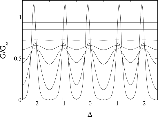
At high temperatures, $T\gg E_{C},\delta E$, conductance peaks overlap and their maximums become almost equidistant, Fig. 9. As a result, instead of separate peaks, the conductance in this limit has oscillatory behavior.

Figure 10: Temperature dependence of the conductance in the odd, $G(-1/2)/G_{\infty}$ and even, $G(1/2)/G_{\infty}$ valleys at $\delta E=E_{C}$. Upper curve corresponds to the conductance in the odd valley.

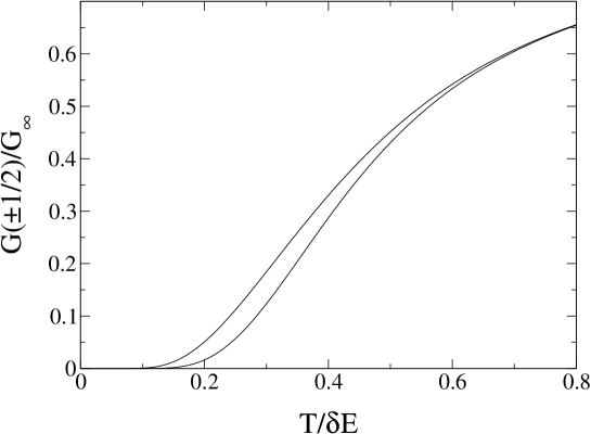
Let us find temperature dependence of the conductance in the valleys. In the sequential tunneling approximation the conductance in the valleys decays exponentially as $T\to 0$, Fig. 10. At low temperature number of electrons in a dot in the valleys is almost quantized. We will call the valley “odd” (“even”) if it corresponds to odd (even) number of electrons in the dot. We find that at any temperature the conductance in the odd valley is larger than that in the even one, Fig. 10. This feature is robust with respect to the distribution of energy levels in a quantum dot.

However, it is important to mention that at low temperatures, $T<T_{in}$, where

$$T_{in}\simeq\frac{E_{C}}{\ln\left(\frac{e^{2}/\hbar}{G^{l}+G^{r}}\right)}$$ (61)

cotunneling [9] will dominate sequential tunneling contribution to the conductance in the valleys. Therefore, temperature dependence of the conductance in the valleys, Fig. 10, is valid only for the temperatures $T>T_{in}$.

Let us analyze the limit of large charging energy: $E_{C}\gg T,\delta E$ or, equivalently, $\varepsilon\gg 1,\delta$ in the dimensionless units. In this limit, two adjacent peaks in the conductance have exponentially small, $\sim e^{-E_{C}/T}$, overlap with each other. Thus, it makes perfect sense to study the line shape of a separate peak. Let us determine line shape of the conductance peak near $\Delta=0$. In the numerator of Eq. (58) only the $N=0$ term in the sum over $N$ survives; moreover, at $N=0$ second term in square brackets is $O(e^{-2\varepsilon})$. In the denominator, only the $N=-1,0$ terms matter. Hence, the line shape of the conductance peak near $\Delta=0$ at arbitrary $\delta E/T$ ratio is given by

$$\frac{G(\phi)}{G_{\infty}}=\frac{\delta}{1+A(\delta)e^{-\beta e\phi}}\sum_{j=-\infty}^{\infty}\frac{n_{j\uparrow}^{ev}}{1+e^{-(j-1/4)\delta+\beta e\phi}},$$ (62)

where we used the following identity:

$$2\varepsilon\Delta=\beta e\left(V_{e}-V_{e}^{(0)}\right)=\beta e\phi.$$

Clearly, $\phi=0$ corresponds to $\Delta=0$. In the classical regime, $T\gg\delta E$, the line shape of the conductance peak is given by [30]

$$\frac{G(\phi)}{G_{\infty}}=\frac{\beta e\phi}{2\sinh(\beta e\phi)}.$$ (63)

Formally, this equation is identical to that of the spinless case, Eq. (27). Nonetheless, the values of $G_{\infty}$ are different in these two cases by a factor of $2$. This is due to spin degeneracy of each energy level in the spin-$\frac{1}{2}$ case, compare Eqs. (17) and (55). In the limit of $\delta E\gg T$ [31]:

$$\frac{G(\phi)}{G_{\infty}}=\frac{\delta}{3+2\sqrt{2}\cosh\left(\beta e\phi+\frac{1}{4}\delta-\frac{1}{2}\ln 2\right)}.$$ (64)

Figure 11: The exact line shape of the conductance peak, Eq. (62), plotted at $1/\delta\equiv T/\delta E=0.4$ (solid curve). Dotted curve corresponds to blindly applying classical regime formula, Eq. (63), at $T/\delta E=0.4$. Dashed curve corresponds to blindly applying formula (64) at $T/\delta E=0.4$. The argument of the plot is linear function of the gate voltage, $\phi$.

This peak has its maximum at

$$e\phi_{LT}\equiv e\phi_{m}\left(T\ll\delta E\right)=-\frac{1}{4}\delta E+\frac{\ln 2}{2}T,$$ (65)

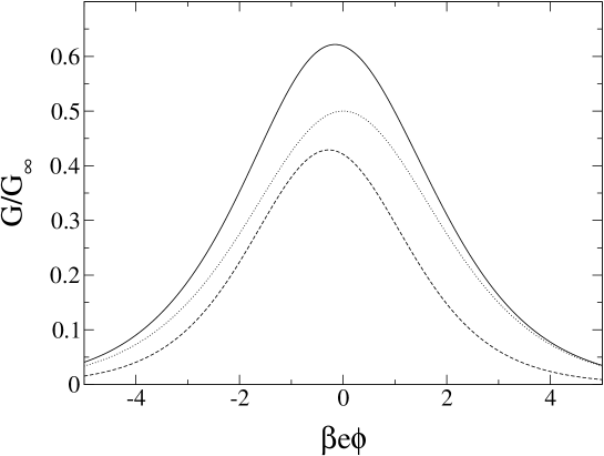
and is symmetric with respect to this value: $G(\phi-\phi_{LT})=G(\phi_{LT}-\phi)$. The exact line shape of the conductance peak, Eq. (62), at $T/\delta E=0.4$ and two limiting cases conductance peaks, Eqs. (63) and (64), plotted out of their validity region at $T/\delta E=0.4$ are shown in Fig. 11. As in the spinless case, the exact conductance peak is higher than both of the limiting cases peaks.

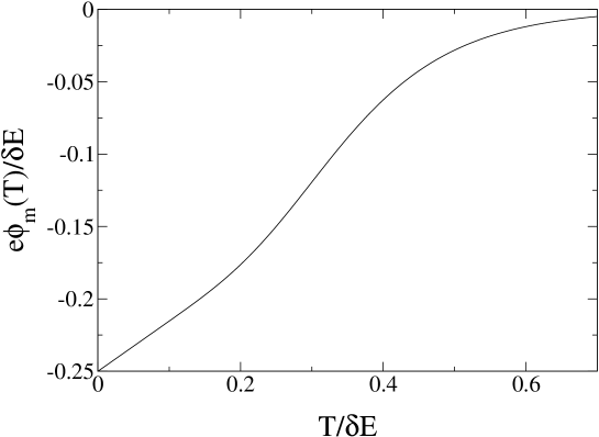
The position of the peak’s maximum, $\phi_{m}=\phi_{m}(T)$, is shifted to the left from its high temperature limit, $\phi_{CL}\equiv\phi_{m}(T\gg\delta E)=0$. It is determined by the equation for $\phi_{m}$: $G^{\prime}(\phi_{m})=0$, where $G(\phi)$ is given by Eq. (62). The dimensionless position of the peak’s maximum, $e\phi_{m}(T)/\delta E$, as a function of the temperature, $T/\delta E$, is numerically plotted in Fig. 12.

Figure 12: Temperature dependence of the dimensionless peak’s maximum position, $e\phi_{m}(T)/\delta E$. In the low temperature limit: $e\phi_{m}(0)/\delta E=-1/4$ according to Eq. (65).

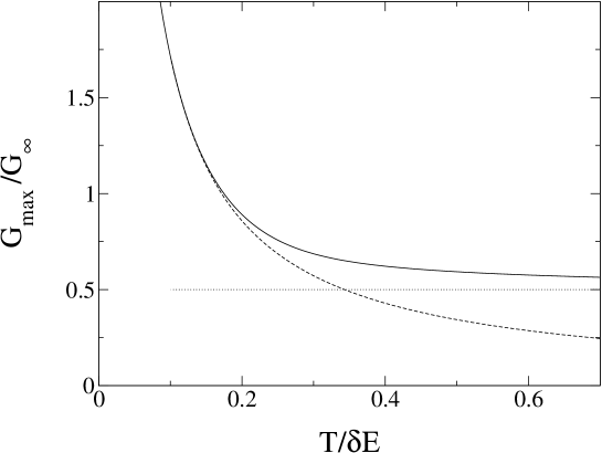
The conductance peak height is $G_{max}=G(\phi_{m})$. In the limiting cases:

$$\frac{G_{max}}{G_{\infty}}=\frac{G(\phi_{m})}{G_{\infty}}=\left\{\begin{array}[]{l}1/2,~{}~{}T\gg\delta E\\ (3-2\sqrt{2})\delta,~{}~{}\delta E\gg T\gg\Gamma_{i}\end{array}\right..$$ (66)

Peak’s height as a function of the temperature, $T/\delta E$, can be plotted numerically, Fig. 13.

Figure 13: Height of the conductance peak, $G_{max}/G_{\infty}$, as a function of the temperature, $T/\delta E$. Dotted and dashed curves correspond to two limiting cases peak heights, Eq. (66).

7 Conclusions

We have studied Coulomb blockade oscillations of the linear conductance through a quantum dot weakly coupled to the leads via multichannel tunnel junctions in the sequential tunneling approximation. To obtain analytical results we have assumed that the energy levels in the dot are equally spaced. The electron-electron interaction in a quantum dot has been described by the constant interaction model; though, thermal excitations with all possible spins have been taken into account.

The linear conductance in the spinless case is given by Eq. (22). It is valid at arbitrary values of $E_{C}$, $\delta E$ and $T$. The line shape of an individual conductance peak at arbitrary ratio $\delta=\delta E/T$ is given by Eq. (26). Exact conductance peak is higher than both of the limiting cases peaks at any gate voltage as is illustrated in Fig 5. An analytical expression for the height of the conductance peak at any ratio $\delta$ is obtained, Eq. (29).

In Section 5 we applied the spinless case theory result to the problem of the transport via a dot in the quantum Hall regime. Energy levels in a dot in this case are equidistant with the spacing given by Eq. (35).

Linear conductance in the case of spin-$\frac{1}{2}$ electrons at arbitrary values of $E_{C}$, $\delta E$, and $T$ is given by Eq. (58). In particular, this equation allows one to plot the conductance oscillations in the regime when the charging energy, level spacing in the dot, and the temperature are all of the same order, Fig. 9. We find that the period of Coulomb blockade oscillations is doubled compared to the model with a continuous electronic spectrum in the dot. Equation (58) is the main result of the chapter.

We also find that conductance in the odd valley is larger than that in the even one at any temperature, Fig. 10. The difference between conductances has the largest value at $T\approx 0.3~{}\delta E$ (at $\delta E=E_{C}$). The sign of the difference is the same as for the quantum dot in the Kondo regime [9]. Kondo effect takes place at very low temperatures, $T\lesssim T_{K}\ll T_{in}$, where $T_{K}$ is the Kondo temperature, and leads to the logarithmic enhancement of the conductance in the odd valleys [12]. Our consideration shows that even-odd asymmetry exists at much higher temperatures.

Line shape of the conductance peak is given by Eq. (62). As in the spinless case, the conductance peak is higher than both of the limiting cases peaks at any gate voltage, Fig 11. As we increase the temperature peaks’ maximums shift and become more equidistant, Fig 12. The peak’s height as a function of the temperature is calculated numerically and plotted in Fig. 13.

Though we have found physical system which has equidistant energy levels in the spinless case, see Section 5, we are not aware of any such system in the spin-$\frac{1}{2}$ case. In the case of a chaotic quantum dot Wigner-Dyson model gives a fairly good approximation for the distribution of the energy levels of the dot. If we had assumed Wigner-Dyson distribution of the quantum dot’s energy levels then we would have had to give up the hope of finding a solution. It goes back to the very difficult problem of finding occupation numbers of the dot’s energy levels in the canonical ensemble. The only way to solve it is to assume that energy levels in the quantum dot are equally spaced. Then one can use the bosonization technique to find the occupation numbers. Assumption of the equidistant energy levels is in line with the level repulsion property of the Wigner-Dyson distribution. Therefore, the analytical consideration of this reasonably simplified model, in our opinion, is a significant step forward in the solution of the general problem.

Though we do not expect our quantitative results to precisely describe a quantum dot with random energy levels, they certainly give correct order of magnitude for the conductance oscillations and their generic features.

Chapter 2 Coulomb Blockade Peak Spacings: Interplay of Spin and Dot-Lead Coupling

1 Overview

For Coulomb blockade peaks in the linear conductance of a quantum dot, we study the correction to the spacing between the peaks due to dot-lead coupling. This coupling can affect measurements in which Coulomb blockade phenomena are used as a tool to probe the energy level structure of quantum dots. The electron-electron interactions in the quantum dot are described by the constant exchange and interaction (CEI) model while the single-particle properties are described by random matrix theory. We find analytic expressions for both the average and rms mesoscopic fluctuation of the correction. For a realistic value of the exchange interaction constant $J_{\rm s}$, the ensemble average correction to the peak spacing is two to three times smaller than that at $J_{\rm s}\!=\!0$. As a function of $J_{\rm s}$, the average correction to the peak spacing for an even valley decreases monotonically, nonetheless staying positive. The rms fluctuation is of the same order as the average and weakly depends on $J_{\rm s}$. For a small fraction of quantum dots in the ensemble, therefore, the correction to the peak spacing for the even valley is negative. The correction to the spacing in the odd valleys is opposite in sign to that in the even valleys and equal in magnitude. These results are robust with respect to choice of the random matrix ensemble or change in parameters such as charging energy, mean level spacing, or temperature.

The work in this chapter was done in collaboration with Harold U. Baranger.

2 Introduction

Progress in nanoscale fabrication techniques has made possible not only the creation of more sophisticated devices but also greater control over their properties. Electron systems confined to small regions – quantum dots (QD) – and especially their transport properties have been studied extensively for the last decade [5, 11]. One of the most popular devices is a lateral quantum dot, formed by depleting the two-dimensional electron gas (2DEG) at the interface of a semiconductor heterostructure. By appropriately tuning negative potentials on the metal surface gates, one can control the QD size, the number of electrons $n$ it contains, as well as the tunnel barrier heights between the QD and the large 2DEG regions, which act as leads. Applying bias voltage $V$ between these leads allows one to study transport properties of a single electron transistor (SET), Fig. 1(a) [5].

We study properties of the conductance $G$ through a QD in the linear response regime. We assume that the dot is weakly coupled to the leads: $G_{L,R}\!\ll\!e^{2}/h$, where $G_{L,R}$ are the conductances of the dot-lead tunnel barriers, $e\!>\!0$ is the elementary charge, and $h$ is Planck’s constant.

To tunnel onto the quantum dot, an electron in the left lead has to overcome a charging energy $E_{C}\!=\!e^{2}/2C$, where $C$ is the capacitance of the QD, a phenomenon called the Coulomb blockade. However, if we apply voltage $V_{g}$ to an additional back-gate capacitively coupled to the QD, see Fig. 1(a), the Coulomb blockade can be lifted. Indeed, by changing $V_{g}$ one can change the electrostatics so that energies of the quantum dot with $n$ and $n+1$ electrons become equal, and so an electron can freely jump from the left lead onto the QD and then out to the right lead. Thus, a current event has occurred, and a peak in the conductance corresponding to that back-gate voltage, $V_{g,n+\frac{1}{2}}$, is observed. By sweeping the back-gate voltage, a series of peaks is observed, Fig. 1(b).

Figure 1: (a) Scheme of the Coulomb blockade setup; (b) Oscillations of the SET linear conductance $G$ as the back-gate voltage $V_{g}$ is changed. “Even” (“odd”) corresponds to an even (odd) number of electrons in the valley. Arrows show average shifts in the positions of the peaks’ maxima due to the finite dot-lead couplings.

In this chapter we calculate the correction to the spacing between Coulomb blockade peaks due to finite dot-lead tunnel coupling. In recent years, low-temperature Coulomb blockade experiments have been repeatedly used to probe the energy level structure of quantum dots [5, 11, 10]. The dot-lead tunnel coupling discussed here may influence such a measurement – the presence of leads may change what one sees – and so an understanding of coupling effects is needed. One dramatic consequence is the Kondo effect in quantum dots [8, 37, 9]. Here we assume that $T\!\gg\!T_{K}$, where $T_{K}$ is the Kondo temperature, and, therefore, do not consider Kondo physics, focusing instead on less dramatic effects that, however, survive to higher temperature.

We study an ensemble of chaotic ballistic (or chaotic disordered) quantum dots with large dimensionless conductance, $g\!\gg\!1$. The dimensionless conductance is defined as the ratio of the Thouless energy $E_{T}$ to the mean level spacing $\Delta$: $g\!\equiv\!E_{T}/\Delta$ [10]. For isolated quantum dots with large dimensionless conductance, the distribution of $g$ energy levels $\{\varepsilon_{k}\}$ near the Fermi level and the corresponding wave functions $\{\psi_{k}({\bf r})\}$ can be approximated by random matrix theory (RMT) [38, 10, 18]. As will be evident from what follows, the leading contribution to the results obtained here comes from $\xi\!\equiv\!2E_{C}/\Delta$ energy levels near the Fermi level; thus, if $E_{C}\lesssim E_{T}$ the statistics of these $\xi$ levels can be described by RMT. We furthermore neglect the spin-orbit interaction and, therefore, consider only the Gaussian orthogonal (GOE) and Gaussian unitary (GUE) ensembles of random matrices.

The microscopic theory of electron-electron interactions in a quantum dot with large dimensionless conductance brings about a remarkable result [19, 12]. To leading order, the interaction Hamiltonian depends only on the squares of the following two operators: (i) the total electron number operator $\hat{n}=\sum c_{k\sigma}^{\dagger}c_{k\sigma}$ where $\left\{c_{k\sigma}\right\}$ are the electron annihilation operators and $\sigma$ labels spin, and (ii) the total spin operator ${\hat{\bf S}}=\frac{1}{2}\sum c_{k\sigma_{1}}^{\dagger}\left<\sigma_{1}\right|{\hat{\bf\sigma}}\left|\sigma_{2}\right>c_{k\sigma_{2}}$ where $\left\{{\hat{\sigma}_{i}}\right\}$ are the Pauli matrices. The leading order part of the Hamiltonian reads [19, 12]

$$H_{\rm int}=E_{C}\,\hat{n}^{2}-J_{\rm s}\,{\hat{\bf S}}^{2}$$ (1)

where $E_{C}$ is the redefined value of the charging energy [19, 7] and $J_{\rm s}\!>\!0$ is the exchange interaction constant. Higher order corrections are of order $\Delta/g$ [19, 12, 20, 7]. The coupling constants in (1) are invariant with respect to different realizations of the quantum dot potential. This “universal” Hamiltonian is also invariant under arbitrary rotation of the basis and, therefore, compatible with RMT. In principal, the operator of interactions in the Cooper channel can appear in the “universal” Hamiltonian for the GOE case. However, if the quantum dot is in the normal state at $T\!=\!0$, then the corresponding coupling constant is positive and is renormalized to a very small value [19, 39]. The “universal” part of the Hamiltonian given by Eq. (1) is called the constant exchange and interaction (CEI) model [20, 7].

The total Hamiltonian of the quantum dot in the $g\!\to\!\infty$ limit thus has two parts, the single-particle RMT Hamiltonian and the CEI model describing the interactions. The capacitive QD-backgate coupling generates an additional term which is linear in the number of electrons:

$$H_{\rm dot}=\sum_{k\sigma}\varepsilon_{k}\,c_{k\sigma}^{\dagger}c_{k\sigma}+E_{C}\left(\hat{n}-{\mathcal{N}}\right)^{2}-J_{\rm s}\,{\hat{\bf S}}^{2}$$ (2)

where ${\mathcal{N}}\!=\!C_{g}V_{g}/e$ is the dimensionless back-gate voltage and $C_{g}$ is the QD-backgate capacitance.

The CEI model contains an additional exchange interaction term as compared to the conventional constant interaction model (CI model) [40, 41, 5]. Exchange is important as $J_{\rm s}$ is of the same order as $\Delta$, the mean single-particle level spacing. Indeed, in the realistic case of a 2DEG in a GaAs/AlGaAs heterostructure with gas parameter $r_{s}\!=\!1.5$, the static random phase approximation gives $J_{\rm s}\!\approx\!0.31\Delta$ [42]. Therefore, as we sweep the back-gate voltage, adding electrons to the quantum dot, the conventional up-down filling sequence may be violated [21, 22]. Indeed, energy level spacings do fluctuate: If for an even number of electrons $n$ in the QD the corresponding spacing, $\varepsilon_{\frac{n}{2}+1}-\varepsilon_{\frac{n}{2}}$, is less than $2J_{\rm s}$, then it becomes energetically favorable to promote an electron to the next orbital instead of putting it in the same one; thus, a triplet state ($S\!=\!1$) is formed. Higher spin states are possible as well. For $r_{s}\!=\!1.5$ the probability of forming a higher spin ground state is $P_{1}(S\!>\!0)\approx 0.26$ and $P_{2}(S\!>\!0)\approx 0.19$ for the GOE and GUE, respectively. The lower the electron density in the QD, the larger $r_{s}$ and, consequently, the larger the exchange interaction constant $J_{\rm s}$.

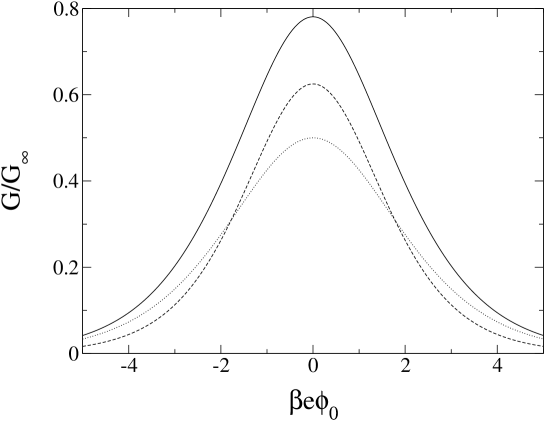
The back-gate voltage corresponding to the conductance peak maximum ${\mathcal{N}}_{n-\frac{1}{2}}$ is found by equating the energy for $n\!-\!1$ electrons in the dot with that for $n$ electrons:

$$E_{n-1}({\mathcal{N}}_{n-\frac{1}{2}})=E_{n}({\mathcal{N}}_{n-\frac{1}{2}})\;.$$ (3)

As we are interested in the effect of dot-lead coupling on these peak positions, it is natural to expand the energies perturbatively in this coupling: $E=E^{(0)}+E^{(2)}+\dots\,\,$. One possible virtual process contributing to $E^{(2)}$ is shown in Fig. 2. Electron occupations of the QD “to the left” and “to the right” of the conductance peak [see Fig. 1(b)] are different; hence, the corrections $E^{(2)}$ to the energies are different. Therefore, the position of the peak maximum acquires corrections as well, ${\mathcal{N}}={\mathcal{N}}^{(0)}+{\mathcal{N}}^{(2)}+\dots\,\,$, as does the spacing between two adjacent peaks.

Figure 2: One example of the virtual processes contributing to $E^{(2)}$. This virtual process corresponds to an electron tunneling out of the quantum dot into the left lead and then tunneling back into the same level in the QD.

This physical scenario has been considered by Kaminski and Glazman with the interactions treated in the CI model, i.e. neglecting exchange [43]. The ensemble averaged change in the spacing and its rms due to mesoscopic fluctuations were calculated. On average, “even” spacings (that is, spacings corresponding to an even number of electrons in the valley) increase, while “odd” spacings decrease (by the same amount) [43]:

$$2E_{C}~{}\overline{{\mathcal{U}}_{n}^{(2)}(J_{\rm s}\!=\!0)}=\Delta\,\frac{g_{L}+g_{R}}{2\pi^{2}}\,\ln\frac{2E_{C}}{T},$$ (4)

where ${\mathcal{U}}$ is the dimensionless spacing normalized by $2E_{C}$ and $g_{L,R}\!=\!G_{L,R}/(2e^{2}/h)$ are the dimensionless dot-lead conductances.

In this chapter we calculate the same quantities but with the electron-electron interactions in the QD described by the more realistic CEI model. We find that the average change in the spacing between conductance peaks is significantly less than that predicted by the CI model. However, the fluctuations are of the same order. In contrast to the CI result [43], for large enough $J_{\rm s}$, we find that “even” spacings do not necessarily increase (likewise, “odd” spacings do not necessarily decrease).

The chapter is organized as follows. In Section 3 we write down the total Hamiltonian of the system and find the condition for the tunneling Hamiltonian to be considered as a perturbation. In Section 4 we describe the approach and make symmetry remarks. In Section 5 we perform a detailed calculation of the correction to the spacing between Coulomb blockade peaks for the $\frac{1}{2}\to 1\to\frac{1}{2}$ spin sequence. In Section 6 we find the ensemble averaged correction to the peak spacing. The rms of the fluctuations of the correction to the peak spacing is calculated in Section 7. In Section 8 we summarize our findings and discuss their relevance to the available experimental data [44, 45].

3 The Hamiltonian

The Hamiltonian of the system in Fig. 1(a) consists of the QD Hamiltonian [Eq. (2)], the leads Hamiltonian, and the tunneling Hamiltonian accounting for the dot-lead coupling:

$$H=H_{\rm dot}+H_{\rm leads}+H_{\rm tun}.$$ (5)

The leads Hamiltonian can be written as follows

$$H_{\rm leads}=\sum_{{\bf p}\sigma}\varepsilon_{{\bf p}}c_{{\bf p}\sigma}^{\dagger}c_{{\bf p}\sigma}+\sum_{{\bf q}\sigma}\varepsilon_{{\bf q}}c_{{\bf q}\sigma}^{\dagger}c_{{\bf q}\sigma},$$ (6)

where $\{\varepsilon_{\bf p}\}$ and $\{\varepsilon_{\bf q}\}$ are the one-particle energies in the left and right leads, respectively, measured with respect to the chemical potential (see Fig. 2). We assume that the leads are large; therefore we (i) neglect electron-electron interactions in the leads and (ii) assume a continuum of states in each lead. The tunneling Hamiltonian is [46]

$$H_{\rm tun}=\sum_{k{\bf p}\sigma}(t_{k{\bf p}}c_{k\sigma}^{\dagger}c_{{\bf p}\sigma}+{\rm h.c.})+\sum_{k{\bf q}\sigma}(t_{k{\bf q}}c_{k\sigma}^{\dagger}c_{{\bf q}\sigma}+{\rm h.c.}),$$ (7)

where $\{t_{k{\bf p}}\}$ and $\{t_{k{\bf q}}\}$ are the tunneling matrix elements.

We assume that $T\!\ll\!\Delta$ and, therefore, neglect excited states of the QD concentrating on ground state properties only. We also assume that the QD is weakly coupled to the leads, treating the tunneling Hamiltonian as a perturbation. Corrections to the position of the peak maximum can be expressed in terms of corrections to the ground state energies of the QD via Eq. (3). The perturbation series for these corrections contains only even powers as $H_{\rm tun}$ is off-diagonal in the eigenbasis of $H_{0}$. The $2m^{\rm th}$ correction to the position of the peak is roughly

$$2E_{C}~{}\overline{{\mathcal{N}}^{(2m)}}\approx\Delta\,\frac{g_{L}+g_{R}}{4\pi^{2}}\,\ln\frac{2E_{C}}{T}\left(\frac{g_{L}+g_{R}}{4\pi^{2}}\,\ln\frac{2E_{C}}{\Delta}\,\ln\frac{2E_{C}}{T}\right)^{m-1}.$$ (8)

Thus, finite-order perturbation theory is applicable if [43]

$$\frac{g_{L}+g_{R}}{4\pi^{2}}~{}\ln\left(\frac{2E_{C}}{\Delta}\right)\ln\left(\frac{2E_{C}}{T}\right)\ll 1.$$ (9)

To loosen this restriction one should deploy a renormalization group technique which, however, is beyond the scope of this chapter [43, 47, 48, 49].

4 Plan of the Calculation

As the exchange interaction constant $J_{\rm s}$ becomes larger, more values of the QD spin $S$ become accessible. The structure of the corrections to the ground state energies depends on the total QD spin $S$, and this structure becomes very complicated for large values of the spin $S$. Fortunately, for the realistic case $r_{s}=1.5$, the probability of spin values higher than $\frac{1}{2}$ in an “odd” valley is small: $P_{2}(S\!>\!\frac{1}{2})\approx 0.01$ for the GUE. Hence, we can safely assume that in the “odd” valley the spin is always equal to $\frac{1}{2}$. In the “even” valley, one has to allow both $S\!=\!0$ and $S\!=\!1$ states.

The structure of the expression for the spacing between peaks depends on the allowed spin sequences. For an “even” valley there are only two possible spin sequences:

$${\textstyle\frac{1}{2}}\to 0\to{\textstyle\frac{1}{2}}~{}~{}~{}~{}\mbox{and}~{}~{}~{}~{}{\textstyle\frac{1}{2}}\to 1\to{\textstyle\frac{1}{2}}$$ (10)

where the number in the middle is the spin in the “even” valley, while the numbers to the left and right are spin values in the adjacent valleys, Fig. 1(b). For an “odd” valley there are four possibilities:

$$0\to{\textstyle\frac{1}{2}}\to 0,~{}~{}~{}~{}0\to{\textstyle\frac{1}{2}}\to 1,$$

$$1\to{\textstyle\frac{1}{2}}\to 0,~{}~{}~{}~{}\mbox{and}~{}~{}~{}~{}1\to{\textstyle\frac{1}{2}}\to 1\;.$$ (11)

To obtain correct expressions for the average spacing between peaks, one should weight these sequences with the appropriate probability of occurrence.

Before proceeding with the calculations, we note several general properties. First, ensemble averaged corrections to the “odd” and “even” spacings are of the same magnitude and opposite sign, Fig. 1(b). Second, the mesoscopic fluctuations of both corrections are equal. Indeed, the shift in position of an “even-odd” ($n\to n\!+\!1$) peak maximum, Fig. 1(b), is determined by the interplay between the $0\!\to\!\frac{1}{2}$ and $1\!\to\!\frac{1}{2}$ spin sequences. Likewise, the shift of the “odd-even” ($n\!-\!1\to n$) peak is determined by the $\frac{1}{2}\!\to\!0$ and $\frac{1}{2}\!\to\!1$ spin sequences. Now if we sweep the back-gate voltage in the opposite direction and write the same peak as $n\to n\!-\!1$, then the corresponding spin sequences are exactly the same as they were in the first case: $0\!\to\!\frac{1}{2}$ and $1\!\to\!\frac{1}{2}$. From this symmetry argument one can conclude that (i) the ensemble averaged shifts of the “even-odd” and “odd-even” peaks are of the same magnitude and in the opposite directions [43] and (ii) the mesoscopic fluctuations of both shifts are equal.

Thus, to simplify the calculations we study only the “even” spacing case. This corresponds to the two spin sequences given in Eq. (10). First, we calculate corrections to the spacing between peaks for both spin sequences. A complete calculation for the doublet-triplet-doublet spin sequence is in the next section. Second, we elaborate on how to put these spacings together in the final expression for an “even” spacing. Finally, we calculate GOE and GUE ensemble averaged corrections to the spacing and the rms fluctuations.

5 Doublet-Triplet-Doublet Spin Sequence: Calculation of the Spacing Between Peaks

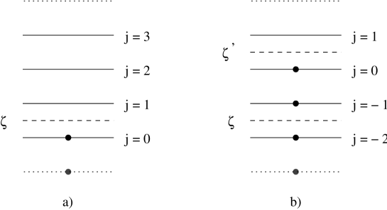
Let us find the correction to the spacing between peaks for a doublet-triplet-doublet spin sequence. The corresponding electron occupation of the quantum dot in three consecutive valleys with $n\!-\!1$, $n$, and $n\!+\!1$ electrons is shown in Fig. 3.

Figure 3: Occupation of the QD levels in the ground state in three consecutive valleys with total electron number $n-1$, $n$, and $n+1$, respectively. A doublet-triplet-doublet spin sequence is shown. The variables $x$, $(x_{1},x_{2},\dots)$, and $(y_{1},y_{2},\dots)$ denote the energy level spacings in the QD normalized by mean level spacing $\Delta$. For example, $x\!=\!\left(\varepsilon_{\frac{n}{2}+1}-\varepsilon_{\frac{n}{2}}\right)/\Delta$.

For the isolated QD the position of the $n\!-\!1\to n$ conductance peak maximum is determined by

$$E^{(0)}_{n-1,S=\frac{1}{2}}\big{(}{\mathcal{N}}^{(0)}_{n-\frac{1}{2}}\big{)}=E^{(0)}_{n,S=1}\big{(}{\mathcal{N}}^{(0)}_{n-\frac{1}{2}}\big{)}$$ (12)

where $E_{n-1,S=\frac{1}{2}}^{(0)}$ and $E_{n,S=1}^{(0)}$ are the ground state energies of dot Hamiltonian [Eq. (2)]. The corrections due to dot-lead tunneling are different for the doublet and triplet states. The resultant shift in peak position is given by [43]

$${\mathcal{N}}^{(2)}_{n-\frac{1}{2}}=\frac{1}{2E_{C}}\left[E^{(2)}_{n,S=1}\big{(}{\mathcal{N}}^{(0)}_{n-\frac{1}{2}}\big{)}-E^{(2)}_{n-1,S=\frac{1}{2}}\big{(}{\mathcal{N}}^{(0)}_{n-\frac{1}{2}}\big{)}\right]\;.$$ (13)

Note that for the second-order correction to the position, the ground state energies are taken at the gate voltage obtained in the zeroth-order calculation, Eq. (12).

Analogous equations hold for the $n\to n\!+\!1$ conductance peak. The spacing between these two conductance peaks is then defined as

$${\mathcal{U}}_{n,S=1}={\mathcal{N}}_{n+\frac{1}{2}}\big{(}1\to{\textstyle\frac{1}{2}}\big{)}-{\mathcal{N}}_{n-\frac{1}{2}}\big{(}{\textstyle\frac{1}{2}}\to 1\big{)}.$$ (14)

1 Zeroth Order: Isolated Quantum Dot

For the doublet-triplet $n\!-\!1\to n$ sequence Eq. (12) gives

$${\mathcal{N}}^{(0)}_{n-\frac{1}{2}}\big{(}{\textstyle\frac{1}{2}}\to 1\big{)}=n-\frac{1}{2}+\frac{1}{2E_{C}}\left(\varepsilon_{\frac{n}{2}+1}-\frac{5}{4}J_{\rm s}-\frac{T}{2}\ln\frac{3}{2}\right)$$ (15)

where the last temperature dependent term is the entropic correction to the condition of equal energies [31]. For the position of the $n\to n\!+\!1$ peak maximum we obtain

$${\mathcal{N}}^{(0)}_{n+\frac{1}{2}}\big{(}1\to{\textstyle\frac{1}{2}}\big{)}=n+\frac{1}{2}+\frac{1}{2E_{C}}\left(\varepsilon_{\frac{n}{2}}+\frac{5}{4}J_{\rm s}+\frac{T}{2}\ln\frac{3}{2}\right).$$ (16)

Thus the spacing between peaks in zeroth order is

$${\mathcal{U}}^{(0)}_{n,S=1}(x)=1+\frac{5j-2x}{2\xi}+\frac{T}{2E_{C}}\ln\frac{3}{2},$$ (17)

where $j\!=\!J_{\rm s}/\Delta$ and $x\!=\!\left(\varepsilon_{\frac{n}{2}+1}-\varepsilon_{\frac{n}{2}}\right)/\Delta$ (see Fig. 3). Similarly, for the doublet-singlet-doublet spin sequence the spacing is

$${\mathcal{U}}^{(0)}_{n,S=0}(x)=1+\frac{2x-3j}{2\xi}-\frac{T}{2E_{C}}\ln 2.$$ (18)

Note that in both cases ${\mathcal{U}}_{n}^{(0)}$ depends only on the spacing $x$.

2 Second Order: Contribution From Virtual Processes

Figure 4: Six distinct types of the virtual processes contribute to the ground state energy correction for the QD in the triplet state. Only tunneling processes in (or out of) the left lead are shown. In the first four cases spin of the dot in the virtual state ${\mathcal{S}}$ has a definite value. In the last two cases (e) and (f) QD spin in the virtual state has two allowed values: ${\mathcal{S}}=\frac{1}{2}$ and ${\mathcal{S}}=\frac{3}{2}$ with the probabilities $w_{\mathcal{S}}$ given by Eq. (21). Electron structure of the virtual state corresponding to two allowed values of ${\mathcal{S}}$ is circled by dashed line in panel (e).

Let us consider in detail the second-order correction to the ground state energy of the triplet for subsequent use in (13):

$$E^{(2)}_{n,S=1}\left({\mathcal{N}}\right)={\sum_{m}}^{\prime}\frac{\left|\left<\psi^{(0)}_{m}\left|H_{\rm tun}\right|\psi^{(0)}_{n,S=1}\right>\right|^{2}}{E^{(0)}_{n,S=1}\left({\mathcal{N}}\right)-E^{(0)}_{m}\left({\mathcal{N}}\right)},$$ (19)

where the sum is over all possible virtual states. $E^{(0)}$ and $\left|\psi^{(0)}\right>$ are the eigenvalues and eigenvectors of $H_{\rm dot}$, Eq. (2).

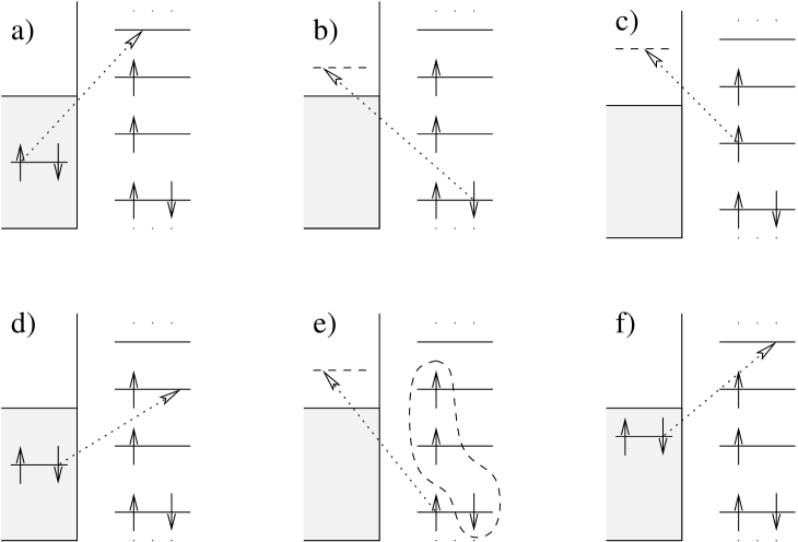
Different terms in Eq. (19) have different structure depending on the type of virtual state involved; six possibilities are shown in Fig. 4. To take into account all virtual processes, we sum over all energy levels in the QD and integrate over states in each lead. To simplify the calculation even further, we assume (just for a moment) that $T\!=\!0$ so that the Fermi distribution in the leads is a step function. Later we will see how $T$ reappears as a lower cutoff within a logarithm.

Following the order of terms in Fig. 4, the second-order correction to the triplet ground state energy is

$$E^{(2)}_{n,S=1}({\mathcal{N}})= - \sum^{\infty}_{k=\frac{n}{2}+2}\sum_{{\bf p}}\frac{\theta(-\varepsilon_{\bf p})\left|t_{k{\bf p}}\right|^{2}}{\left(\varepsilon_{k}-\varepsilon_{\bf p}\right)+2E_{C}(n+\frac{1}{2}-{\mathcal{N}})-\frac{7}{4}J_{\rm s}}$$ (20)

$$- \sum_{k=1}^{\frac{n}{2}-1}\sum_{{\bf p}}\frac{\theta(\varepsilon_{\bf p})\left|t_{k{\bf p}}\right|^{2}}{\left(\varepsilon_{\bf p}-\varepsilon_{k}\right)-2E_{C}(n-\frac{1}{2}-{\mathcal{N}})-\frac{7}{4}J_{\rm s}}$$

$$- \sum^{\frac{n}{2}+1}_{k=\frac{n}{2}}\sum_{{\bf p}}\frac{\theta(\varepsilon_{\bf p})\left|t_{k{\bf p}}\right|^{2}}{\left(\varepsilon_{\bf p}-\varepsilon_{k}\right)-2E_{C}(n-\frac{1}{2}-{\mathcal{N}})+\frac{5}{4}J_{\rm s}}$$

$$- \sum_{k=\frac{n}{2}}^{\frac{n}{2}+1}\sum_{{\bf p}}\frac{\theta(-\varepsilon_{\bf p})\left|t_{k{\bf p}}\right|^{2}}{\left(\varepsilon_{k}-\varepsilon_{\bf p}\right)+2E_{C}(n+\frac{1}{2}-{\mathcal{N}})+\frac{5}{4}J_{\rm s}}$$

$$- \sum_{{\mathcal{S}}=\frac{1}{2},\frac{3}{2}}w_{\mathcal{S}}\left[\sum^{\frac{n}{2}-1}_{k=1}\sum_{{\bf p}}\frac{\theta(\varepsilon_{\bf p})\left|t_{k{\bf p}}\right|^{2}}{\left(\varepsilon_{\bf p}-\varepsilon_{k}\right)-2E_{C}(n-\frac{1}{2}-{\mathcal{N}})+f_{\mathcal{S}}J_{\rm s}}\right.$$

$$+ \left.\sum_{k=\frac{n}{2}+2}^{\infty}\sum_{{\bf p}}\frac{\theta(-\varepsilon_{\bf p})\left|t_{k{\bf p}}\right|^{2}}{\left(\varepsilon_{k}-\varepsilon_{\bf p}\right)+2E_{C}(n+\frac{1}{2}-{\mathcal{N}})+f_{\mathcal{S}}J_{\rm s}}\right]$$

$$+ \left\{\mbox{similar terms for the right lead:}~{}{\bf p}\to{\bf q}\right\},$$

where ${\mathcal{S}}$ is the spin of the QD in the virtual state. One can easily find ${\mathcal{S}}$ for the first four processes, Figs. 4(a)-(d), and so calculate the denominators for the first four terms in (20): the values are $\frac{3}{2}$, $\frac{3}{2}$, $\frac{1}{2}$, and $\frac{1}{2}$, respectively. In the last two cases, Figs. 4(e)-(f), the QD spin in the virtual state can take two values, ${\mathcal{S}}=\frac{1}{2}$ or $\frac{3}{2}$; it does so with the following probabilities

$$w_{\frac{1}{2}}={\textstyle\frac{2}{3}}~{}~{}~{}~{}\mbox{and}~{}~{}~{}~{}w_{\frac{3}{2}}={\textstyle\frac{1}{3}}\;.$$ (21)

The corresponding contributions to the energy correction must be weighted accordingly. In addition, the energy difference in the denominators depends on ${\mathcal{S}}$; to account for this dependence, we introduce an additional function

$$f_{\mathcal{S}}\equiv 2-{\mathcal{S}}\left({\mathcal{S}}+1\right),$$ (22)

appearing in the denominators of the fifth and sixth terms in (20).

Let us integrate over the continuous energy levels in the lead. The sum can be replaced by an integral, $\sum_{\bf p}\,\cdots~{}\longrightarrow\int d\varepsilon~{}\nu_{L}(\varepsilon)\,\cdots\;$, where $\nu_{L}$ is the density of states in the left lead. Taking the dot-lead contacts to be point-like, the tunneling matrix elements $\{t_{k{\bf p}}\}$ depend on the momentum in the lead ${\bf p}$ only weakly; hence, $t_{k{\bf p}}\approx t_{kL}$. In addition, as the leads are formed from 2DEG, their density of states is roughly independent of energy. We assume that it is constant in the energy band of $2E_{C}$ near the Fermi surface. Then the result of integrating over the energy spectrum in the lead (in schematic form) for the first term in Eq. (20) is

$$\sum_{\bf p}\frac{\theta(-\varepsilon_{\bf p})\left|t_{k{\bf p}}\right|^{2}}{\epsilon_{k}-\varepsilon_{\bf p}}~{}\longrightarrow~{}\nu_{L}\left|t_{kL}\right|^{2}\ln\left|\frac{\varepsilon}{\epsilon_{k}}\right|_{\varepsilon\to\infty}.$$ (23)

This expression diverges, but when we calculate an observable, e.g. the shift in the position of the peak maximum [Eq. (13)], we encounter the energy difference between corrections to the triplet and doublet states. The result for the shift is, therefore, finite:

$$\left.\left(\ln\left|\frac{\varepsilon}{\epsilon_{k}}\right|-\ln\left|\frac{\varepsilon}{\epsilon^{\prime}_{k}}\right|\right)\right|_{\varepsilon\to\infty}=\ln\left|\frac{\epsilon^{\prime}_{k}}{\epsilon_{k}}\right|.$$ (24)

In a similar fashion one can calculate the second-order correction to the ground state energy of the doublet. The difference of these energies at the gate voltage corresponding to the peak maximum in zeroth order [Eq. (15)], needed in Eq. (13), then follows. There is one resonant term, proportional to $\ln\left({2E_{C}}/{T}\right)$, in which the lower cutoff $T$ appears because of the entropic term in Eq. (15). Alternatively, $T$ would appear as the natural cutoff for the resonant term upon reintroduction of the Fermi-Dirac distribution for the occupation numbers in the leads.

For a point-like dot-lead contact, the tunneling matrix element is proportional to the value of the electron wave function in the QD at the point of contact: $t_{k\alpha}\propto\psi_{k}({\bf r}_{\alpha})$, where $\alpha=L$ or $R$. Here, we neglect the fluctuations of the electron wave function in the large lead. Thus, the following identity is valid

$$\nu_{\alpha}\left|t_{k\alpha}\right|^{2}=\frac{\Delta}{4\pi^{2}}~{}g_{\alpha}\frac{\left|\psi_{k}\left({\bf r}_{\alpha}\right)\right|^{2}}{\left<\left|\psi_{k}\left({\bf r}_{\alpha}\right)\right|^{2}\right>},$$ (25)

where the average in the denominator is taken over the statistical ensemble. Note that by taking the ensemble average of both sides of (25), one arrives at the standard golden rule expression for the dimensionless conductance.

In our calculations we take advantage of the fact that $J_{\rm s}\!<\!\Delta\!\ll\!E_{C}$ and neglect terms that are of order $1/\xi\!=\!\Delta/2E_{C}$. Sums like

$$-\frac{1}{2}\sum_{k=\frac{n}{2}+2}^{\infty}\ln\left(1+\frac{2J_{\rm s}}{\varepsilon_{k}-\varepsilon_{\frac{n}{2}+1}}\right)$$ (26)

are split using $\sum_{k=\frac{n}{2}+2}^{\infty}\cdots\!=\!\sum_{k=\frac{n}{2}+2}^{\frac{n}{2}+\xi+1}\cdots\!+\!\sum_{k=\frac{n}{2}+\xi+2}^{\infty}\cdots$, and so the last term, which is $O(1/\xi)$, is dropped. Likewise, expressions like

$$\frac{2}{3}\sum_{k=\frac{n}{2}+2}^{\infty}\ln\left(1+\frac{3}{2}~{}\frac{J_{\rm s}}{\varepsilon_{k}-\varepsilon_{\frac{n}{2}+1}+2E_{C}}\right)$$ (27)

are of order $O(1/\xi)$ and so neglected.

Thus, for the second order correction to the position of the peak maximum, we obtain

$${\mathcal{N}}^{(2)}_{n-\frac{1}{2}}\left(\frac{1}{2}\to 1\right)=\frac{1}{4\pi^{2}\xi}\sum_{\alpha=L,R}g_{\alpha}$$ (28)

$$\times \left[-2\sum_{k\neq\frac{n}{2},\frac{n}{2}+1}\mbox{sign}\left(\frac{n}{2}-k\right)\frac{\left|\psi_{k}\left({\bf r}_{\alpha}\right)\right|^{2}}{\left<\left|\psi_{k}\left({\bf r}_{\alpha}\right)\right|^{2}\right>}\ln\left(\frac{2E_{C}}{\left|\varepsilon_{\frac{n}{2}+1}-\varepsilon_{k}\right|}+1\right)\right.$$

$$- \left.\frac{\left|\psi_{\frac{n}{2}}\left({\bf r}_{\alpha}\right)\right|^{2}}{\left<\left|\psi_{\frac{n}{2}}\left({\bf r}_{\alpha}\right)\right|^{2}\right>}\ln\left(\frac{2J_{\rm s}}{\varepsilon_{\frac{n}{2}+1}-\varepsilon_{\frac{n}{2}}}-1\right)\right.+\left.\frac{1}{2}\frac{\left|\psi_{\frac{n}{2}+1}\left({\bf r}_{\alpha}\right)\right|^{2}}{\left<\left|\psi_{\frac{n}{2}+1}\left({\bf r}_{\alpha}\right)\right|^{2}\right>}\left(\ln\frac{E_{C}}{J_{\rm s}}+\ln\frac{2E_{C}}{T}\right)\right.$$

$$+ \left.\frac{4}{3}\sum_{k=\frac{n}{2}-\xi}^{\frac{n}{2}-1}\frac{\left|\psi_{k}\left({\bf r}_{\alpha}\right)\right|^{2}}{\left<\left|\psi_{k}\left({\bf r}_{\alpha}\right)\right|^{2}\right>}\ln\left|1-\frac{3J_{\rm s}}{\varepsilon_{\frac{n}{2}+1}-\varepsilon_{k}}\right|\right.$$

$$- \left.\frac{1}{2}\sum_{k=\frac{n}{2}+2}^{\frac{n}{2}+\xi}\frac{\left|\psi_{k}\left({\bf r}_{\alpha}\right)\right|^{2}}{\left<\left|\psi_{k}\left({\bf r}_{\alpha}\right)\right|^{2}\right>}\ln\left(1+\frac{2J_{\rm s}}{\varepsilon_{k}-\varepsilon_{\frac{n}{2}+1}}\right)+O\left(\frac{1}{\xi}\right)\right],$$

where $2J_{\rm s}>\varepsilon_{\frac{n}{2}+1}\!-\!\varepsilon_{\frac{n}{2}}>0$ because the total spin of the QD with $n$ electrons is equal to 1.

In a similar fashion one can find the shift in the position of the other peak maximum, ${\mathcal{N}}^{(2)}_{\frac{n}{2}+1}\left(1\to\frac{1}{2}\right)$. Then, according to (14), the difference of these two shifts yields the second-order correction to the spacing for the doublet-triplet-doublet spin sequence:

$${\mathcal{U}}_{n,S=1}^{(2)} = \frac{1}{4\pi^{2}\xi}\sum_{\alpha=L,R}g_{\alpha}\left\{2\sum_{k\neq\frac{n}{2},\frac{n}{2}+1}\mbox{sign}\left(\frac{n}{2}-k\right)\frac{\left|\psi_{k}\left({\bf r}_{\alpha}\right)\right|^{2}}{\left<\left|\psi_{k}\left({\bf r}_{\alpha}\right)\right|^{2}\right>}\right.$$ (29)

$$\times \left[\ln\left(\frac{2E_{C}}{\left|\varepsilon_{\frac{n}{2}+1}-\varepsilon_{k}\right|}+1\right)-\ln\left(\frac{2E_{C}}{\left|\varepsilon_{\frac{n}{2}}-\varepsilon_{k}\right|}+1\right)\right]$$

$$+ \left(\frac{\left|\psi_{\frac{n}{2}}\left({\bf r}_{\alpha}\right)\right|^{2}}{\left<\left|\psi_{\frac{n}{2}}\left({\bf r}_{\alpha}\right)\right|^{2}\right>}+\frac{\left|\psi_{\frac{n}{2}+1}\left({\bf r}_{\alpha}\right)\right|^{2}}{\left<\left|\psi_{\frac{n}{2}+1}\left({\bf r}_{\alpha}\right)\right|^{2}\right>}\right)$$

$$\times \left[\ln\left(\frac{2J_{\rm s}}{\varepsilon_{\frac{n}{2}+1}-\varepsilon_{\frac{n}{2}}}-1\right)-\frac{1}{2}\ln\frac{E_{C}}{J_{\rm s}}-\frac{1}{2}\ln\frac{2E_{C}}{T}\right]$$

$$+ \left.\sum_{k=\frac{n}{2}-\xi}^{\frac{n}{2}-1}\frac{\left|\psi_{k}\left({\bf r}_{\alpha}\right)\right|^{2}}{\left<\left|\psi_{k}\left({\bf r}_{\alpha}\right)\right|^{2}\right>}\left[\frac{1}{2}\ln\left(1+\frac{2J_{\rm s}}{\varepsilon_{\frac{n}{2}}-\varepsilon_{k}}\right)-\frac{4}{3}\ln\left|1-\frac{3J_{\rm s}}{\varepsilon_{\frac{n}{2}+1}-\varepsilon_{k}}\right|\right]\right.$$

$$+ \sum_{k=\frac{n}{2}+2}^{\frac{n}{2}+\xi}\frac{\left|\psi_{k}\left({\bf r}_{\alpha}\right)\right|^{2}}{\left<\left|\psi_{k}\left({\bf r}_{\alpha}\right)\right|^{2}\right>}\left[\frac{1}{2}\ln\left(1+\frac{2J_{\rm s}}{\varepsilon_{k}-\varepsilon_{\frac{n}{2}+1}}\right)-\frac{4}{3}\ln\left|1-\frac{3J_{\rm s}}{\varepsilon_{k}-\varepsilon_{\frac{n}{2}}}\right|\right]$$

$$+ \left.O\left(\frac{1}{\xi}\right)\right\}.$$

A potential complication is that the addition of two electrons to the quantum dot ($n\!-\!1\to n\to n\!+\!1$) may scramble the energy levels and wave functions of the QD [50, 51, 7]. Since the number of added electrons is small, we assume that the same realization of the Hamiltonian, Eq. (5), is valid in all three valleys [52, 53].

For the second-order correction to the spacing for the doublet-singlet-doublet spin sequence we similarly obtain

$${\mathcal{U}}_{n,S=0}^{(2)} = \frac{1}{4\pi^{2}\xi}\sum_{\alpha=L,R}g_{\alpha}\left\{-2\sum_{k\neq\frac{n}{2},\frac{n}{2}+1}\mbox{sign}\left(\frac{n}{2}-k\right)\frac{\left|\psi_{k}\left({\bf r}_{\alpha}\right)\right|^{2}}{\left<\left|\psi_{k}\left({\bf r}_{\alpha}\right)\right|^{2}\right>}\right.$$ (30)

$$\times \left[\ln\left(\frac{2E_{C}}{\left|\varepsilon_{\frac{n}{2}+1}-\varepsilon_{k}\right|}+1\right)-\ln\left(\frac{2E_{C}}{\left|\varepsilon_{\frac{n}{2}}-\varepsilon_{k}\right|}+1\right)\right]$$

$$+ \left(\frac{\left|\psi_{\frac{n}{2}}\left({\bf r}_{\alpha}\right)\right|^{2}}{\left<\left|\psi_{\frac{n}{2}}\left({\bf r}_{\alpha}\right)\right|^{2}\right>}+\frac{\left|\psi_{\frac{n}{2}+1}\left({\bf r}_{\alpha}\right)\right|^{2}}{\left<\left|\psi_{\frac{n}{2}+1}\left({\bf r}_{\alpha}\right)\right|^{2}\right>}\right)$$

$$\times \left[\frac{3}{2}\ln\left(1-\frac{2J_{\rm s}}{\varepsilon_{\frac{n}{2}+1}-\varepsilon_{\frac{n}{2}}}\right)-2\ln\left(\frac{2E_{C}}{\varepsilon_{\frac{n}{2}+1}-\varepsilon_{\frac{n}{2}}}+1\right)+\ln\frac{2E_{C}}{T}\right]$$

$$+ \frac{3}{2}\sum_{k=\frac{n}{2}-\xi}^{\frac{n}{2}-1}\frac{\left|\psi_{k}\left({\bf r}_{\alpha}\right)\right|^{2}}{\left<\left|\psi_{k}\left({\bf r}_{\alpha}\right)\right|^{2}\right>}\ln\left(1-\frac{2J_{\rm s}}{\varepsilon_{\frac{n}{2}+1}-\varepsilon_{k}}\right)$$

$$+ \left.\frac{3}{2}\sum_{k=\frac{n}{2}+2}^{\frac{n}{2}+\xi}\frac{\left|\psi_{k}\left({\bf r}_{\alpha}\right)\right|^{2}}{\left<\left|\psi_{k}\left({\bf r}_{\alpha}\right)\right|^{2}\right>}\ln\left(1-\frac{2J_{\rm s}}{\varepsilon_{k}-\varepsilon_{\frac{n}{2}}}\right)+O\left(\frac{1}{\xi}\right)\right\},$$

where $\varepsilon_{\frac{n}{2}+1}\!-\!\varepsilon_{\frac{n}{2}}>2J_{\rm s}\geq 0$ because the total spin of the QD with $n$ electrons is equal to $0$ in this case.

Unlike the zeroth-order spacings, the second-order corrections are functions of many energy level spacings as well as the wave functions at the dot-lead contact points: ${\mathcal{U}}_{n,S}^{(2)}={\mathcal{U}}_{n,S}^{(2)}(x,{\bf X},{\bf Y};\{Z_{k\alpha}\})$, where $x$, ${\bf X}=(x_{1},x_{2},\dots)$, and ${\bf Y}=(y_{1},y_{2},\dots)$ are the energy level spacings in the QD normalized by the mean level spacing $\Delta$ (see Fig. 3) and

$$Z_{k\alpha}\equiv\frac{\left|\psi_{k}\left({\bf r}_{\alpha}\right)\right|^{2}}{\left<\left|\psi_{k}\left({\bf r}_{\alpha}\right)\right|^{2}\right>}\;.$$ (31)

The expressions for ${\mathcal{U}}^{(2)}$ suggest that the main contribution to their fluctuation comes from the fluctuation of the energy level $x$ and the wave functions $\left\{\psi_{k}\left({\bf r}_{\alpha}\right)\right\}$. The other spacings, ${\bf X}$ and ${\bf Y}$, always appear within a logarithm; therefore, their contribution to the fluctuation of ${\mathcal{U}}^{(2)}$ is small. With good accuracy, one can replace these levels by their mean value

$${\mathcal{U}}_{n,S}^{(2)}\approx{\mathcal{U}}_{n,S}^{(2)}(x,{\bf 1},{\bf 1};\{Z_{k\alpha}\})\equiv{\mathcal{U}}_{n,S}^{(2)}(x;\{Z_{k\alpha}\})\;.$$ (32)

Converting to dimensionless units, we find that

$${\mathcal{U}}^{(2)}_{n,S}\left(x;\left\{Z_{k\alpha}\right\}\right)=\frac{1}{4\pi^{2}\xi}\sum_{\alpha=L,R}g_{\alpha}\Phi_{\alpha,S}\left(x;\left\{Z_{k\alpha}\right\}\right),$$ (33)

where

$$\Phi_{\alpha,S=0}\left(x;\left\{Z_{k\alpha}\right\}\right) = \left(Z_{\frac{n}{2},\alpha}+Z_{\frac{n}{2}+1,\alpha}\right)\left[-\ln\xi+\ln\delta+\frac{1}{2}\ln x+\frac{3}{2}\ln(x-2j)\right]$$ (34)

$$+ 2\sum_{l=1}^{\infty}\left(Z_{\frac{n}{2}-l,\alpha}+Z_{\frac{n}{2}+1+l,\alpha}\right)\left[\ln\left(1+\frac{x}{l}\right)-\ln\left(1+\frac{x}{\xi+l}\right)\right]$$

$$+ \frac{3}{2}\sum_{l=1}^{\xi}\left(Z_{\frac{n}{2}-l,\alpha}+Z_{\frac{n}{2}+1+l,\alpha}\right)\ln\left(1-\frac{2j}{x+l}\right)+O\left(1\right),$$

$$\Phi_{\alpha,S=1}\left(x;\left\{Z_{k\alpha}\right\}\right)=\left(Z_{\frac{n}{2},\alpha}+Z_{\frac{n}{2}+1,\alpha}\right)\left[-\ln\xi-\frac{1}{2}\ln\delta+\frac{1}{2}\ln 2j+\ln\left(\frac{2j}{x}-1\right)\right]$$ (35)

$$- 2\sum_{l=1}^{\infty}\left(Z_{\frac{n}{2}-l,\alpha}+Z_{\frac{n}{2}+1+l,\alpha}\right)\left[\ln\left(1+\frac{x}{l}\right)-\ln\left(1+\frac{x}{\xi+l}\right)\right]$$

$$+ \sum_{l=1}^{\xi}\left(Z_{\frac{n}{2}-l,\alpha}+Z_{\frac{n}{2}+1+l,\alpha}\right)\left[\frac{1}{2}\ln\left(1+\frac{2j}{l}\right)-\frac{4}{3}\ln\left|1-\frac{3j}{x+l}\right|\right]+O\left(1\right),$$

where $\delta=\Delta/T$. Here, the upper limit in two of the sums is infinity because the Fermi energy is the largest energy scale.

In summary, the total spacing is

$${\mathcal{U}}_{n,S}={\mathcal{U}}_{n,S}^{(0)}(x)+{\mathcal{U}}_{n,S}^{(2)}(x;\{Z_{k\alpha}\}),$$ (36)

where the first term is given by Eqs. (17) and (18) and the second by (33)-(35). The spin of the QD in the even valley, $S$, can take two values, $0$ or $1$, depending on the spacing $x$.

6 Ensemble Averaged Correction to the Peak Spacing

The average and rms correction to the peak spacing can now be found by using the known distribution of the single-particle quantities $x$ and $\{Z_{k\alpha}\}$. In what follows, $\left<{\mathcal{U}}\right>$ denotes the average over the wave functions, $\overline{\mathcal{U}}$ denotes the full average over both wave functions and energy levels, and $P(x)$ is the distribution of the spacing $x$. Since $\left<Z_{k\alpha}\right>\!=\!1$, $\left<\Phi_{\alpha,S}\right>$ does not depend on $\alpha$, and the average “even” spacing is

$$\overline{{\mathcal{U}}_{n}^{(2)}} = \int_{0}^{\infty}dx\,P(x)\left<{\mathcal{U}}_{n,S}^{(2)}\right>$$ (37)

$$= \frac{g_{L}+g_{R}}{4\pi^{2}\xi}\left(\int_{2j}^{\infty}dx~{}P(x)\left<\Phi_{\alpha,S=0}^{(2)}\right>+\int_{0}^{2j}dx~{}P(x)\left<\Phi_{\alpha,S=1}^{(2)}\right>\right).$$ (38)

Using the asymptotic formulas

$$\sum\limits_{l=1}^{\infty} \!\!\Big{[}\ln\Big{(}1+\frac{x}{l}\Big{)}-\ln\Big{(}1+\frac{x}{\xi+l}\Big{)}\Big{]}\approx x\,\ln\xi,$$

$$\sum\limits_{l=1}^{\xi} \ln\Big{(}1-\frac{2j}{x+l}\Big{)}\approx-2j\,\ln\xi$$ (39)

for $\xi\!\gg\!1$ in the expressions for $\left<\Phi_{\alpha,S}\right>$, we find

$$\left<\Phi_{\alpha,S=0}\right> = 2\,(2x-3j-1)\,\ln\xi+2\,\ln\delta\;,$$

$$\left<\Phi_{\alpha,S=1}\right> = 2\,(-2x+5j-1)\,\ln\xi-\ln\delta\;,$$ (40)

valid for $\xi,\delta\gg 1$. By carrying out the integration over the distribution of the spacing $x$, the final expression is

$$\overline{{\mathcal{U}}^{(2)}_{n}\left(j\right)} = \frac{g_{L}+g_{R}}{4\pi^{2}\xi}\big{[}{\mathcal{C}}(j)\ln\xi+{\mathcal{D}}(j)\ln\delta+O(1)\big{]},$$

$${\mathcal{C}}(j) = 2\big{[}-8jP_{0}(2j)+4x_{0}(2j)+5j-3\big{]},$$ (41)

$${\mathcal{D}}(j) = 3P_{0}(2j)-1,$$

where $P_{0}(2j)=\int_{2j}^{\infty}dx\,P(x)$ and $x_{0}(2j)=\int_{2j}^{\infty}dx\,x\,P(x)$. Note that $P_{0}(2j)$ is the probability of obtaining a singlet ground state while $x_{0}(2j)/P_{0}(2j)$ is the average value of $x$ given that the ground state is a singlet.

For the CI model, $j\!=\!0$ and, hence, ${\mathcal{C}}(0)\!=\!{\mathcal{D}}(0)\!=\!2$. In this limit, then, the ensemble averaged correction to the spacing is

$$\overline{{\mathcal{U}}^{(2)}_{n}\left(0\right)}=\frac{g_{L}+g_{R}}{2\pi^{2}\xi}\ln\frac{2E_{C}}{T}\;,$$ (42)

in agreement with previous work [43]. The magnitude here is approximately $0.05$ $\left(g_{L}+g_{R}\right)$ $\ln\left(2E_{C}/T\right)$ in units of the mean level spacing.

It is convenient to relate the average change in spacing at non-zero $J_{\rm s}$ to that at $J_{\rm s}\!=\!0$:

$$\delta u(j) \equiv \frac{\;\overline{{\mathcal{U}}^{(2)}_{n}\left(j\right)}\;}{\overline{{\mathcal{U}}^{(2)}_{n}\left(0\right)}}=\frac{\lambda\,{\mathcal{C}}(j)+{\mathcal{D}}(j)}{2(\lambda+1)},$$ (43)

$$\lambda \equiv \frac{\ln\xi}{\ln\delta}=\frac{\ln(2E_{C}/\Delta)}{\ln(\Delta/T)}\;.$$ (44)

The dependence of $\delta u$ on $j$ is fully determined by the parameter $\lambda$ and the choice of random matrix ensemble.

Figure 5: Correction to “even” peak spacing as a function of strength of exchange, $j\!=\!J_{\rm s}/\Delta$, normalized by the correction at $j\!=\!0$. GUE case with $\lambda\!=\!1$ and $g_{L}\!=\!g_{R}$. Solid: Ensemble average. Dashed: Ensemble average plus/minus the rms, showing the width of the distribution.

Figure 6: The same quantities as in Fig. 5 plotted for $\lambda=3$.

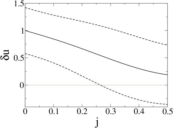
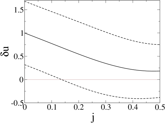
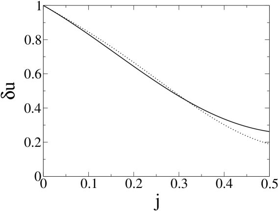
Figs. 5 and 6 show the results in the GUE ensemble for $\lambda\!=\!1$ and $3$, respectively, and Fig. 7 shows those for the GOE ensemble at $\lambda\!=\!1$. In evaluating these expressions, we use the Wigner surmise distributions for $P(x)$, which allow an analytic evaluation of $P_{0}(2j)$ and $x_{0}(2j)$. As $j$ increases, the average correction to the peak spacing decreases monotonically in all three cases. (Note, however, that our results are not completely trustworthy when $0.4\!<\!j\!<\!0.5$ because in this regime higher spin states should be taken into account.) Since $\lambda$ depends on $\xi$ and $\delta$ only logarithmically, the qualitative behavior of $\delta u(j)$ is very robust with respect to changes in charging energy, mean level spacing, or temperature.

Figure 7: Ensemble averaged correction to the “even” peak spacing as a function of strength of exchange, $j\!=\!J_{\rm s}/\Delta$, normalized by the correction at $j\!=\!0$ for $\lambda\!=\!1$. Solid: GOE. Dotted: GUE.

Figure 8: GUE ensemble averaged correction to the even peak spacing as a function of $\lambda\!=\!\ln(2E_{C}/\Delta)/\ln(\Delta/T)$ at $j\!=\!j_{0}$. The curves correspond to $j_{0}=0.3$, $0.4$, and $0.5$ from top to the bottom.

Similarly the dependence of $\delta u$ on $\lambda$ at $j\!=\!j_{0}$ is

$$\delta u(j_{0},\lambda)=\frac{\lambda\,{\mathcal{C}}(j_{0})+{\mathcal{D}}(j_{0})}{2(\lambda+1)}\;.$$ (45)

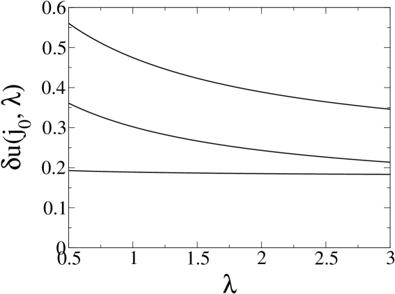
Fig. 8 shows results in the GUE case for several values of $j_{0}$. Thus for the realistic value $j_{0}\!=\!0.3$, the CEI model gives an average correction to the peak spacing which is two to three times smaller than the CI model.

7 RMS of The Correction to Peak Spacing due to Mesoscopic Fluctuations

Mesoscopic fluctuations of the correction to the peak spacing are characterized by the variance of ${\mathcal{U}}^{(2)}$. It is convenient to separate the average over the wave functions from that over the spacing $x$, writing

$$\mbox{var}\big{(}{\mathcal{U}}_{n}^{(2)}\big{)}=\sigma^{2}_{Z}\big{(}{\mathcal{U}}_{n}^{(2)}\big{)}+\sigma^{2}_{x}\big{(}{\mathcal{U}}_{n}^{(2)}\big{)},$$ (46)

where

$$\sigma^{2}_{Z}=\int_{0}^{\infty}dx\,P(x)\Big{<}\Big{(}{\mathcal{U}}_{n,S}^{(2)}-\big{<}{\mathcal{U}}_{n,S}^{(2)}\big{>}\Big{)}^{2}\Big{>}$$ (47)

is the contribution due to wave function fluctuations and

$$\sigma^{2}_{x}=\int_{0}^{\infty}\!\!dx\,P(x)\big{<}{\mathcal{U}}_{n,S}^{(2)}\big{>}^{2}-\left[\int_{0}^{\infty}\!\!dx\,P(x)\big{<}{\mathcal{U}}_{n,S}^{(2)}\big{>}\right]^{2}$$ (48)

is the contribution due to fluctuation of the spacing $x$.

We start by considering the fluctuations of the wave functions. As the number of electrons in the dot is large, the distance between the left and right dot-lead contacts is large, $\left|{\bf r}_{L}-{\bf r}_{R}\right|\gg\lambda_{F}$ where $\lambda_{F}$ is the Fermi wavelength. Therefore, the wave functions at ${\bf r}_{L}$ and ${\bf r}_{R}$ are uncorrelated [54],

$$\left<\left(Z_{kL}-1\right)\left(Z_{k^{\prime}R}-1\right)\right>=0$$ (49)

for all $k$ and $k^{\prime}$. The fluctuation of ${\mathcal{U}}^{(2)}$ can then be written entirely in terms of the properties of a single lead:

$$\Big{<}\Big{(}{\mathcal{U}}_{n,S}^{(2)}-\big{<}{\mathcal{U}}_{n,S}^{(2)}\big{>}\Big{)}^{2}\Big{>}=\frac{g_{L}^{2}+g_{R}^{2}}{\left(4\pi^{2}\xi\right)^{2}}\Big{<}\big{(}\Phi_{L,S}-\left<\Phi_{L,S}\right>\big{)}^{2}\Big{>}\;.$$ (50)

The cross terms here disappear because, according to RMT, wave functions of different energy levels are uncorrelated even at the same point in space,

$$\big{<}\left(Z_{kL}-1\right)\left(Z_{k^{\prime}L}-1\right)\big{>}=\frac{2}{\beta}\,\delta_{kk^{\prime}}$$ (51)

where $\beta\!=\!1$ ($\beta\!=\!2$) for the GOE (GUE) case. In fact, only the $k\!=\!\frac{n}{2}$ and $k\!=\!\frac{n}{2}\!+\!1$ terms contribute, as one can see by using

$$\sum_{l=1}^{\xi}\,\ln^{2}\Big{(}1-\frac{2j}{x+l}\Big{)}=O(1)$$ (52)

valid for $\xi\gg 1$. Integrating (50) over the distribution of $x$ according to Eq. (47) (keeping in mind $\xi,\delta\!\gg\!1$), we obtain

$$\sigma_{Z}^{2}\Big{(}{\mathcal{U}}_{n}^{(2)}\Big{)}=\frac{g_{L}^{2}+g_{R}^{2}}{\beta\left(4\pi^{2}\xi\right)^{2}}\big{\{}4\ln^{2}\!\xi+\left[3P_{0}(2j)+1\right]\ln^{2}\!\delta-4\left[3P_{0}(2j)-1\right]\ln\xi\ln\delta\big{\}}.$$ (53)

In the contribution to the variance due to fluctuation of the level spacing $x$, Eq. (48), $\big{<}{\mathcal{U}}_{n,S}^{(2)}\big{>}$ can be taken from the previous section. Since the average eliminates the dependence on the lead $\alpha$, we have immediately

$$\big{<}{\mathcal{U}}^{(2)}_{n,S}\big{>}^{2}=\left(\frac{g_{L}+g_{R}}{4\pi^{2}\xi}\right)^{2}\left<\Phi_{L,S}\right>^{2}$$ (54)

where $\left<\Phi_{L,S=0}\right>$ and $\left<\Phi_{L,S=1}\right>$ for $\xi,\delta\gg 1$ are given by Eq. (40). Using these expressions in Eq. (48), we obtain

$$\sigma_{x}^{2}=\left(\frac{g_{L}+g_{R}}{4\pi^{2}\xi}\right)^{2}\left({\mathcal{C}}_{\xi\xi}\ln^{2}\xi+{\mathcal{C}}_{\delta\delta}\ln^{2}\delta+{\mathcal{C}}_{\xi\delta}\ln\xi\ln\delta\right).$$ (55)

Explicit expressions for the coefficients are given below once we reach the final result.

The dependence on $g_{L}$ and $g_{R}$ of the two contributions to the variance is different. In particular, the contribution due to fluctuations of the wave functions [Eq. (53)] is proportional to

$$g_{L}^{2}+g_{R}^{2}=\frac{\left(g_{L}+g_{R}\right)^{2}}{2}+\frac{\left(g_{L}-g_{R}\right)^{2}}{2}\;.$$ (56)

The first term has the same form as the contribution (55) from fluctuations of $x$. It is convenient to write the total variance as a sum of symmetric and antisymmetric parts. Our final result for the variance is

$$\mbox{var}\big{(}{\mathcal{U}}_{n}^{(2)}\big{)}=\sigma_{s}^{2}\big{(}{\mathcal{U}}_{n}^{(2)}\big{)}+\sigma_{a}^{2}\big{(}{\mathcal{U}}_{n}^{(2)}\big{)}$$ (57)

where

$$\sigma_{s}^{2}\left({\mathcal{U}}_{n}^{(2)}\right) = \left(\frac{g_{L}+g_{R}}{4\pi^{2}\xi}\right)^{2}\Big{(}{\mathcal{S}}_{\xi\xi}\ln^{2}\xi+{\mathcal{S}}_{\delta\delta}\ln^{2}\delta+{\mathcal{S}}_{\xi\delta}\ln\xi\ln\delta\Big{)}$$ (58)

$$\sigma_{a}^{2}\left({\mathcal{U}}_{n}^{(2)}\right) = \left(\frac{g_{L}-g_{R}}{4\pi^{2}\xi}\right)^{2}\Big{(}{\mathcal{A}}_{\xi\xi}\ln^{2}\xi+{\mathcal{A}}_{\delta\delta}\ln^{2}\delta+{\mathcal{A}}_{\xi\delta}\ln\xi\ln\delta\Big{)}$$ (59)

with the coefficients $\{{\mathcal{S}}\}$ and $\{{\mathcal{A}}\}$ given by

$${\mathcal{S}}_{\xi\xi}(j) = \frac{2}{\beta}+16\left({\chi}-1\right)$$ (60)

$$+ 64\left[2jP_{0}(2j)-x_{0}(2j)\right]\left\{2j\left[1-P_{0}(2j)\right]-\left[1-x_{0}(2j)\right]\right\},$$

$${\mathcal{S}}_{\delta\delta}(j) = \frac{1}{2\beta}\left[3P_{0}(2j)+1\right]+9P_{0}(2j)\left[1-P_{0}(2j)\right],$$ (61)

$${\mathcal{S}}_{\xi\delta}(j) = -\frac{2}{\beta}\left[3P_{0}(2j)-1\right]+24\left\{x_{0}(2j)\left[1-P_{0}(2j)\right]\right.$$ (62)

$$+ \left.\left[1-x_{0}(2j)\right]P_{0}(2j)-4jP_{0}(2j)\left[1-P_{0}(2j)\right]\right\},$$

$${\mathcal{A}}_{\xi\xi}(j) = \frac{2}{\beta},~{}~{}{\mathcal{A}}_{\delta\delta}(j)=\frac{1}{2\beta}\left[3P_{0}(2j)+1\right],~{}~{}{\mathcal{A}}_{\xi\delta}(j)=-\frac{2}{\beta}\left[3P_{0}(2j)-1\right].$$ (63)

The constant $\chi$ introduced in Eq. (60) is

$${\chi}=\int_{0}^{\infty}\!\!dx\,x^{2}\,P(x).$$ (64)

For the CI model, $j=0$ and $P_{0}(0)=x_{0}(0)=1$; hence

$$\left.\mbox{var}\left({\mathcal{U}}_{n}^{(2)}\right)\right|_{j=0}=\frac{4}{\beta}\frac{g_{L}^{2}+g_{R}^{2}}{\left(4\pi^{2}\xi\right)^{2}}\left(\ln\xi-\ln\delta\right)^{2}+16\left({\chi}-1\right)\left(\frac{g_{L}+g_{R}}{4\pi^{2}\xi}\right)^{2}\ln^{2}\xi\;.$$ (65)

The first term is due to fluctuation of the wave functions at the dot-lead contacts, and the second term comes from the fluctuation of the level spacing $x$. The presence of the second term was missed in previous work [see Eq. (44b) in Ref. [43]]. If $\xi\!=\!\delta$, the first term vanishes; nonetheless, due to the second term the variance is always finite.

Figure 9: The rms of the correction to the peak spacing for the symmetric setup $g_{L}=g_{R}$ as a function of $j=J_{\rm s}/\Delta$ normalized by the ensemble averaged correction at $j=0$, Eq. (66). Solid (dotted) curve corresponds to the GOE (GUE) at $\lambda=1$. Dashed curve corresponds to the GUE at $\lambda=3$.

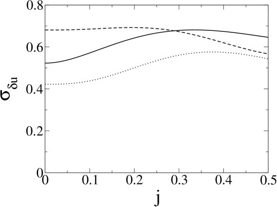
Let us consider a realistic special case of symmetric tunnel barriers, $g_{L}=g_{R}$ [44]. Then the asymmetric contribution vanishes, and the rms fluctuation of the correction to the peak spacing normalized by the average correction at $j=0$ [Eq. (42)] is

$$\sigma_{\delta u}(j)=\frac{\sigma_{s}\big{(}{\mathcal{U}}_{n}^{(2)}\big{)}}{\overline{{\mathcal{U}}_{n}^{(2)}\left(0\right)}}=\frac{\sqrt{{\mathcal{S}}_{\xi\xi}(j)\lambda^{2}+{\mathcal{S}}_{\xi\delta}(j)\lambda+{\mathcal{S}}_{\delta\delta}(j)}}{2(\lambda+1)}.$$ (66)

Fig. 9 shows this quantity plotted as a function of $j$ for both GOE and GUE. Notice that (i) the rms is of the same order as the average, and (ii) its magnitude weakly depends on $j$. To show the magnitude of the fluctuations in the correction relative to its average value, we plot two additional curves in both Fig. 5 and Fig. 6, namely $\delta u\pm\sigma_{\delta u}$. We find that at the realistic value $j\!=\!0.3$, the correction to the even peak spacing is negative for a small fraction of the quantum dots in the ensemble.

8 Conclusions

In this chapter we studied corrections to the spacings between Coulomb blockade conductance peaks due to finite dot-lead tunneling couplings. We considered both GOE and GUE random matrix ensembles of 2D quantum dots with the electron-electron interactions being described by the CEI model. We assumed $T\!\ll\!\Delta\!\ll\!E_{C}$. The $S\!=\!0$, $\frac{1}{2}$, and $1$ spin states of the QD were accounted for, thus limiting the applicability of our results to $J_{\rm s}\!<\!0.5\Delta$.

The ensemble averaged correction in even valleys is given in Eq. (41). The average correction decreases monotonically (always staying positive, however) as the exchange interaction constant $J_{\rm s}$ increases (Figs. 5-7). The behavior found is very robust with respect to the choice of RMT ensemble or change in charging energy, mean level spacing, or temperature. Our results obtained in second-order perturbation theory in the tunneling Hamiltonian are somewhat similar to the zeroth-order results [20, 7] in that the exchange interaction reduces even-odd asymmetry of the spacings between peaks. While the average correction to the even spacing is positive, that to the odd peak spacing is negative and of equal magnitude.

The fluctuations of the correction to the spacing between Coulomb blockade peaks mainly come from the mesoscopic fluctuations of the wave functions and energy level spacing $x$ in the QD. The rms fluctuation of this correction is given by Eqs. (57)-(64). It is of the same order as the average value of the correction (Figs. 5 and 6) and weakly depends on $J_{\rm s}$ (Fig. 9). Therefore, for a small subset of ensemble realizations, the correction to the peak spacing at the realistic value of $j=0.3$ is of the opposite sign. The rms fluctuation of the correction for an odd valley is the same as that for an even one.

We are aware of two experiments directly relevant to the results here. First, in the experiment by Chang and co-workers [45], the corrections to the even and odd peak spacings due to finite dot-lead tunnel couplings were measured. It was found that the even (odd) peak spacing increases (decreases) as the tunnel couplings are increased. This is in qualitative agreement with the theory, see Eq. (41). The magnitude of the effect was measured at different values of the gas parameter $r_{s}$ (and, hence $J_{\rm s}$) as well. Unfortunately, because the effect is small and the experimentalists did not focus on this issue, one can not from this work draw a quantitative conclusion about the behavior of the correction to the peak spacing as a function of $J_{\rm s}$.

Second, in the experiment by Maurer and co-workers [44], the fluctuations in the spacing between Coulomb blockade peaks were measured as a function of the dot-lead couplings with $g_{L}\!=\!g_{R}$. Therefore, only the symmetric part [Eq. (58)] would contribute to the total variance. Ref. [44] reported results for two dots: a small one with area 0.3 $\mu$m² and a large one with area 1 $\mu$m². From the area (excluding a depletion width of about 70 nm), we estimate that the large (small) dot contains about 500 (100) electrons. Measurements on the large QD found larger fluctuations upon increasing the dot-lead tunnel coupling, in qualitative agreement with the theory. Though the temperature was larger than the mean level spacing in the large QD whereas our theory is developed for $T\!\ll\!\Delta$, the theory gives about the correct magnitude for the peak spacing fluctuations. It is inconclusive whether the data is in better agreement with the CI or CEI model as the fluctuations are roughly the same (Fig. 9) in both. In the small QD, there is an anomaly for the strongest coupling in the experiment – the fluctuations suddenly decrease. In addition, the experimental fluctuations are one order of magnitude larger than the theoretical estimate [Eqs. (66) and (42)]. The reason for this discrepancy is not clear at this time. Possible contributing factors include scrambling of the electron spectrum as the charge state of the dot changes, or the role of the fluctuations when the dot is isolated (i.e., fluctuations in ${\mathcal{U}}^{(0)}$). In order to assess quantitatively the role of dot-lead coupling in the Coulomb blockade, further experiments are needed.

Chapter 3 Introduction to Quantum Computation with Quantum Dots

1 Overview

This chapter serves as an introduction to the field of quantum computation (QC). The plan of the chapter is as follows. In Section 2 we explain why QC field deserves our attention. In Section 3 we outline the mathematical basis of quantum computations. In Section 4 we list and briefly explain DiVincenzo’s criteria of physical implementation. Finally, in Section 5 we briefly mention liquid state NMR quantum computing proposal but mostly concentrate on the spintronic quantum dot proposal put forth by Loss and DiVincenzo [55].

2 Introduction to Quantum Computation

Quantum computation (QC) holds out tremendous promise for efficiently solving some of the most difficult problems in computational science: integer factorization [56], discrete logarithms, and modeling of quantum mechanical systems [57]. These problems are intractable on any present or future conventional computer.

The fact that quantum systems can perform a computation was realized in 1982 by Paul Benioff and Richard Feynman. In 1994 Peter Shor proved that quantum computer can perform prime factoring in polynomial time as compared to the classical one which requires exponential time to solve this problem [56]. The prime factoring problem is defined as follows: given number $N$ which we know is a product of two primes $P$ and $Q$, find $P$ and $Q$. Table 1 gives one a flavor on how computation times scale with the complexity of the factoring problem for classical and quantum computers. As one can see for the 400-digits prime factoring problem even relatively small quantum computer will do much better than a network of hundreds classical computers. This is attained due to quantum parallelism discussed in the next section.

	Quantum Computer	Classical Computer:
	of 70 Qubits	Network of
	(Shor’s Algorithm)	Hundreds Workstations
130-Digits Number	1 Month	1 Month
Factoring
400-Digits Number	3 Years	$10^{10}$ Years
Factoring		(Age of The Universe)

Table 1: Quantum computer vs. network of hundreds classical computers: Scaling of the computational time with the complexity of the factoring problem.

Shor’s spectacular result attracted to the field of QC many physicists and computer scientists alike. Many proposals for physical realization of QC have been put forth since then. New experimental techniques were developed to control phase coherence of the quantum mechanical systems on a nano scale.

Since prime factoring is the most secure encryption scheme in wide use today, the field of QC enjoyed significant funding from government agencies in the USA, EU, and Australia.

3 Mathematical Basis of Quantum Computations

In this section we review the mathematical basis of quantum computations.

1 Quantum Bits and Entangled States

The bits of information in a quantum computer are formed by two orthogonal states of a two-level quantum mechanical system $\left|0\right>$ and $\left|1\right>$, Fig. 1. To distinguish between classical and quantum bits quantum bit was given a special name: qubit.

Figure 1: Schematic picture of the quantum bit.

For example, a nucleus of spin-$\frac{1}{2}$ (or an electron) can serve as a natural qubit: $\left|0\right>=\left|\downarrow\right>$, $\left|1\right>=\left|\uparrow\right>$. In contrast to the classical bit, qubit has the following properties [58]:
(i) The states $\left|0\right>$ and $\left|1\right>$ do not constitute all possible states of a qubit. In fact, it can be in an arbitrary superposition state: $\left|\chi\right>=\alpha\left|0\right>+\beta\left|1\right>$, where $\alpha$ and $\beta$ are complex numbers with $\left|\alpha\right|^{2}+\left|\beta\right|^{2}=1$ constraint.
(ii) Entangled state of two qubits is possible, e.g.:

$$\left|\psi\right>=\frac{1}{\sqrt{2}}\left(\left|0\right>_{1}\otimes\left|0\right>_{2}+\left|1\right>_{1}\otimes\left|1\right>_{2}\right).$$ (1)

In this state each individual qubit fails to have any state of its own. The information is, therefore, encoded only in the correlation between the qubits 1 and 2. Two qubits in an entangled state are also called EPR pair [59].

2 Steps in Quantum Computation and Quantum Gates

To perform quantum computation we should [58]
(i) Prepare a collection of $n$ qubits in the appropriate initial state at $t=0$: $\left|\psi(0)\right>$. The initial state is usually taken to be

$$\left|\psi(0)\right>=\left|0\right>_{1}\otimes\left|0\right>_{2}\otimes\,\dots\,\otimes\left|0\right>_{n}$$ (2)

or a state constructed from this one by application of the appropriate unitary transformations.
(ii) Let that state evolve under the appropriate unitary transformation $U$. $U$ can be realized as the ordinary time evolution of a physical system with appropriately constructed time-dependent Hamiltonian $H(t)$:

$$\left|\psi(t)\right>=U\left|\psi(0)\right>=Te^{-i\int_{0}^{t}d\tau H(\tau)}\left|\psi(0)\right>.$$ (3)

(iii) Extract the result of the computation by appropriate measurement on the final state. Typical final measurement is made on a subset of individual qubits.

Among all possible unitary transformations there are those acting on a single qubit, a pair of qubits, a set of three qubits, etc. Let us call unitary transformations acting only on a single qubit or a pair of qubits quantum gates. In 1995 Barenco and coworkers proved that any quantum computation algorithm can be decomposed in a series of quantum gates: single qubit and two-qubit XOR gates [60].

3 Quantum Parallelism

The computational basis of $n$-qubit quantum computer is formed by $2^{n}$ states like this one:

$$\left|0\right>_{1}\otimes\left|0\right>_{2}\otimes\left|0\right>_{3}\otimes\left|0\right>_{4}\otimes\,\dots\,\otimes\left|0\right>_{n-3}\otimes\left|1\right>_{n-2}\otimes\left|1\right>_{n-1}\otimes\left|1\right>_{n}.$$ (4)

Each qubit in this ket-vector can be in one of the two possible eigenstates. Let us denote ket-vector like the one in Eq. (4) simply as $\left|x\right>$, where $x$ is the integer between $0$ and $2^{n}-1$, whose binary expansion gives the corresponding ket-vector. For example, in the case of Eq. (4) the binary expansion is $0000\dots 0111$. It corresponds to $\left|x\right>=\left|7\right>$.

The concept of quantum parallelism can be illustrated as follows [58]. Consider certain two-qubit entangled state and act on it with a quantum gate $\,{\mathcal{U}}$. Since unitary transformations are linear we obtain:

$${\mathcal{U}}\left(\frac{1}{\sqrt{3}}\left|0\right>_{1}\otimes\left|0\right>_{2}+\sqrt{\frac{2}{3}}\left|1\right>_{1}\otimes\left|1\right>_{2}\right)=\frac{1}{\sqrt{3}}~{}{\mathcal{U}}\left|0\right>_{1}\otimes\left|0\right>_{2}+\sqrt{\frac{2}{3}}~{}{\mathcal{U}}\left|1\right>_{1}\otimes\left|1\right>_{2}.$$ (5)

Two important remarks should be made about Eq. (5): (i) as a result of quantum computation we obtained the same superposition in the final state as we had in the initial state and (ii) we performed quantum computation on all input states simultaneously! This property of quantum computation is called quantum parallelism. Quantum parallelism gives quantum computer the potential to do tricks that a classical computer can perform only with significantly greater computational effort.

Suppose we have a unitary transformation ${\mathcal{U}}_{f}$, associated with a function $f$. Function $f$ replaces a computational basis state $\left|x\right>$ by $\left|f(x)\right>$, where $f(x)$ can take the following integer values: $f(x)=0,1,2,\dots,2^{n}-1$. Since ${\mathcal{U}}_{f}$ is a unitary transformation, it is invertible. Hence, function $f$ is bijective – its action is nothing but a permutation of integers $\{x\}$. This restriction on the nature of $f$ is excessively strong. Therefore, let us double the number of qubits and define ${\mathcal{U}}_{f}$ on the $2n$-qubit space as follows:

$$\left|x\right>\otimes\left|0\right>\,\stackrel{{\scriptstyle{\mathcal{U}}_{f}}}{{\longrightarrow}}\,\left|x\right>\otimes\left|f(x)\right>.$$ (6)

Let us call the first set of $n$-qubits input register and the second set of $n$-qubits output register [58].

To illustrate the concept of quantum parallelism even further let us take the input register to be in the state

$$\left|s\right>=\frac{1}{2^{n/2}}\sum_{x=0}^{2^{n}-1}\left|x\right>=\frac{1}{\sqrt{2}}\left(\left|0\right>_{1}+\left|1\right>_{1}\right)\otimes\,\dots\,\otimes\frac{1}{\sqrt{2}}\left(\left|0\right>_{n}+\left|1\right>_{n}\right).$$ (7)

This input state can be obtained from the state in Eq. (2) by subjecting each qubit to the one-qubit gate that “rotates” each “spin” 90 degrees about the $y$-axis. Under the action of ${\mathcal{U}}_{f}$

$$\left|s\right>\otimes\left|0\right>=\frac{1}{2^{n/2}}\sum_{x=0}^{2^{n}-1}\left|x\right>\otimes\left|0\right>\,\stackrel{{\scriptstyle{\mathcal{U}}_{f}}}{{\longrightarrow}}\,\frac{1}{2^{n/2}}\sum_{x=0}^{2^{n}-1}\left|x\right>\otimes\left|f(x)\right>.$$ (8)

Notice what just happened: in one run we calculated $f(x)$ on all $2^{n}$ possible inputs. If we would have 100 qubits in our input register, then $f(x)$ would have been simultaneously calculated on $2^{100}\approx 10^{30}$ different inputs. This massive quantum parallelism is well outside the reach of any classical computer.

4 Important Remarks

Useful information has to be extracted from the output of the quantum computation, see Eq. (8). To illustrate how the measurement process works let us perform a measurement on the final state in Eq. (8). Namely, let us measure the individual states of all qubits in the input and output registers. With the equal probability of $2^{-n}$ one can find any state of the input register. Let us assume that we find $\left|x_{0}\right>$ as a result of the measurement on the input register. Then the result of the measurement on the output register is $\left|f(x_{0})\right>$. Thus, we calculated the value of $f(x_{0})$ at the randomly chosen $x_{0}$. All other information has been lost because we collapsed the whole superposition in Eq. (8) onto a single component $\left|x_{0}\right>\otimes\left|f(x_{0})\right>$.

If Eq. (8) was the only quantum algorithm one could come up with, one would be no better off than just doing single classical computation on a randomly chosen input. Therefore, the goal of designing quantum algorithms is to have easily accessible data of interest in the final state and to make sure that the data can not be generated by a classical algorithm without enormously greater computational effort. The first algorithm which satisfies these conditions was created by Peter Shor for the prime factoring problem.

The other difficulty is to maintain the coherence of an entangled state of many qubits. Unfortunately, it is impossible to completely isolate our qubits from the environment during a quantum computation. The coupling to the environment leads to decoherence or collapse of the quantum state which is especially severe for the entangled states of many qubits. The solution to this challenge is to use quantum error-correcting codes [61]. We know that these codes can work only for the sufficiently small decoherence rates. Therefore, one of the main problems in physical realization of the quantum computer is how to reduce decoherence due to different couplings to the environment.

4 DiVincenzo’s Criteria of Physical Implementation

Five DiVincenzo’s criteria [62] serve as a general guidance to the physical implementation of a working scalable quantum computer. They naturally follow from the mathematical basis of QC discussed in the previous section and can be formulated as follows:
(i) A collection of the quantum mechanical two-level systems (qubits) is needed. Each qubit should be separately identifiable and externally addressable. One should be able to add qubits at will.
(ii) It should be possible to completely (or with very high accuracy) decouple qubits from one another. One should be able to set the state of each qubit to $\left|0\right>$ in the beginning of each computation.
(iii)  Long decoherence times are required. For the error correcting-codes to be applicable decoherence time should be at least 4 orders of magnitude larger than the “clock time” of the quantum gates.
(iv) Logic operations should be doable. For example, two-body Hamiltonians involving nearby qubits should be under independent and precise external control. One should be able to smoothly (on the time scale of one clock cycle) turn these Hamiltonians on and off. The integral of the pulse should be controlled with the accuracy of at least 1 part in $10^{4}$.
(v) Projective quantum measurements on the qubits must be doable. It is useful, though not necessary, for these measurements to be doable fast (that is, within few clock cycles) and have high quantum efficiency (otherwise quantum computation has to be done in an ensemble style).

5 Quantum Computing Proposals

1 Liquid State NMR

Since the original work by Peter Shor many quantum computing proposals were put forth in different areas of physics. At the time of writing liquid state nuclear magnetic resonance (NMR) proposal is well ahead of its competition. In the experiment by Vandersypen and coworkers [63] the custom-synthesized molecule (used as the quantum computer) contained five ${}^{19}F$ and two ${}^{13}C$ spin-$\frac{1}{2}$ nuclei as qubits. The quantum gates were realized by a sequence of spin-selective radio-frequency pulses. The readout was performed via NMR spectroscopy. For the first time the simplest instance of Shor’s algorithm: factorization of 15 ($15=3\times 5$) was demonstrated [63].

Unfortunately, liquid state NMR proposal lacks scalability, see the first DiVincenzo’s criterion. Indeed, to realize more complicated algorithms one has to design and synthesize new molecules.

2 Spintronic Quantum Dot Proposal by Loss and DiVincenzo

The experimental progress in solid state QC proposals falls significantly behind liquid state NMR proposal. Nonetheless, once the universal gates (one- and two-qubit quantum gates) become sufficiently error free the scaling of the quantum computer is going to be more or less straightforward. Among different solid state QC proposals one can distinguish three major categories: (i) superconducting microcircuits containing Josephson junctions [64, 65], (ii) nuclear spins of the impurity atoms in semiconductor QDs [66], and (iii) electron spin- or charge-qubits in semiconductor QDs, see Chapters 4 and 6 for the references. Charge qubit in the semiconductor double QD are discussed in Chapter 6.

Figure 2: Schematic picture of the spintronic QD proposal by Loss and DiVincenzo. 2D electron gas is confined on the interface of AlGaAs/GaAs heterostructure. The electrodes deposited on top of the heterostructure control the shape of the QDs and their tunnel couplings to each other. Back gates control the electron numbers in each dot. Magnetized layer is needed to realize one-qubit operations. Copyright by G. Burkard, H.-A. Engel, and D. Loss, from Ref. [67].

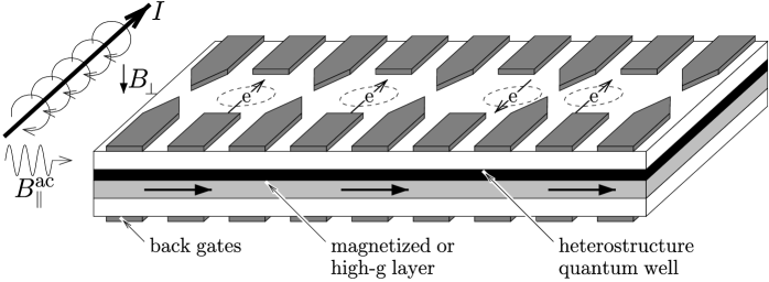
Here we describe the original spintronic quantum dot proposal by Loss and DiVincenzo [55, 62]. They consider an array of coupled 2D lateral quantum dots, see Fig. 2. Each QD should contain odd number of electrons so that spin of an electron on the last occupied orbital serves as a natural qubit: $\left|0\right>=\left|\downarrow\right>$ and $\left|1\right>=\left|\uparrow\right>$.

Let us briefly go over five DiVincenzo’s criteria to see if this system satisfies them and what is needed to be improved as compared to the modern experimental technologies.

Criterion (i). We have a collection of two-level quantum mechanical systems and we can add to the system as many new qubits as we want.

For the qubit to be separately identifiable the corresponding quantum dot should contain odd number of electrons with sufficiently high accuracy. This electron number can be adjusted by back-gate electrode voltages shown in Fig. 2. To make sure that the number of electrons is odd and hence spin of the QD is equal to $\frac{1}{2}$ one can employ zero-bias anomaly measurement in transport through the QD which signals a Kondo effect.

Criterion (ii). To set the state of each qubit to $\left|0\right>$ it is sufficient to place the spins in the magnetic field of several Tesla at the liquid-He temperature. For this $\left|0\right>\otimes\left|0\right>\otimes\dots\otimes\left|0\right>$ state to be stable upon removal of the magnetic field the qubits must be decoupled from one another to a very high accuracy. This can be achieved by setting the pairs of electrodes between neighboring QDs to high negative voltages so that the orbital wave-functions overlap is negligible.

Criterion (iii). The experiments on the precession of the electron spin in a variety of semiconductor materials were performed by Kikkawa and Awschalom [68]. In some structures they found spin decoherence times $\tau_{\phi}$ up to hundreds of nanoseconds, that is, at least one order of magnitude larger than charge decoherence times. These results are quite encouraging. However spin decoherence times are expected to be very device- and structure-specific. Therefore, more experiments especially on the QD array setups are necessary.

One must emphasize that what really matters is the ratio $\tau_{\phi}/\tau_{s}$, where $\tau_{s}$ denotes the clock cycle time which will be defined below.

Criterion (iv). To physically realize one-qubit quantum gates it must be possible to subject a specified qubit to the localized magnetic field of proper direction and strength. This can be done by using a scanned magnetic particle or by the use of magnetized barrier material that the electron can be inserted in and out of by electric gating, see Fig. 2. The experimental realization of both of these ideas is going to be quite challenging, especially, taking into account the fact that the required accuracy is 1 part in $10^{4}$.

Fortunately, according to the paper by DiVincenzo and coworkers [69] one can completely eliminate one-qubit quantum gates at the expense of increasing the size of the logical qubit from one to three QDs. In this scheme two-body Hamiltonians is the only building block necessary to realize quantum computations.

These two-body Hamiltonians, or two-qubit quantum gates if we go back to the original Loss and DiVincenzo proposal, can be realized by increasing the voltages on the electrodes between neighboring QDs. When these voltages are increased the potential barrier between neighboring QDs is lowered and the electron wave-functions overlap, see two right-most QDs in Fig. 2. This leads (with high accuracy) to the effective spin-spin Heisenberg interaction $J\,{\bf S}_{i}\,{\bf S}_{i+1}$ with $J\approx 4\,t^{2}/U$, where $t$ is the tunneling matrix element determined by the overlap of the electron wave-functions in neighboring QDs and $U$ is the Coulomb on-site repulsion energy. The corresponding “clock time” can be estimated as follows: $\tau_{s}\sim 1/J$ ($\hbar=1$).

For the error-correcting codes to be applicable Heisenberg spin-spin interaction $J\,{\bf S}_{i}\,{\bf S}_{i+1}$ has to be valid with the accuracy of $10^{-4}$. Besides, to avoid correlated errors $J$ should be sufficiently small in the “off” state of the two-body Hamiltonian. One major source of errors is the mesoscopic fluctuations. They appear in both the tunneling matrix element $t$ and the relative position of the energies of the last occupied orbitals in neighboring QDs. In Chapter 4 we find that the constraint of having small errors implies keeping accurate control, at the few percent level, of several electrode voltages.

The other technical problem is to control the area under the two-qubit gate pulse with the accuracy of $10^{-4}$. Especially, taking into account the fact that the pulse should be adiabatic on the time scale of tens of picoseconds so that electrons are not excited to the higher-lying energy levels. This issue is also discussed in details in Chapter 4.

Criterion (v): A significant progress has been made recently in the one electron spin readout technique [70, 71]. Kouwenhoven and coworkers have demonstrated single-shot read-out of single- and two-electron spin states in a QD. An electron was allowed to escape from the QD or not depending on its spin state (the tunneling was energetically allowed only for the higher energy state). The charge of the QD was then measured using a quantum point contact located near the QD. With this technique they obtained 65% measurement visibility (the corresponding fidelity was 82.5%). In the other slightly modified scheme they obtained even better values for the visibility and fidelity: 80% and 90%, respectively. Thus, high quantum efficiency of the measurement is reached.

The readout time in the experiment was about $0.5\,$ms, whereas the energy relaxation time $T_{1}\sim 0.85\,$ms. Although not in principle necessary, it would be useful for the implementation of the error-correcting codes to reduce the readout time to about one hundreds of $T_{1}$ time.

In conclusion, more experiments are on the way. In particular, Kouwenhoven and coworkers are planning to realize swapping of the spin states in adjacent quantum dots. Since two-body Hamiltonian is the main building block of the spin based quantum computer these experiments will provide a valuable inside into possible directions of the future research.

Chapter 4 Spin Qubits in Multi-Electron Quantum Dots

1 Overview

In this chapter we study the effect of mesoscopic fluctuations on the magnitude of errors that can occur in exchange operations on quantum dot spin-qubits. Mid-size double quantum dots, with an odd number of electrons in the range of a few tens in each dot, are investigated through the constant interaction model using realistic parameters. It is found that the constraint of having short pulses and small errors implies keeping accurate control, at the few percent level, of several electrode voltages. In practice, the number of independent parameters per dot that one should tune depends on the configuration and ranges from one to four.

The work in this chapter was done in collaboration with Eduardo R. Mucciolo and Harold U. Baranger.

2 Introduction

Since the discovery that quantum algorithms can solve certain computational problems much more efficiently than classical ones [56, 72], attention has been devoted to the physical implementation of quantum computation (QC). Among the many proposals, there are those based on the spin of electrons in laterally confined quantum dots (QD) [55], which may have great potential for scalability and integration with current technologies. For any successful proposal, one must be able to perform single- and double-qubit operations much faster than the decoherence time. In fact, all logical operations required for QC can be realized if these elementary operations are sufficiently error free [60].

Single qubit operations involving a single QD will likely require precise engineering of the underlying material or control over local magnetic fields [62]; both have yet to be achieved in practice. Two-qubit operations, in contrast, are already within experimental reach. They can be performed by sending electrical pulses to modulate the potential barrier between adjacent QDs. That permits direct control over the effective, Heisenberg-like, exchange interaction between the qubit spins, which is created by the overlap between the electronic wave-functions of the QDs [55]. These operations are important elements in forming a basic two-qubit gate such as the controlled-not [73] and in the propagation of quantum information through QD arrays [55]. In fact, using three QDs instead of just one to form a logical qubit would allow one to perform all logical operations entirely based on the exchange interaction [69]. Thus, exchange operations will likely play a major role in the realization of QD qubits. A quantitative understanding of errors that occur during an exchange operation will help in designing optimal systems.

The first proposal for a QD spin qubit [55] relied on having a single electron in a very small laterally confined QD. One advantage of such a system is that the Hilbert space is nominally two-dimensional. Leakage from the computational space involves energies of order either the charging energy or the single-particle excitation energy, both of which are quite large in practice ($\sim 1$ meV $\sim 10$ K). Working adiabatically – such that the inverse of the switching time is much less than the excitation energy – assures minimal leakage. The large excitation energy implies that pulses of tens of picoseconds would be both well within the adiabatic regime and below the dephasing time $\tau_{\phi}$ (which is typically in the nanosecond range since orbital degrees of freedom are involved). However, in practice, it is difficult to fabricate very small tunable devices [74]. Moreover, one-electron QDs may offer little possibility of gate tuning due to their rather featureless wave functions.

Alternatively, a qubit could be formed by the top most “valence” electron in a QD with an odd number of electrons [75]. In this case, electrons filling the lower energy states should comprise an inert shell, leaving as the only relevant degree of freedom the spin orientation of the valence electron. Large QDs with 100-1000 electrons, while much simpler to fabricate than single electron QDs, are unsuitable because the excitation energy is small ($\sim 50\,\mu$eV $\sim 0.6$ K), leading to leakage or excessively slow exchange operations. On the other hand, mid-size QDs, with 10-40 electrons, are sufficiently small to have substantial excitation energies, yet both reasonable to fabricate and tunable through plunger electrodes. For these dots, a careful analysis of errors is necessary.

Perhaps the best example of an exchange operation is the swap of the spin states of the two qubits. For instance, it causes up-down spins to evolve to down-up. Maximum entanglement between qubits occurs when half of a swap pulse takes place – a square-root-of-swap operation. Several authors have treated the problem of swap errors in QD systems [76, 77, 78, 79, 80, 81]. A primary concern was the occurrence of double occupancy (when both valence electrons move into the same QD) during and after the swap. However, no study so far has considered another intrinsic characteristic of electronic states in multi-electron QDs, namely, their marked dependence on external perturbations such as electrode voltage or magnetic field. This sensitivity gives rise to strong sample-to-sample fluctuations arising from the phase-coherent orbital motion [5]. These features can make the precise control of energy levels, wave functions, and inter-dot couplings a difficult task.

In this chapter we study errors and error rates that can take place during the exchange operation of two spin qubits based in multi-electron QDs. We consider realistic situations by taking into account an extra orbital level and fluctuations in level positions and coupling matrix elements. These lead to deviations from a pre-established optimal swap operation point, especially when a single-particle level falls too close to the valence electron level. Reasons for such fluctuations can be, for instance, (i) the lack of a sufficient number of tuning parameters (i.e., plunger electrodes), or (ii) the cross-talk between the tuning electrodes. Our results set bounds on the amount of acceptable detuning for mid-size QD qubits.

This chapter is organized as follows. In Section 3, we introduce and justify the model Hamiltonian. The states involved in the exchange operation are presented in Section 4, where we also discuss the pulses and the parameters involved in the exchange operations. In Section 5 we present the results of our numerical simulations. We also discuss the impact of mesoscopic effects on errors and put our analysis in the context of actual experiments. Finally, in Section 6 we draw our conclusions.

3 Model System

We begin by assuming that the double QD system can be described by the Hamiltonian [12]

$$H=H_{A}+H_{B}+H_{AB},$$ (1)

where

$$H_{\alpha}=\sum_{j,\sigma}\epsilon_{j}^{\alpha}\,n_{\alpha,j\sigma}+\frac{U_{\alpha}}{2}\sum_{j,\sigma}n_{\alpha,j\sigma}\Big{(}\sum_{k,\sigma^{\prime}}n_{\alpha,k\sigma^{\prime}}-1\Big{)},$$ (2)

$\alpha=A,B$, and

$$H_{AB}=\sum_{j,k,\sigma}\left(t_{jk}\,a_{j\sigma}^{\dagger}b_{k\sigma}+\text{h.c.}\right).$$ (3)

Here, $n_{A,j\sigma}=a^{\dagger}_{j\sigma}a_{j\sigma}$ and $n_{B,k\sigma}=b^{\dagger}_{k\sigma}b_{k\sigma}$ are the number operators for the single-particle states in the QDs (named $A$ and $B$), $\epsilon^{\alpha}_{j}$ denotes the single-particle energy levels, $t_{jk}$ are the tunneling amplitudes between the dots, and $U_{\alpha}$ is the charging energy ($\sigma=\uparrow,\downarrow$ and $j,\,k$ run over the single-particle states). Typically, for mid- to large-size QDs, the charging energy is larger than the mean level spacing.

In the literature of Coulomb blockade phenomena in closed QDs, the Hamiltonian in Eq. (2) is known as the constant interaction model. It provides an excellent description of many-electron QDs, being supported by both microscopic calculations and experimental data [5, 12, 82, 20, 7, 83, 84]. The reasoning behind its success can be understood from two observations. First, mid- to large-size QDs, with more than ten electrons, behave very much like conventional disordered metals in the diffusive regime. Wavelengths are sufficiently small to resolve irregularities in the confining and background potentials, leading to classical chaos and the absence of shell effects in the energy spectrum. In this case, the single-particle states obey the statistics of random matrices, showing complex interference patterns and resembling a random superposition of plane waves. This is in contrast with the case of small, circularly symmetric, few-electron QDs, where shell effects are pronounced [75, 85].

Second, for realistic electron densities, the QD linear size is larger than the screening length of the Coulomb interactions. In the presence of random plane waves, the screened interaction can then be broken up into a leading electrostatic contribution characterized by the QD capacitance plus weak inter-particle residual interactions [12, 84]. This description becomes more accurate as the number of electrons gets larger since the residual interactions become weaker. The electron bunching is reduced as wave functions become more uniformly extended over the QD. Also, the increase in the number of oscillations in the wave functions leads to a self-averaging of the residual interactions. In this limit, one arrives at the so-called “universal Hamiltonian” for QDs, containing only single-particle levels, the charging energy, and a mean-field exchange term [5, 12]. This Hamiltonian can be derived explicitly via a random-phase approximation treatment of the Coulomb interaction and the use of random-matrix wave functions [12, 84].

According to these arguments, interaction effects beyond the charging energy term are omitted in Eq. (2). In addition, the intra-dot exchange interaction, which tends to spin polarize the QD, is also neglected. The reason for that is the following. One can show that the intra-dot exchange term only affect states where there is double occupancy of a level. Thus, the exchange interaction constant always appears side-by-side with the charging energy. But in multi-electron dots, the exchange energy (which is at most of order of the mean level separation) is much smaller than the charging energy. Thus, intra-dot exchange effects are strongly suppressed by the charging energy. We have verified that their inclusion does not modify appreciably our final results. We expect the exchange interaction to become important for two-qubit operations only in the case of small QDs with only a few electrons, when all energy scales (including the mean level spacing) are of the same order.

Thus, the simple picture where single-particle states are filled according to the Pauli principle up to the top most level is an appropriate description of multi-electron dots [5, 12, 82, 20, 7, 83, 84]. In order to define the spin-$\frac{1}{2}$ qubits, both QDs should contain an odd number of electrons (say, $2N_{A}-$1 and $2N_{B}-$1). The QD spin properties are then dictated by the lone, valence electron occupying the highest level. The remaining electrons form an inert core, provided that operations are kept sufficiently slow so as not to cause particle-hole excitations to other levels.

Experimentally, the two-qubit exchange operations also require the capability of isolating the QDs from each other, so that a direct product state can be prepared, such as

$$|i\rangle=|N_{A},\uparrow\rangle_{A}\otimes|N_{B},\downarrow\rangle_{B},$$ (4)

where the kets represent only the spin of the valence electron on each QD.

4 Errors in Exchange Operations

We focus our study on errors that appear after a full swap operation (which should result in no entanglement). Although it could in principle seem more sensible to look at the square-root-of-swap operation (which creates entanglement and is therefore a building block of logical gates), error magnitudes for the latter are straightforwardly related to those of the full swap operation, as we will show. We leave the discussion of the square root of swap to Section 5.

The ideal full swap operation exchanges the valence electrons of the QD system. For instance, it takes the product state $|i\rangle$ into

$$|f\rangle=\hat{U}_{\text{sw}}\,|i\rangle=|N_{A},\downarrow\rangle_{A}\otimes|N_{B},\uparrow\rangle_{B}.$$ (5)

Physically, the full swap can be implemented by starting with isolated QDs, turning on the inter-dot coupling for a time $T$ (the pulse duration), and then turning it off, isolating the QDs again. For weakly coupled QDs ($|t|\ll U,\delta\epsilon$), one finds $T\approx(\pi/4)\,U/|t|^{2}$, where $t$ and $U$ here represent typical values for the coupling matrix element and the charging energy, respectively (throughout we assume $\hbar=1$). To quantify the amount of error that takes place during the operation, we use the probability of not reaching $|f\rangle$ asymptotically, namely,

$$\varepsilon=1-|\langle f|\psi(+\infty)\rangle|^{2}.$$ (6)

Figure 1: Schematic disposition of energy levels of a system of two QD spin qubits (only levels close to the top occupied state are shown). The dashed lines indicate the most probable transitions that can occur during the exchange operation.

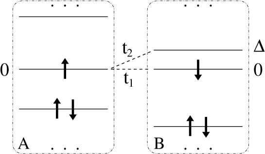
We solved numerically the time-dependent Schrödinger equation that derives from Eq. (1) for the particular but nevertheless realistic case shown in Fig. 1. We assumed that voltage tuning allows one to place the top most electron of QD $A$ into an isolated single-particle state of energy $\epsilon^{A}_{N_{A}}=0$ aligned with the energy of the top most electron in QD $B$, $\epsilon^{B}_{N_{B}}=0$. However, limited tuning ability leaves an adjacent empty state close in energy in QD $B$: $\epsilon^{B}_{N_{B}+1}=\Delta$. Therefore, while we can approximately neglect all levels but one in QD $A$, for QD $B$ we needed to take two levels into account, having hopping matrix elements denoted by $t_{1}=t_{N_{A}N_{B}}$ and $t_{2}=t_{N_{A},N_{B}+1}$. To facilitate the analysis, we assumed that the dots have the same capacitance, $C$, so that $U_{A}=U_{B}=U=e^{2}/C$.

The Hamiltonian of Eq. (1) conserves total spin. Assuming that filled inner levels in both QDs are inert (forming the “vacuum” state $|0\rangle$), we can span the $S_{z}=0$ Hilbert subspace with nine two-electron basis states. According to their transformation properties, they can be divided into “singlet”

$$|S_{l}\rangle = \frac{1}{\sqrt{2}}\left(b_{N_{B}+l-1,\downarrow}^{\dagger}a_{N_{A}\uparrow}^{\dagger}-b_{N_{B}+l-1,\uparrow}^{\dagger}a_{N_{A}\downarrow}^{\dagger}\right)|0\rangle,$$

$$|D_{l}\rangle = b_{N_{B}+l-1,\downarrow}^{\dagger}b_{N_{B}+l-1,\uparrow}^{\dagger}|0\rangle,$$ (7)

$$|D_{3}\rangle = \frac{1}{\sqrt{2}}\left(b_{N_{B}+1,\downarrow}^{\dagger}b_{N_{B}\uparrow}^{\dagger}-b_{N_{B}+1,\uparrow}^{\dagger}b_{N_{B}\downarrow}^{\dagger}\right)|0\rangle,$$

$$|D_{4}\rangle = a_{N_{A}\downarrow}^{\dagger}a_{N_{A}\uparrow}^{\dagger}|0\rangle,$$

and “triplet”

$$|T_{l}\rangle = \frac{1}{\sqrt{2}}\left(b_{N_{B}+l-1,\downarrow}^{\dagger}a_{N_{A}\uparrow}^{\dagger}+b_{N_{B}+l-1,\uparrow}^{\dagger}a_{N_{A}\downarrow}^{\dagger}\right)|0\rangle,$$

$$|D_{5}\rangle = \frac{1}{\sqrt{2}}\left(b_{N_{B}+1,\downarrow}^{\dagger}b_{N_{B}\uparrow}^{\dagger}+b_{N_{B}+1,\uparrow}^{\dagger}b_{N_{B}\downarrow}^{\dagger}\right)|0\rangle,$$ (8)

classes, with $l=1,2$.

The final states that correspond to an error have either double occupancy ($|D_{k}\rangle$, $k=1,\ldots,5$), or an electron in the $(N_{B}+1)$-level of QD $B$ ($|S_{2}\rangle$ and $|T_{2}\rangle$). In addition, a return to the initial state is also considered an error. It is worth noticing the difference between our treatment of the problem and that of Ref. [80]. In our case, errors come mainly from either ending in the excited single-particle state after the operation is over (i.e., states $|S_{2}\rangle$ and $|T_{2}\rangle$), or from “no-go” defective operations. In Ref. [80], errors come from having double occupancy in the final state. Double occupancy errors can be exponentially suppressed by adiabatically switching the pulse on and off on time scales larger than the inverse charging energy [55, 77, 78, 80]. Making pulses adiabatic on the time scale of the inverse mean level spacing for multi-electron quantum dots is more challenging, especially because the spacings fluctuate strongly both from quantum dot to quantum dot and upon variation of any external parameter (mesoscopic fluctuations). Therefore, multi-electron quantum dots require extra tunability to get around such problems.

Very small errors, below $10^{-6}$–$10^{-4}$, can, in principal, be fixed by the use of error correction algorithms [61]. The pulses, therefore, should be sufficiently adiabatic for errors to remain below this threshold. We adopted the following pulse shape:

$$v(t)=\frac{1}{2}\left(\tanh\frac{t+T/2}{2\tau}-\tanh\frac{t-T/2}{2\tau}\right),$$ (9)

where $\tau$ is the switching time. The pulse will remain both well-defined and adiabatic provided that $T\gg\tau\gg\text{max}\{\Delta^{-1},U^{-1}\}$. Notice that this pulse is equivalent to that adopted in Ref. [80] up to exponential accuracy, $O(e^{-T/\tau})$, with $T\gg\tau$. There is no particular reason to believe that either performs better than the other; our choice was dictated by technical convenience.

Figure 2: Full swap error as a function of upper level detuning in quantum dot $B$. The pulse width is optimized for $\Delta=1$, $\tau=6$, and $t_{1,2}=0.2$. Results for different charging energies are shown. Interference between different quantum mechanical paths in the device causes a sharp minimum.

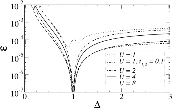
5 Results

We used a standard numerical method, the so-called Richardson extrapolation [86], to solve the Schrödinger equation for $|\psi(t)\rangle$. The first step in our analysis was to find the optimal value of $T$ which minimized the full swap error, as defined in Eq. (6), for a given set of parameters $U$, $t_{1}$, and $\tau$ (we used $\Delta=1$ and took $t_{2}=t_{1}$). The second step was to study how this minimal error depends on $\tau$. There is actually an optimal interval for $\tau$, since small switching times spoil adiabaticity, while large ones compromise the pulse shape (when $T$ is relatively short). Empirically, we find that errors related to switching times become negligible once $\tau$ reaches values of about $\tau_{0}=4\,\text{max}\{\Delta^{-1},U^{-1}\}$, provided that $\tau\ll T$. In what follows, we fix $\tau\geq\tau_{0}$.

1 Mesoscopic Effects

Figure 2 shows the full swap error as a function of $\Delta$ when $T$ is fixed to its optimal value for $\Delta=1$. Such a situation would arise experimentally if the pulse is optimized for a certain configuration, but a fluctuation in level spacing occurs. Notice the sharp increase in error as $\Delta$ decreases. While increasing $\tau$ reduces this error (by making the switching more adiabatic), very small level spacings would be problematic, since $\tau$ can not be larger than $T$ without sacrificing pulse shape and effectiveness. In order to make space for an adiabatic switching time for small $\Delta$, one would also have to increase pulse duration. This is clear in the case of $U=1$ (see Fig. 2): Even moderate couplings, $t_{1,2}=0.2$, lead to larger errors, which can then be suppressed by decreasing $t_{1,2}$ by a factor of two; however, that causes a fourfold increase in pulse width which may be problematic in terms of decoherence.

Figure 3: Full swap error as a function of detuning in the coupling constant $t_{2}$. The parameters used in the pulse width optimization are the same as in Fig. 2. Results for different charging energies are shown.

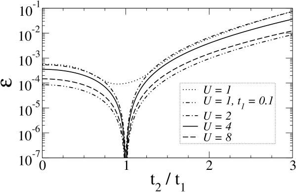
The dependence of errors on fluctuations in the coupling amplitude $t_{2}$ is shown in Fig. 3. Again, the pulse duration used is the optimal value obtained when $t_{2}=t_{1}=0.2$. As expected, the error grows as $t_{2}$ increases. Errors related to large values of $t_{2}$ can also be minimized by increasing the switching time, but the same issues raised above appear.

Figure 4: Comparison of error resulting from a full swap operation and two consecutive square root of swap operations. The error is plotted as a function of upper level detuning in quantum dot $B$. The pulse width is optimized for $\Delta=1$, $t_{1,2}=0.2$, $U=4$, and $\tau=6$. The error for a single square-root-of-swap operation is also shown.

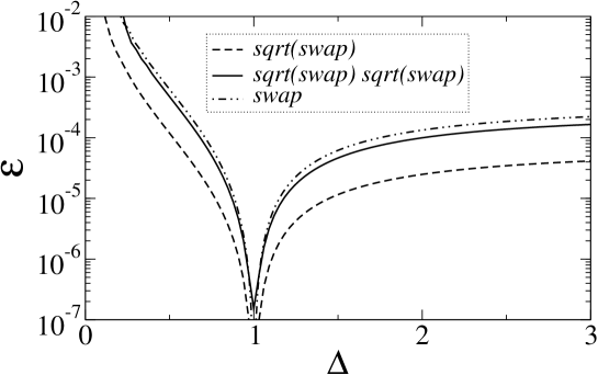
Figure 4 presents the error for two situations involving pulses with duration of about $T/2$, corresponding to the square-root-of-swap operation. The cases shown are: (i) one, and (ii) two consecutive square-root-of-swap pulses. For comparison, the curve corresponding to a full swap pulse is also shown. The error for the square-root-of-swap operation is given by Eq. (6) with $|f\rangle$ replaced by

$$\left|f^{\prime}\right>=\frac{1-i}{2}\left|S_{1}\right>+\frac{1+i}{2}\left|T_{1}\right>.$$ (10)

One can observe from Fig. 4 that error rates are nearly the same after a full swap operation and after two consecutive square root of swap operations. This insensitivity of the error to the pulse duration led us to concentrate our effort on the full swap operations.

Figure 5: Probability of having excessively large full swap errors (percentage) as a function of level spacing detuning. The solid (dashed) line corresponds to $\sigma_{\Gamma_{2}}/\bar{\Gamma}_{2}=0$ ($0.1$) at $U=4$ and $t_{1}=0.2$. The inset shows how the probability varies for a fixed width pulse ($T\approx 90$), but different charging energies $U$, when there is a large level-position detuning: $\sigma_{\Delta}=0.2$, $\sigma_{\Gamma_{2}}=0$ (circles) and moderate level-position and coupling detunings: $\sigma_{\Delta}=0.1$, $\sigma_{\Gamma_{2}}/\bar{\Gamma}_{2}=0.1$ (squares).

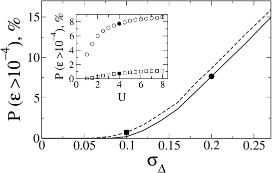
In order to establish an upper bound for QD tuning accuracy, we have performed simulations where both $\Delta$ and $t_{2}$ were allowed to vary. The spacing between the levels in QD $B$ was taken from a Gaussian distribution centered at $\bar{\Delta}=1$, with standard deviation $\sigma_{\Delta}$ ($\epsilon_{N_{B}}^{B}=0$ was kept fixed). For the coupling amplitude, we generated Gaussian distributed level widths $\Gamma_{2}=2\pi\,t_{2}^{2}/\bar{\Delta}$, with average $\bar{\Gamma}_{2}=2\pi\,t_{1}^{2}/\bar{\Delta}$ and standard deviation $\sigma_{\Gamma_{2}}$. The pulses had their widths optimized for the typical case where $\Delta=\bar{\Delta}=1$, $U=4$, $t_{1,2}=0.2$, and $\tau=6$. For fixed values of $\bar{\Delta}$, $\sigma_{\Delta}$, $\bar{\Gamma}_{2}$, and $\sigma_{\Gamma_{2}}$, we generated 10,000 realizations of $\Delta$ and $\Gamma_{2}$ and each time calculated the error after the application of the full swap pulse. In Fig. 5 we show how the probability of having an error larger than the $10^{-4}$ threshold depends on the energy level accuracy, $\sigma_{\Delta}$. Two cases are considered, namely, plain and limited control of the inter-dot coupling constant ($\sigma_{\Gamma_{2}}=0$ and $0.1\,\bar{\Gamma}_{2}$, respectively). The data indicates that frequent, non-correctable errors will happen if an accuracy in $\Delta$ of better than 10 percent is not achieved.

2 Relevance for Real Quantum Dots

To make a quantitative estimate of the impact of these results, let us consider the double QD setup of Jeong and coworkers [87]. In their device, each QD holds about 40 electrons and has a lithographic diameter of 180 nm (we estimate the effective diameter to be around 120 nm, based on the device electron density). The charging energy and mean level spacing of each QD are approximately 1.8 meV and 0.4 meV, respectively (thus $U/\bar{\Delta}\approx 4.5$). If we allow for a maximal inter-dot coupling of $t_{1,2}\approx 0.2\,\bar{\Delta}$ (which yields a level broadening of about $0.25\,\bar{\Delta}$), we find minimal full swap pulse widths of about 100 ps. These values match those used in Fig. 5. For this case, switching times of 10 ps would be long enough to operate in the adiabatic regime and also provide an efficient and well-defined pulse shape. Thus, the combined times should allow for 8-10 consecutive full swap gates before running into dephasing effects related to orbital degrees of freedom [88]. While these numbers are yet too small for large-scale quantum computation, they could be sufficient for the demonstration of QD spin qubits. Based on Fig. 5, we find that accuracies in $\Gamma_{2}$ of about 10% would make operations only limited by dephasing, and not by fluctuation-induced errors. However, as shown in the inset, even for small QDs (typically having small $U/\bar{\Delta}$ ratios), the occurrence of large errors is quite frequent when level detuning is large.

An important issue for multi-electron QDs is their strong mesoscopic, sample-to-sample fluctuations in energy level position and wave-function amplitudes. Our results so far indicate how big an effect a given change in energy or wave-function will produce; now we go further and discuss how mesoscopic fluctuations more generally affect a collection of qubits.

In experiments, several electrodes are placed around the QD surroundings and their voltages are used to adjust the lateral confining potential, the inter-dot coupling, and the coupling between QDs and leads. These voltages are external parameters that can be used to mitigate the effects of mesoscopic fluctuations by tuning energy levels and wave-functions to desired values. Having that in mind, our results indicate two different scenarios for QD qubit implementations.

First, if one is willing to characterize each QD pair separately and have them operate one by one, mesoscopic fluctuations will be irrelevant. It will be possible, with a single parameter per QD, say, to isolate and align energy levels reasonably well. Errors can be further minimized by decreasing the inter-dot coupling (thus increasing $T$). But since QDs are not microscopically identical, each pair of QDs will require a different pulse shape and duration. Multi-electron QDs are tunable enough, easy to couple, and much easier to fabricate than one-electron dots; therefore, multi-electron QDs are most appropriate for this case.

Second, if the goal is to achieve genuine scalability, one has to operate qubits in a similar and uniform way, utilizing a single pulse source. In this case, $T$ and $\tau$ should be the same for all QD pairs. Based on our results above, one should strive to maximally separate the top most occupied state from all other states, occupied or empty, so as to reduce the possibility of leakage during operations with a fixed duration. At the same time, it is important to reduce inter-pair cross-talk induced by capacitive coupling between electrodes, as well as all inter-dot couplings except between the top most states of each QD. One should bear in mind that not all electrodes act independently – in most cases a search in a multidimensional parameter space has to be carried out. Thus, four tuning parameters per QD may be necessary to achieve the following goals: (i) find isolated, single-occupied energy level (two parameters); (ii) align this level with the corresponding level in an adjacent QD (one parameter); (iii) control the inter-dot coupling (one parameter). For parameters involved in (i) and (ii), an accuracy of a few percent will likely be required. Finally, control over the inter-dot coupling parameter, (iii), must allow for the application of smooth pulse shapes in the picosecond range. Our simulations also show that the pulse width must be controlled within at least $0.5\%$ accuracy. Although these requirements seem quite stringent, recent experiments indicate that they could be met [89].

6 Conclusions

In summary, our analysis indicate that mid-size QDs, with ten to a few tens of electrons, while not allowing for extremely fast gates, are still good candidates for spin-qubits. They offer the advantage of being simpler to fabricate and manipulate, but at the same time require accurate, simultaneous control of several parameters. Errors related to detuning and sample-to-sample fluctuations can be large, but can be kept a secondary concern with respect to dephasing effects provided that a sufficient number of independent electrodes or tuning parameters exists.

Chapter 5 Time Evolution of the Reduced Density Matrix

1 Introduction

One of the most fundamental problems in theoretical physics is that of a quantum mechanical system coupled to the bosonic (or fermionic) bath [90, 91]. One such example is presented in the next chapter where we consider double QD charge qubit coupled to the acoustic phonon bath. Formal solution to the problem can be found [see Eqs. (17) and (18) below], nonetheless to do any practical calculation one has to (a) make simplifying assumptions like Born and Markov approximations in the derivation of the Redfield equation [92, 93] or (b) implement sophisticated numerical integration procedure like QUAPI (quasiadiabatic propagator path integral) [94, 95, 96, 97, 98].

Time evolution of the isolated quantum mechanical system is governed by the Schrödinger equation. Therefore, (i) its energy is conserved and (ii) its phase coherence is preserved over time. Coupling to the bath leads to the energy relaxation – decoherence and loss of phase coherence – dephasing. These processes are important for quantum computations because they may potentially destroy the phase coherence of both unentangled single qubit states and especially entangled states of many qubits.

In our treatment of the problem we choose to go along the lines of Born and Markov approximations which eventually lead us to the Redfield equation [92, 93] because (i) we are interested in time evolution of the reduced density matrix at sufficiently long times and (ii) this formalism allows us to obtain analytical expressions for both qubit decoherence and dephasing rates. These analytical expressions contain valuable information about the dependence of the rates on different parameters of the double QD setup.

In this chapter we give formal derivation of the Redfield equation making simplifying assumptions along the way. We employ the projection operator technique [99] as it provides the most transparent way of the derivation.

The plan of this chapter is as follows. In Section 2 we formulate the problem. In Section 3 we find formal solution of the problem. In Section 4 we assume that the quantum mechanical system and the bath are unentangled at $t=0$ and also make Born approximation. Finally, in Section 5 we make Markov approximation and finalize the derivation of the Redfield equation.

2 Formulation of the Problem

The Hamiltonian of the total system is

$$H(t)=H_{S}(t)+H_{B}+V,$$ (1)

where $H_{S}(t)$ is the Hamiltonian of the system, $H_{B}$ is the Hamiltonian of the bath, and $V$ is the Hamiltonian of their interaction. We assume that it can be factorized as follows:

$$V=\sum_{i}K_{i}\Phi_{i},$$ (2)

where $\{K_{i}\}$ are the operators in the system’s of interest Hilbert space and $\{\Phi_{i}\}$ are the operators in the bath Hilbert space. Time evolution of the total system obeys Schrödinger equation for the density matrix:

$$i\frac{d}{dt}\rho(t)=[H(t),\rho(t)].$$ (3)

Our goal is to find similar equation for the time evolution of the reduced (system’s of interest) density matrix $\sigma(t)$.

3 General Solution

Let us write $\rho(t)$ as follows:

$$\rho(t)=f(H_{B})\sigma(t)+\eta(t),$$ (4)

where

$$f(H_{B})=\frac{e^{-\beta H_{B}}}{tr_{b}e^{-\beta H_{B}}}.$$ (5)

One can always do this because no assumption is made about $\eta(t)$. Now let us substitute Eq. (4) into Eq. (3). We obtain

$$i\left[f(H_{B}){\dot{\sigma}}(t)+{\dot{\eta}}\right]=f(H_{B})[H_{S}(t),\sigma(t)]+[H_{S}(t),\eta(t)]$$ (6)

$$+[H_{B},\eta(t)]+[V,f(H_{B})\sigma(t)]+[V,\eta(t)].$$

To find the equation on $\sigma(t)$ let us trace left and right hand sides of Eq. (6) over bath degrees of freedom. The following identities are useful in simplifying the traces:

$$tr_{b}\eta(t)=0,~{}~{}tr_{b}f(H_{B})=1,~{}~{}tr_{b}[Vf(H_{B})]=\sum_{i}K_{i}tr_{b}[\Phi_{i}f(H_{B})]=0.$$ (7)

The last identity should be valid for the most practical applications (it is certainly valid for the phonons coupled to the electric charge, for example). Then the equation for the reduced density matrix becomes

$$i{\dot{\sigma}}(t)=[H_{S}(t),\sigma(t)]+tr_{b}[V,\eta(t)],$$ (8)

where

$$tr_{b}[V,\eta(t)]=\sum_{i}[K_{i},tr_{b}\{\Phi_{i}\eta(t)\}].$$ (9)

However there is one problem: Eq. (8) contains $\eta(t)$ as well. Therefore, one has to find the second (coupled to the first one) equation on $\eta(t)$. This can be done by acting with the projection operator $P=1-f(H_{B})tr_{b}$ on both sides of Eq. (6). A little bit more involved calculation leads to the following result:

$$i{\dot{\eta}}(t)=[H_{S}(t),\eta(t)]+[H_{B},\eta(t)]+[V,\eta(t)]+[V,f(H_{B})\sigma(t)]-f(H_{B})tr_{b}[V,\eta(t)].$$ (10)

One can write Eqs. (8) and (10) in a more compact form as follows:

$${\dot{\sigma}}(t)=-i\,{\mathcal{H}}_{S}(t)\sigma(t)-i\,tr_{b}{\mathcal{V}}\eta(t)$$ (11)

$${\dot{\eta}}(t)=-i\,[{\mathcal{H}}_{S}(t)+{\mathcal{H}}_{B}+P{\mathcal{V}}]\eta(t)-i\,{\mathcal{V}}f(H_{B})\sigma(t),$$ (12)

where ${\mathcal{H}}_{S}$, ${\mathcal{H}}_{B}$, and ${\mathcal{V}}$ are the Liouvillian operators: ${\mathcal{H}}_{S}(t)\sigma(t)=[H_{S}(t),\sigma(t)]$, ${\mathcal{V}}\eta(t)=[V,\eta(t)]$, etc.

Our further plan is as follows. Firstly, let us solve Eq. (12), that is, find the solution for $\eta(t)$ – it is going to have some functional dependence on $\sigma(t)$. Secondly, let us substitute the solution in Eq. (11) and simplify the expression obtained.

Eqs. (11) and (12) have the following form:

$${\dot{\eta}}(t)={\mathcal{A}}(t)\eta(t)+B(t)$$ (13)

$$\eta(0)=\eta_{0}.$$ (14)

This differential equation has a standard solution which can be written as follows

$$\eta(t)={\mathcal{S}}(t,0)\eta_{0}+\int_{0}^{t}dt^{\prime}\,{\mathcal{S}}(t,t^{\prime})B(t^{\prime}),~{}~{}\mbox{where}~{}~{}{\mathcal{S}}(t,t^{\prime})={\hat{T}}e^{\int_{t^{\prime}}^{t}dx\,{\mathcal{A}}(x)}$$ (15)

and ${\hat{T}}$ is a time-ordering operator. How do we understand ${\mathcal{S}}(t,0)\eta_{0}$ term in Eq. (15), for example? It should be understood as follows:

$${\mathcal{S}}(t,0)\eta_{0}={\hat{T}}e^{\int_{0}^{t}dx\,{\mathcal{A}}(x)}\eta_{0}={\hat{T}}e^{\int_{0}^{t}dx\,A(x)}\,\eta_{0}\,{\hat{T}}_{-}e^{-\int_{0}^{t}dx\,A(x)},$$ (16)

where ${\hat{T}}_{-}$ is an anti-time-ordering operator. Eq. (15) solves Eq. (12). Let us substitute the solution in Eq. (11). Thus, we obtain closed form differential equation for $\sigma(t)$:

$${\dot{\sigma}}(t)=-i\,{\mathcal{H}}_{S}(t)\sigma(t)-i\,tr_{b}{\mathcal{V}S}(t,0)\eta_{0}-tr_{b}{\mathcal{V}}\int_{0}^{t}dt^{\prime}{\mathcal{S}}(t,t^{\prime}){\mathcal{V}}f(H_{B})\sigma(t^{\prime}),$$ (17)

where

$${\mathcal{S}}(t,t^{\prime})={\hat{T}}e^{-i\int_{t^{\prime}}^{t}dx[{\mathcal{H}}_{S}(x)+{\mathcal{H}}_{B}+P{\mathcal{V}}]}.$$ (18)

An important note is due at this time. At $t=0$: $\rho(0)=f(H_{B})\sigma_{0}+\eta_{0}$. Therefore, if system and bath are not entangled at $t=0$ then $\eta_{0}=0$ and second term in Eq. (17) simply vanishes.

4 $\eta_{0}=0$ and Born Approximations

Eq. (17) may look simple but it is difficult to solve mainly due to complex structure of the ${\mathcal{S}}$ matrix. Let us make a couple of simplifying assumptions. Firstly, let us assume that $\eta_{0}=0$ then second term in Eq. (17) vanishes. Secondly, let us assume that the system is weakly coupled to the bath ($V$ is small) and keep only the leading term in powers of $V$ expansion of the third term (Born approximation):

$${\mathcal{S}}(t,t^{\prime})={\mathcal{S}}_{0}(t,t^{\prime})+O({\mathcal{V}}),~{}~{}\mbox{where}~{}~{}{\mathcal{S}}_{0}(t,t^{\prime})={\hat{T}}e^{-i\int_{t^{\prime}}^{t}dx[{\mathcal{H}}_{S}(x)+{\mathcal{H}}_{B}]}.$$ (19)

Thus, in $\eta_{0}=0$ and Born approximations, Eq. (17) becomes

$${\dot{\sigma}}(t)=-i\,{\mathcal{H}}_{S}(t)\sigma(t)-tr_{b}{\mathcal{V}}\int_{0}^{t}dt^{\prime}{\mathcal{S}}_{0}(t,t^{\prime}){\mathcal{V}}f(H_{B})\sigma(t^{\prime}),$$ (20)

where the first term on the right hand side is the conventional Liouvillian term corresponding to the time reversible dynamics and the second term is a dissipative term (or time irreversible part).

The dissipative term can be further simplified. First, let us simplify ${\mathcal{S}}_{0}$:

$${\mathcal{S}}_{0}(t,t^{\prime})={\mathcal{S}}_{S}(t,t^{\prime})e^{-i(t-t^{\prime}){\mathcal{H}}_{B}},~{}~{}\mbox{where}~{}~{}{\mathcal{S}}_{S}(t,t^{\prime})={\hat{T}}e^{-i\int_{t^{\prime}}^{t}dx{\mathcal{H}}_{S}(x)}.$$ (21)

Then, the dissipative term becomes

$$-\int_{0}^{t}dt^{\prime}\,tr_{b}\left[V,{\mathcal{S}}_{S}(t,t^{\prime})\left[e^{-i(t-t^{\prime})H_{B}}Ve^{i(t-t^{\prime})H_{B}},f(H_{B})\sigma(t^{\prime})\right]\right].$$ (22)

Further calculations should be performed in the following order: (i) substitute $V=\sum_{i}K_{i}\Phi_{i}$; (ii) take advantage of $tr_{b}$ – define bath correlation functions:

$$B_{ij}(t)=tr_{b}\left[\Phi_{i}(t)\Phi_{j}f(H_{b})\right],$$ (23)

$$B_{ij}(-t)=tr_{b}\left[\Phi_{i}\Phi_{j}(t)f(H_{b})\right],$$ (24)

$$\left[B_{ji}(-t)\right]^{\dagger}=B_{ij}(t);$$ (25)

(iii) to transform $\sigma(t-y)$ to $\sigma(t)$ use:

$${\mathcal{S}}_{S}(t,t-y)\,\sigma(t-y)=\sigma(t)+O({\mathcal{V}}^{2}).$$ (26)

The final form of the equation for the time evolution of the reduced density matrix in $\eta_{0}=0$ and Born approximations is

$${\dot{\sigma}}(t)=-i\left[H_{S}(t),\sigma(t)\right]+\sum_{j}\left[\Lambda_{j}(t)\,\sigma(t),K_{j}\right]+\mbox{H.c.},$$ (27)

where

$$\Lambda_{j}(t) = \sum_{i}\int_{0}^{t}dy\,B_{ji}(y)\,{\mathcal{S}}_{S}(t,t-y)\,K_{i}$$ (28)

$$= \sum_{i}\int_{0}^{t}dy\,B_{ji}(y)\,{\hat{T}}e^{-i\int_{t-y}^{t}dx\,H_{S}(x)}\,K_{i}\,{\hat{T}}_{-}e^{i\int_{t-y}^{t}dx\,H_{S}(x)}.$$ (29)

The structure of $\Lambda$-matrices is quite complex. Moreover, at each time slice in the integration of Eq. (27) one has to numerically calculate $\Lambda$-matrices all over again.

5 Markov Approximation on Top: Redfield Equation

One conventional way to simplify Eq. (29) and make Eq. (27) local in time is to assume that bath has no memory. That is, bath correlation time $\tau_{c}$ is the smallest time scale in the problem. This is called Markov approximation. In this approximation one can only find evolution of the system at sufficiently long times: $t>\tau_{c}$. Since $B_{ji}(y)\to 0$ for $y>\tau_{c}$, only small values of $y$ contribute in Eq. (29). Hence,

$$\int_{t-y}^{t}dx\,H_{S}(x)\approx y\,H_{S}(t)$$ (30)

and upper limit of the integration over $y$ in Eq. (29) can be extended to $\infty$. Thus, $\Lambda$-matrices in Born-Markov approximation can be written as follows:

$$\Lambda_{j}(t)=\sum_{i}\int_{0}^{\infty}dy\,B_{ji}(y)\,e^{-iyH_{S}(t)}\,K_{i}\,e^{iyH_{S}(t)}.$$ (31)

Eq. (27) with $\Lambda$-matrices given by Eq. (31) is local in time and called Redfield equation [92, 93, 99, 100].

Chapter 6 Phonon Decoherence of a Double Quantum Dot Charge Qubit

1 Overview

In this chapter we study decoherence of a quantum dot charge qubit due to coupling to piezoelectric acoustic phonons in the Born-Markov approximation. After including appropriate form factors, we find that phonon decoherence rates are one to two orders of magnitude weaker than was previously predicted. We calculate the dependence of the $Q$-factor on lattice temperature, quantum dot size, and interdot coupling. Our results suggest that mechanisms other than phonon decoherence play a more significant role in current experimental setups.

The work in this chapter was done in collaboration with Eduardo R. Mucciolo and Harold U. Baranger.

2 Introduction

Since the discovery that quantum algorithms can solve certain computational problems much more efficiently than classical ones [101], attention has been devoted to the physical implementation of quantum computation. Among the many proposals, there are those based on the electron spin [55, 69] or charge [102, 103, 104, 105, 81, 106] in laterally confined quantum dots, which may have great potential for scalability and integration within current technologies.

Single qubit operations involving the spin of an electron in a quantum dot will likely require precise engineering of the underlying material or control over local magnetic fields [62]; both have yet to be achieved in practice. In contrast, single qubit operations involving charge in a double quantum dot (DQD) [107] are already within experimental reach [88, 108, 109]. They can be performed either by sending electrical pulses to modulate the potential barrier between the dots (tunnel pulsing) [104, 105, 106] or by changing the relative position of the energy levels (bias pulsing) [88, 108]. In both cases one acts on the overlap between the electronic wave functions of the dots. This permits direct control over the two low-energy charge states of the system – the basis states $|1\rangle$ and $|2\rangle$ of a qubit: Calling $N_{1}$ ($N_{2}$) the number of excess electrons in the left (right) dot, we have that $|1\rangle=(1,0)$ and $|2\rangle=(0,1)$.

Figure 1: Schematic Coulomb blockade stability diagram for a double quantum dot system at zero bias [107]. $(N_{1},N_{2})$ denotes the number of excess electrons in the dots for given values of the gate voltages $V_{1}$ and $V_{2}$. The solid lines indicate transitions in the total charge, while the dotted lines indicate transitions where charge only moves between dots. The point $A$ marks the qubit working point.

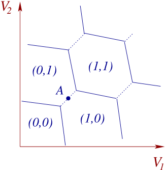
The proposed DQD charge qubit relies on having two lateral quantum dots tuned to the $(1,0)\!\leftrightarrow\!(0,1)$ transition line of the Coulomb blockade stability diagram (see Fig. 1). Along this line, an electron can move between the dots with no charging energy cost. An advantage of this system is that the Hilbert space is two-dimensional, even at moderate temperatures, since single-particle excitations do not alter the charge configuration. Leakage from the computational space involves energies of order the charging energy which is quite large in practice ($\sim\!1$ meV $\sim\!10$ K). In the case of tunnel pulsing, working adiabatically – such that the inverse of the switching time is much less than the charging energy – assures minimal leakage. The large charging energy implies that pulses as short as tens to hundreds of picoseconds would be well within the adiabatic regime. However, the drawback of using charge to build qubits is the high decoherence rates when compared to spin. Since for any successful qubit one must be able to perform single- and double-qubit operations much faster than the decoherence time, a quantitative understanding of decoherence mechanisms in a DQD is essential.

In this chapter, we carry out an analysis of phonon decoherence in a DQD charge qubit. During qubit operations, the electron charge movement induces phonon creation and annihilation, thus leading to energy relaxation and decoherence. In order to quantify these effects, we follow the time dependence of the system’s reduced density matrix, after tracing out the phonon bath, using the Redfield formalism in the Born and Markov approximations [99, 100].

Our results show that decoherence rates for this situation are one to two orders of magnitude weaker than previously estimated. The discrepancy arises mainly due to the use of different spectral functions. Our model incorporates realistic geometric features which were lacking in previous calculations. When compared to recent experimental results, our calculations indicate that phonons are likely not the main source of decoherence in current DQD setups.

The chapter is organized as follows. In Section 3, we introduce the model used to describe the DQD, discuss the coupling to phonons, and establish the Markov formulation used to solve for the reduced density matrix. In Section 4 we study decoherence in a single-qubit operation, while in Section 5 we simulate the bias pulsing experiment of Refs. [88, 108]. Finally, in Section 6 we present our conclusions.

3 Model System

We begin by assuming that the DQD is isolated from the leads. The DQD and the phonon bath combined can then be described by the total Hamiltonian [81]

$$H=H_{S}+H_{B}+H_{SB},$$ (1)

where $H_{S}$ and $H_{B}$ are individual DQD and phonon Hamiltonians, respectively, and $H_{SB}$ is the electron-phonon interaction. We assume that gate voltages are tuned to bring the system near the degeneracy point $A$ (Fig. 1) where a single electron may move between the two dots with little charging energy cost. To simplify the presentation, only one quantum level on each dot is included; $E_{1(2)}$ denotes the energy of an excess electron on the left (right) QD (possibly including some charging energy). Likewise, spin effects are neglected. Thus, in the basis $\{\left|1\right>$, $\left|2\right>\}$, the DQD Hamiltonian reads

$$H_{S}=\frac{\varepsilon(t)}{2}\,\sigma_{z}+v(t)\,\sigma_{x},$$ (2)

where $\sigma_{z,x}$ are Pauli matrices, $\varepsilon(t)\!=\!E_{1}\!-\!E_{2}$ is the energy level difference, and $v(t)$ is the tunneling amplitude connecting the dots. Notice that both $\varepsilon$ and $v$ may be time dependent. The phonon bath Hamiltonian has the usual form ($\hbar=1$)

$$H_{B}=\sum_{\bf q}\omega_{\bf q}\,b^{\dagger}_{\bf q}b_{\bf q},$$ (3)

where the dispersion relation $\omega_{\bf q}$ is specified below. The electron-phonon interaction has the linear coupling form [81, 110],

$$H_{SB}=\sum_{\bf q}\sum_{i=1}^{2}\alpha_{\bf q}^{(i)}\,N_{i}\,\left(b_{\bf q}^{\dagger}+b_{-{\bf q}}\right),$$ (4)

where $N_{i}$ is the number of excess electrons in the $i$-th dot and $\alpha_{\bf q}^{(i)}=\lambda_{\bf q}\,e^{-i{\bf q}\cdot{\bf R}_{i}}\,P_{i}({\bf q})$, with ${\bf R}_{1}\!=\!0$ and ${\bf R}_{2}\!=\!{\bf d}$ the dot position vectors, see Fig. 2. The dependence of the coupling constant $\lambda_{\bf q}$ on the material parameters and on the wave vector ${\bf q}$ will be specified below. The dot form factor is

Figure 2: Geometry of the double quantum dot charge qubit.

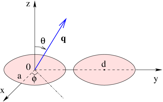
$$P_{i}({\bf q})=\int d^{3}r\,n_{i}({\bf r})\,e^{-i{\bf q}\cdot{\bf r}},$$ (5)

where $n_{i}({\bf r})$ is the excess charge density in the $i$-th dot. With no significant loss of generality, we will assume that the form factor is identical for both dots and, therefore, drop the $i$ index hereafter. In the basis $\{\left|1\right>$, $\left|2\right>\}$, after dropping irrelevant constant terms, the electron-phonon interaction simplifies to

$$H_{SB}=K\,\Phi,$$ (6)

where

$$K=\frac{1}{2}\,\sigma_{z}\qquad\mbox{and}\qquad\Phi=\sum_{\bf q}g_{\bf q}\,\left(b^{\dagger}_{\bf q}+b_{-\bf q}\right),$$ (7)

with $g_{\bf q}\!=\!\lambda_{\bf q}\,P({\bf q})\,\left(1-e^{-i{\bf q}\cdot{\bf d}}\right)$. The phonons propagate in three dimensions, while the electrons are confined to the plane of the underlying two-dimensional electron gas (2DEG). Notice that the electron-phonon coupling is not isotropic for the DQD (Fig. 2): Phonons propagating along $\phi\!=\!0$ and any $\theta$ do not cause any relaxation, while coupling is maximal along $\phi\!=\!\theta\!=\!\pi/2$ direction. We neglect any mismatch in phonon velocities at the GaAs/AlGaAs interface, where the 2DEG is located.

We now proceed with the Born-Markov-Redfield treatment of this system, see Chapter 5. While the Born approximation is clearly justified for weak electron-phonon interaction, the Markov approximation requires, in addition, that the bath correlation time is the smallest time scale in the problem. These conditions are reasonably satisfied for lateral GaAs quantum dots, as we will argue below.

Let us assume that the system and the phonon bath are disentangled at $t=0$. Using Eqs. (2), (3), and (6), we can write the Redfield equation for the reduced density matrix $\rho(t)$ of the DQD (see Chapter 5),

$${\dot{\rho}(t)}=-i\left[H_{S}(t),\rho(t)\right]+\left\{\left[\Lambda(t)\rho(t),K\right]+\mbox{H.c.}\right\}\;.$$ (8)

The first term on the right-hand side yields the Liouvillian evolution and the other terms yield the relaxation caused by the phonon bath. The auxiliary matrix $\Lambda$ is defined as

$$\Lambda(t)=\int_{0}^{\infty}d\tau\,B(\tau)\,e^{-i\tau H_{S}(t)}\,K\,e^{i\tau H_{S}(t)}$$ (9)

where $B(\tau)\!=\!{\rm Tr}_{b}\{\Phi(\tau)\Phi(0)f(H_{B})\}$ is the bath correlation function, $\Phi(\tau)\!=\!e^{iH_{B}\tau}\,\Phi\,e^{-iH_{B}\tau}$, and $f(H_{B})\!=\!e^{-\beta H_{B}}/{\rm Tr}_{b}\{e^{-\beta H_{B}}\}$, with $\beta\!=\!1/T$ the inverse lattice temperature ($k_{B}=1$).

Using Eq. (3) in the definition of the bath correlation function, we find that the latter can be expressed in the form

$$B(\tau)=\int_{0}^{\infty}\!\!d\omega\,\nu(\omega)\,\{e^{i\tau\omega}n_{B}(\omega)+e^{-i\tau\omega}[1+n_{B}(\omega)]\},$$ (10)

where $n_{B}(\omega)$ is the Bose-Einstein distribution function and

$$\nu(\omega)=\sum_{\bf q}|g_{\bf q}|^{2}\,\delta(\omega-\omega_{\bf q})$$ (11)

is the spectral density of the phonon bath.

We now specialize to linear, isotropic acoustic phonons: $\omega_{\bf q}\!=\!s|{\bf q}|$, where $s$ is the phonon velocity. Moreover, we only consider coupling to longitudinal piezoelectric phonons, neglecting the deformation potential contribution. For bulk GaAs, this is justifiable at temperatures below approximately 10 $K$ (see Appendix 9). Thus,

$$|\lambda_{\bf q}|^{2}=\frac{g_{\rm ph}\,\pi^{2}s^{2}}{\Omega|{\bf q}|},$$ (12)

where $g_{\rm ph}$ is the piezoelectric constant in dimensionless form ($g_{\rm ph}\!\approx\!0.05$ for GaAs [110, 111]) and $\Omega$ is the unit cell volume.

The excess charge distribution in the dots is assumed Gaussian:

$$n({\bf r})=\delta(z)\,\frac{1}{2\pi a^{2}}\exp\left(-\frac{x^{2}+y^{2}}{2a^{2}}\right).$$ (13)

This is certainly a good approximation for small dots with few electrons, but becomes less accurate for large dots. The resulting form factor reads

$$P({\bf q})=e^{-(q_{x}^{2}+q_{y}^{2})a^{2}/2}.$$ (14)

Note that this expression differs from that in Refs. [104, 105, 106] where a three-dimensional Gaussian charge density was assumed.

Using Eqs. (12) and (14), as well as the DQD geometry of Fig. 2, we get

$$\nu(\omega)=g_{\rm ph}\omega\int_{0}^{\pi/2}d\theta\sin\theta\exp\left(-\frac{\omega^{2}a^{2}}{s^{2}}\sin^{2}\theta\right)\left[1-J_{0}\left(\frac{\omega d}{s}\sin\theta\right)\right].$$ (15)

It is instructive to inspect the asymptotic limits of this equation. At low frequencies, $\nu(\omega\rightarrow 0)\!\approx\!g_{\rm ph}\,d^{2}\,\omega^{3}/6s^{2}$; thus, the phonon bath is superohmic. At high frequencies,

$$\nu(\omega\rightarrow\infty)\approx\frac{g_{\rm ph}\,s^{2}}{a^{2}\omega}f\left(\frac{d}{a}\right),$$ (16)

where

$$f\left(\frac{d}{a}\right)=\int_{0}^{\infty}dx~{}x~{}e^{-x^{2}}\left[1-J_{0}\left(\frac{d}{a}x\right)\right].$$ (17)

Notice that the spectral function does not have the exponential decay familiar from the spin-boson model, but rather falls off much more slowly: $\nu(\omega\!\rightarrow\!\infty)\!\propto\!\omega^{-1}$. This should be contrasted with the phenomenological expressions used in Ref. [81].

The characteristic frequency of the maximum in $\nu(\omega)$ is $\tau_{c}^{-1}=s/a$. For typical experimental setups, $a\!\approx\!50$ nm while $s\!\approx\!5\times 10^{3}$ m/s for GaAs, yielding $\tau_{c}\!\approx\!10$ ps ($\tau_{c}^{-1}\!\approx\!65\,\mu$eV). Thus, the Markovian approximation can be justified for time scales $t>\tau_{c}$ and if all pulse operations are kept adiabatic on the scale of $\tau_{c}$.

4 Decay of Charge Oscillations

One can operate this charge qubit in two different ways: (i) by pulsing the tunneling amplitude $v(t)$ keeping $\varepsilon$ constant, or (ii) by changing the energy level difference $\varepsilon(t)$ keeping $v$ constant (bias pulsing). Tunnel pulsing seems advantageous as it implies fewer decoherence channels and less leakage. However, a recent experiment used a bias pulsing scheme [88, 108].

Our system’s Hilbert space is two-dimensional by construction [see Eq. (2)], hence there is no leakage to states outside the computational basis. We can, therefore, use square pulses instead of smooth, adiabatic ones. This not only allows us to analytically solve for the time evolution of the reduced density matrix, Eq. (8), but also renders our results applicable to both tunnel and bias pulsing. Indeed, in both regimes one has $\varepsilon(t)\!=\!0$ and $v(t)\!=\!v_{m}$ for $t>0$, taking that the pulse starts at $t=0$. Let us assume that the excess electron is initially in the left dot: $\rho_{11}(0)\!=\!1$ and $\rho_{12}(0)\!=\!0$. In this case, since the coefficients on the right-hand side of (8) are all constants at $t>0$, we can solve the Redfield equation exactly (see Appendix 10 for details). As $\rho(t)$ has only three real independent components, the solution is

$$\rho_{11}(t) = \frac{1}{2}+\frac{1}{2}e^{-\frac{\gamma_{1}}{2}t}(\cos\omega t+\frac{\gamma_{1}}{2\omega}\sin\omega t),$$ (18)

$$\mbox{Re}\,\rho_{12}(t) = -\frac{1}{2}(1-e^{-\gamma_{1}t})\tanh\frac{v_{m}}{T},$$ (19)

$$\mbox{Im}\,\rho_{12}(t) = \frac{2v_{m}+\gamma_{2}}{2\omega}\,e^{-\frac{\gamma_{1}}{2}t}\sin\omega t,$$ (20)

where

$$\omega = \left[4v_{m}\left(v_{m}+\frac{\gamma_{2}}{2}\right)-\frac{\gamma_{1}^{2}}{4}\right]^{1/2},$$ (21)

$$\gamma_{1} = \frac{\pi}{2}\,\nu(2v_{m})\coth\frac{v_{m}}{T},$$ (22)

$$\gamma_{2} = -\,\mathchoice{{\vbox{\hbox{$\textstyle-$}}\kern-4.86108pt}}{{\vbox{\hbox{$\scriptstyle-$}}\kern-3.25pt}}{{\vbox{\hbox{$\scriptscriptstyle-$}}\kern-2.29166pt}}{{\vbox{\hbox{$\scriptscriptstyle-$}}\kern-1.875pt}}\!\int_{0}^{\infty}\frac{dy}{y^{2}-1}\nu(2v_{m}y)\coth\frac{v_{m}y}{T}.$$ (23)

Note that $\gamma_{1,2}\!\ll\!v_{m}$. We extract the customary energy and phase relaxation times, $T_{1}$ and $T_{2}$, by rotating to the energy eigenbasis $\{\left|-\right>$, $\left|+\right>\}$:

$$\rho_{--}(t) = \frac{1}{2}-\mbox{Re}\,\rho_{12}(t),$$ (24)

$$\rho_{-+}(t) = -\frac{1}{2}+\rho_{11}(t)+i\,\mbox{Im}\,\rho_{12}(t).$$ (25)

Then, the damping of the oscillations in the diagonal matrix elements is the signature of energy relaxation, while the phonon-induced decoherence is seen in the exponential decay of the off-diagonal elements. For the DQD, we find $T_{1}\!=\!\gamma_{1}^{-1}$ and $T_{2}\!=\!2\gamma_{1}^{-1}$ for the decoherence time.

The quality factor of the charge oscillations in Eq. (18) is $Q=\omega/\pi\gamma_{1}$. Using Eqs. (21), (22), and (15), we find that

$$Q\approx\frac{4\tanh(v_{m}/T)}{\pi^{2}g_{\rm ph}}\,\left\{\int_{0}^{1}\frac{dx}{\sqrt{1-x}}\,e^{-(v_{m}/\omega_{a})^{2}\,x}\left[1-J_{0}\left(\frac{d}{a}\frac{v_{m}}{\omega_{a}}\sqrt{x}\right)\right]\right\}^{-1},$$ (26)

where $\omega_{a}=s/2a$. The $Q$-factor depends on the tunneling amplitude $v_{m}$, lattice temperature $T$, dot radius $a$, and interdot distance $d$.

Several experimental realizations of DQD systems recently appeared in the literature [88, 108, 109, 87, 89]. In principle, all these setups could be driven by tunnel pulsing to manipulate charge and perform single-qubit operations. To understand how the $Q$-factor depends on the tunneling amplitude $v_{m}$ in realistic conditions, let us consider the DQD setup of Jeong and coworkers [87]. In their device, each dot holds about 40 electrons and has a lithographic diameter of 180 nm. The effective radius $a$ is estimated to be around 60 nm based on the device electron density. Therefore, $d/a\!\approx\!3$. The lattice base temperature is 15 mK. Introducing these parameters into Eq. (26), one can plot $Q$-factor as a function of $v_{m}$ or, equivalently, as a function of the period of the charge oscillations $P=2\pi/\omega\!\approx\!\pi/v_{m}$. This is shown in Fig. 3.

Figure 3: The charge oscillation $Q$-factor as a function of the tunneling amplitude $v_{m}$ (lower scale) and of the oscillation period $P$ (upper scale) for a GaAs double quantum dot system. The lattice temperature is $15$ mK and the dot radius and interdot distance are 60 nm and 180 nm, respectively. The inset shows the relation between $P$ and $Q$ at small tunneling amplitudes (large periods).

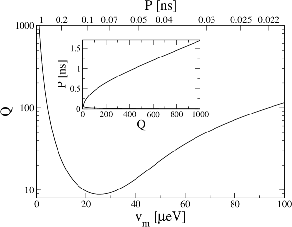
To stay in the tunnel regime $v_{m}$ should be smaller than the mean level spacing of each QD, approximately 400 $\mu$eV in the experiment [87]. Therefore, in Fig. 3 we only show the curve for $v_{m}$ up to 100 $\mu$eV. One has to recall that at these values the Markov approximation used in the Redfield formulation is not accurate (see end of Section 3), and so our results are only an estimate for $Q$. For strong tunneling amplitudes, when $25\,\mu{\rm eV}<v_{m}<100\,\mu{\rm eV}$, the largest value we find for $Q$ is close to 100. For weak tunneling with $v_{m}<25\,\mu{\rm eV}$, the situation is more favorable and larger quality factors (thus relatively less decoherence) can be achieved. Nevertheless, the one-qubit operation time, which is proportional to the period, grows linearly with $Q$ in the region of $v_{m}\to 0$, as shown in the inset of Fig. 3. Therefore, at a certain point other decoherence mechanisms are going to impose an upper bound on $Q$.

Figure 4: The charge oscillation $Q$-factor as a function of the lattice temperature. Inset: as a function of the dot radius for a fixed ratio $d/a=3$. The solid (dashed) line corresponds to the weak $v_{m}\!\simeq\!53$ mK (strong $v_{m}\!\simeq\!1.1$ K) tunneling regime. Other parameter values are equal to those in Fig. 3.

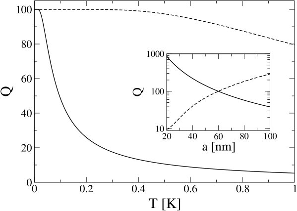
The minimum of $Q$ in Fig. 3 occurs when $v_{m}$ coincides with the frequency at which the phonon spectral density is maximum. It corresponds to the energy splitting between bonding and anti-bonding states of the DQD, $2v_{m}$, being approximately equal to the frequency of the strongest phonon mode $s/a$: $v_{m}\simeq\omega_{a}$.

From Fig. 3, it is evident that one can reach certain values for the $Q$-factor (say, $Q=100$) at both weak ($v_{m}\simeq 4.6~{}\mu$eV $\simeq 53$ mK) and strong ($v_{m}\simeq 93~{}\mu$eV $\simeq 1.1$ K) tunneling. However, these two regimes are not equally convenient. From Eq. (26), it is clear that the temperature dependence of the $Q$-factor is fully determined by the bonding-antibonding splitting energy $2v_{m}$: $Q(T)\!=\!Q(0)\tanh(v_{m}/T)$. We notice that $Q(T)\!\approx\!Q(0)$ if $T\ll v_{m}$; therefore, the $Q$-factor is less susceptible to temperature variations for strong tunneling (Fig. 4). Another parameter that influences the $Q$-factor is the dot radius, which controls the frequency of the strongest phonon mode, $s/a$. In the strong tunneling regime (dashed curve in the inset to Fig. 4), one has to increase the QD size to improve the $Q$-factor. This would reduce the energy level spacing, hence only moderate improvement in $Q$-factor is possible. In contrast, in the weak tunneling regime (solid curve in the inset to Fig. 4) one has to reduce the QD size. This can lead to a significant (up to one order of magnitude) $Q$-factor improvement.

5 Bias Pulsing

In a recent experiment [88, 108], Hayashi and coworkers studied charge oscillations in a bias-pulsed DQD. In this regime the energy difference between the left and right-dot single-particle energy levels is a function of time: $\varepsilon(t)=\varepsilon_{0}\,u(t)$. A typical profile used for pulsing is

$$u(t)=1-\frac{1}{2}\left(\tanh\frac{t+W/2}{2\tau}-\tanh\frac{t-W/2}{2\tau}\right),$$ (27)

where $W$ represents the pulse width and $\tau$ controls the rise and drop times. During bias pulsing, the tunneling amplitude is kept constant. In Refs. [88, 108], the difference in energy levels was induced by applying a bias voltage between left and right leads (and not by gating the dots separately). For their setup, the maximum level splitting amplitude was $\varepsilon_{0}\!\approx\!30\,\mu{\rm eV}$ and $\tau\!\approx\!15\,{\rm ps}$, corresponding to an effective ramping time of about 100 ps. The tunneling amplitude was kept constant and estimated as $v\!\approx\!5\,\mu{\rm eV}$, which amounts to charge oscillations with period $P\!\approx\!1\,{\rm ns}$. The lattice temperature was $20\,{\rm mK}$. Each quantum dot contained about 25 electrons and the effective dot radius is estimated to be around $50\,{\rm nm}$ based on the device electron density. From the electron micrograph of the device one finds $d\!\approx\!225\,{\rm nm}$, hence $d/a\!\approx\!4.5$. When substituting these values into Eq. (26), one finds $Q\!\approx\!54$.

However, from the experimental data one observes $Q\!\approx\!3$. Low $Q$-factors were also obtained by Petta and coworkers in an experiment where coherent charge oscillations in a DQD were detected upon exciting the system with microwave radiation [109]. Other mechanisms of decoherence do exist in these systems, such as background charge fluctuations [113] and electromagnetic noise emerging from the gate voltages. Our results combined with the recent experiments indicate that these other mechanisms are more relevant than phonons.

We now turn to yet another possible source of decoherence: Leakage to the leads when the pulse is on. To illustrate this alternative source of damping of charge oscillations, we simulate the bias-pulsing experiment of Refs. [88, 108] by implementing a rate equation formalism similar to that used in Ref. [112]. The formalism is based on a transport theory put forward for the strongly biased limit [115, 116]. First, we find the stationary current $I_{0}$ through the DQD structure when the pulse is off (that is, the bias is applied) [116]:

$$I_{0}=e~{}\frac{\Gamma_{L}\Gamma_{R}}{\Gamma_{L}+\Gamma_{R}}~{}\frac{v^{2}}{v^{2}+\frac{\Gamma_{L}\Gamma_{R}}{4}+\frac{\varepsilon_{0}^{2}\Gamma_{L}\Gamma_{R}}{(\Gamma_{L}+\Gamma_{R})^{2}}},$$ (28)

where $e$ is the elementary charge. $\Gamma_{L(R)}$ is the partial width of the energy level in the left (right) dot due to coupling to the left (right) lead (when the bias is applied); in the experiment [88, 108], $\Gamma_{L,R}\!\approx\!30\,\mu{\rm eV}$. On the other hand, when the pulse is on, the stationary current is zero. We now apply the pulse $\varepsilon(t)$ and measure the current $I(t)$. In the experiments, the level widths $\Gamma_{L,R}$ decrease upon biasing the system. To include that effect here, we also pulse them: $\Gamma_{L}(t)\!=\!\gamma_{L}+(\Gamma_{L}-\gamma_{L})u(t)$ and analogously for $\Gamma_{R}$, where $\gamma_{L(R)}$ is the residual leakage to the left (right) lead when the pulse is on. We use $\gamma_{L,R}\!=\!0.3\,\mu{\rm eV}$, even though the real leakage in the experiment was likely much smaller. To obtain the response current one subtracts the stationary component: $I_{\rm resp}(t)\!=\!I(t)-I_{0}u(t)$.

Figure 5: (a) The response current $I_{\rm resp}(t)/e$ in ns^-1 as a function of time for a pulse with $W\!=\!4$ ns and $\tau\!=\!30$ ps. (b) Number of electrons transfered between left and right leads, as defined in Eq. (29), as a function of the pulse width $W$.

Figure 5(a) shows the response current for a pulse of width $W\!=\!4$ ns and $\tau\!=\!30$ ps. The latter is approximately twice as large as in the experiment and is chosen to enhance the effect. In Refs. [88, 108], pulses were applied at a frequency $f\!=\!100$ MHz. The average number of electrons transfered from the left to the right lead per cycle minus that in the stationary regime is [112]

$$n=\int_{0}^{1/f}\!dt\;I_{\rm resp}(t)/e.$$ (29)

(In the simulations there is no need to apply a sequence of pulses.) Notice that $n$ oscillates as a function of the pulse width $W$ [see Fig. 5(b)] as observed in the experiment. Two main conclusions can be drawn from our simulation. First, the larger $\tau$, the smaller the visibility of the charge oscillations [112]. Second, the larger the leakage rates $\gamma_{L,R}$ when the pulse is on, the stronger the damping of the oscillations. While the damping due to leakage is presumably too weak an effect to discern in the data presented in Refs. [88, 108], the loss of visibility due to finite $\tau$ is likely one of the causes of the small amplitude seen experimentally.

6 Conclusions

The main conclusion of the chapter is that, under realistic conditions, phonon decoherence is one to two orders of magnitude weaker than expected [81, 104, 105, 106]. The analytical expression for the $Q$-factor given in Eq. (26) was found using an expression for the phonon spectral density, Eq. (15), which takes into account important information concerning the geometry of the double quantum dot system. In a previous work [81] an approximate, phenomenological expression, $\nu(\omega)\propto\omega\exp(-\omega/\omega_{c})$, was utilized in the treatment of charge qubits. There is a striking difference between these two expressions in both the high- and low-frequency limits. Moreover, an arbitrary coupling constant was adopted in Ref. [81] to model the electron-phonon interaction while our treatment uses a value known to describe the most relevant phonon coupling in GaAs. On the other hand, other previous work [104, 105, 106] assumed a spherically symmetric excess charge distribution in the dot while we have assumed a two-dimensional pancake form. These differences account for most of the discrepancy between the present and previous results.

Based on these findings we conclude that phonon decoherence is too weak to explain the damping of the charge oscillations seen in recent experiments [88, 108, 109]. Charge leakage to the leads during bias pulsing is an additional source of damping, as shown in Fig. 5(b); however, for realistic parameters [88, 108, 112], it turns out to be a weak effect as well. Hence, other decoherence mechanisms, such as background charge fluctuations or noise in the gate voltages, play the dominant role [113].

There are two distinct ways to operate a double quantum dot charge qubit: (i) by tunnel pulsing or (ii) by bias pulsing. Tunnel pulsing seems advantageous due to the smaller number of possible decoherence channels. In addition, the bias pulsing scheme, in contrast to tunnel pulsing, introduces significant loss of visibility in the charge oscillations.

In this chapter we did not attempt to study leakage or loss of fidelity due to non-adiabatic pulsing, which are both important issues for spin-based quantum dot qubits (see Chapter 4). Moreover, we have not attempted to go beyond the Markov approximation when deriving an equation of motion for the reduced density matrix. Both of these restrictions in our treatment impose some limitations on the accuracy of our results, especially for large tunneling amplitudes.

Finally, it is worth mentioning that some extra insight would be gained by measuring the $Q$-factor as a function of the tunneling amplitude $v_{m}$ experimentally. Such a measurement would allow one to map the spectral density of the boson modes responsible for the decoherence. This would provide very valuable information about the leading decoherence mechanisms in double quantum dot systems.

Chapter 7 Conclusion

1 General Overview

The continuous minituarization of the integrated circuits is going to affect the underlying physics of the future computers. This new physics first came into play as the effect of Coulomb blockade in the electron transport through the small conducting island. Then, as the size of the island $L$ continued to shrink further, quantum phase coherence length $L_{\phi}$ became larger than $L$ leading to the mesoscopic fluctuations – fluctuations of the island’s quantum mechanical properties upon small external perturbations. Quantum coherence of the mesoscopic systems is essential for building reliable quantum computer. Unfortunately, one can not completely isolate the system from the environment and its coupling to the environment inevitably leads to the loss of coherence or decoherence. All these effects are to be thoroughly investigated as the potential of the future applications is enormous.

2 Main Conclusions of My Work

In Chapter 1  I studied Coulomb blockade oscillations of the linear conductance through a quantum dot weakly coupled to the leads via multichannel tunnel junctions. To obtain analytic results I have assumed that the energy levels in the QD are equally spaced. The electron-electron interactions in the QD have been described by the constant interaction model, though thermal excitations with all possible spins were taken into account.

Firstly, I found the expression for the linear conductance in the spinless case [Eq. (22)]. It is valid at arbitrary values of $E_{C}$, $\delta E$ and $T$. Then, in Section 5, I applied the spinless case theory result to the problem of the transport via quantum dot in the quantum Hall regime. The quantum dot energy levels in this case are equidistant with the spacing given by Eq. (35).

Linear conductance in the case of spin-$\frac{1}{2}$ electrons at arbitrary values of $E_{C}$, $\delta E$, and $T$ is given by Eq. (58). It is plotted in Fig. 9 for the charging energy of the quantum dot equal to mean level spacing. Eq. (58) can be used as an experimental data fit to extract the charging energy and mean level spacing at given temperature.

Though I do not expect my quantitative results to precisely describe a quantum dot with random energy levels, they certainly give correct order of magnitude for the conductance oscillations and their generic features.

In Chapter 2  I studied corrections to the spacings between Coulomb blockade peaks due to finite dot-lead tunnel couplings. I considered both GUE and GOE random matrix ensembles of 2D quantum dots. The electron-electron interactions in the QD were described by the constant exchange interaction model. $S=0$, $\frac{1}{2}$, and $1$ spin states of the QD were accounted for, thus, limiting the applicability of my results to not so large exchange interaction constants: $J_{\rm s}<0.5\,\Delta$. I also assumed that $T\ll\Delta\ll E_{C}$.

I calculated the ensemble averaged correction to the Coulomb blockade peak spacing in the even valley, Eq. (41). At $J_{\rm s}=0$ my result coincide with that in Ref. [43]. I found that the averaged correction decreases monotonically (nonetheless, staying positive) as the exchange interaction constant $J_{\rm s}$ is increased, see Figs. 5, 6, and 7. These dependences are very robust with respect to the choice of RMT ensemble or change in the following parameters: charging energy, mean level spacing, or temperature. The averaged correction to the odd spacing is of the same magnitude and opposite sign.

I calculated the rms of the correction fluctuations, see Eqs. (57)-(64). It is of the same order as the average value of the correction, see Figs. 5 and 6, and weakly depend on $J_{\rm s}$, see Fig. 9. For a small subset of the quantum dot ensemble realizations, at the realistic value of $J_{\rm s}=0.3\,\Delta$, the correction is of the opposite sign, see Figs. 5 and 6. The rms of the correction fluctuations in the odd valley is the same as that in the even one.

In the experiment by Jeong and co-workers [45] the corrections to the even and odd peak spacings due to finite dot-lead tunnel couplings were measured. It was found that the even (odd) peak spacing increases (decreases) as the tunnel couplings are increased. This is in the qualitative agreement with the theory, see Eq. (41). The magnitude of the effect was measured at different values of the gas parameter $r_{s}$ (and, hence $J_{\rm s}$) as well. Unfortunately, from these measurements one can not draw any conclusion about the behavior of the correction to the peak spacing as a function of $J_{\rm s}$. Hence, more experiments are needed to confirm my theory. To measure the ensemble averaged correction to the peak spacing and its fluctuations as a function of $J_{\rm s}$ one should fabricate a set of 2D lateral quantum dots with different values of $r_{s}$. Then carry out the measurements on each device under similar conditions.

In Chapter 4  I studied the effect of mesoscopic fluctuations on the magnitude of errors that can occur in exchange operations on quantum dot spin-qubits. I considered mid-size double quantum dots, with an odd number of electrons in the range of a few tens in each dot. My results indicated two different scenarios for quantum dot qubit implementations.

First, if one is willing to characterize each quantum dot pair separately and have them operate one by one, mesoscopic fluctuations will be irrelevant. In this scenario, each pair of QDs will require a different pulse shape and duration since QDs are not microscopically identical. Multi-electron QDs are tunable enough, easy to couple, and much easier to fabricate than one-electron dots; therefore, multi-electron QDs are most appropriate for this case.

Second, if the goal is to achieve genuine scalability, one has to operate qubits in a similar and uniform way, utilizing a single pulse source. In this case, pulse duration time $T$ and switching time $\tau$ [Eq. (9)] should be the same for all QD pairs. Thus, four tuning parameters per QD may be necessary to achieve the following goals: (i) find isolated, single-occupied energy level (two parameters); (ii) align this level with the corresponding level in an adjacent QD (one parameter); (iii) control the inter-dot coupling (one parameter). For parameters involved in (i) and (ii), an accuracy of a few percent will likely be required. Finally, control over the inter-dot coupling parameter, (iii), must allow for the application of smooth pulse shapes in the picosecond range. Although these requirements seem quite stringent, recent experiments indicate that they could be met [89].

In summary, my analysis indicate that mid-size QDs, with ten to a few tens of electrons, while not allowing for extremely fast gates, are still good candidates for spin-qubits. They offer the advantage of being simpler to fabricate and manipulate, but at the same time require accurate, simultaneous control of several parameters. Errors related to detuning and sample-to-sample fluctuations can be large, but can be kept a secondary concern with respect to dephasing effects provided that a sufficient number of independent electrodes or tuning parameters exists.

In Chapter 6  I studied decoherence of a quantum dot charge qubit due to coupling to piezoelectric acoustic phonons in the Born-Markov approximation. I calculated the dependence of the $Q$-factor on lattice temperature, quantum dot size, and interdot coupling. The analytical expression for the $Q$-factor given in Eq. (26) was found using an expression for the phonon spectral density, Eq. (15), which takes into account important information concerning the geometry of the double quantum dot system. The main conclusion is that, under realistic conditions, phonon decoherence is one to two orders of magnitude weaker than expected [81, 104, 105, 106]. Based on these findings I conclude that phonon decoherence is too weak to explain the damping of the charge oscillations seen in recent experiments [88, 108, 109]. Hence, other decoherence mechanisms, such as background charge fluctuations or noise in the gate voltages, play the dominant role [113].

There are two distinct ways to operate a double quantum dot charge qubit: (i) by tunnel pulsing or (ii) by bias pulsing. Tunnel pulsing seems advantageous due to the smaller number of possible decoherence channels. In addition, the bias pulsing scheme, in contrast to tunnel pulsing, introduces significant loss of visibility in the charge oscillations.

Finally, it is worth mentioning that some extra insight would be gained by measuring the $Q$-factor as a function of the tunneling amplitude $v_{m}$ experimentally. Such a measurement would allow one to map the spectral density of the boson modes responsible for the decoherence. This would provide very valuable information about the leading decoherence mechanisms in double quantum dot systems.

3 Possible Directions of Future Research

In my opinion, the theory of the Coulomb blockade phenomena in the quantum dots is in very good shape. I believe there is no experimental result in the last 5 years which comes as a surprise. Moreover, in most instances there is a quantitative agreement between experimental results and the theory. Therefore, one can say that the Coulomb blockade phenomenon provide an important tool for analyzing quantum mechanical properties of the quantum dot.

The correction to the spacing between Coulomb blockade peaks due to dot-lead tunnel couplings turned out to be very small – both the value averaged over mesoscopic fluctuations and its rms. I expect that it is going to be quite challenging to discern this effect in the experiment.

Mesoscopic fluctuations are proved to be an important limiting factor for implementation of the quantum dot spin-qubits. However, it should be possible to demonstrate basic spin swapping between two quantum dots in the laboratory provided that enough independent electrodes (tuning parameters) exist. Besides, the commercial pulse generating technique should be significantly improved so that shorter pulses with the well-controlled area could be generated. The experiments on the exchange operations in the quantum dot spin-qubits are currently on the way. The industrial applications require the accuracy of $10^{-4}$ and, therefore, are very much questionable at this point.

I find that phonon decoherence is too weak to explain the damping of the charge oscillations seen in recent experiments. Hence, more theoretical work needs to be done to quantify other decoherence mechanisms. In my opinion, the following mechanisms can play the dominant role: (i) background charge fluctuations and/or (ii) noise in the gate voltages. On the experimental side, one should measure the decoherence rate as a function of the tunneling amplitude. Such a measurement would allow one to map the spectral density of the boson modes responsible for the decoherence. In general, more work needs to be done to reduce charge decoherence in double quantum dot setups.

In conclusion, I think the field of quantum computing will continue to stimulate both the theoretical research and advancements in experimental techniques for years to come.

Chapter 8 Occupation Numbers in the Canonical Ensemble

In the canonical ensemble, where the total number of particles, $N_{e}$, is fixed, it is difficult to calculate fermionic occupation numbers, Eq. (8), directly. This is true even in the case of equidistant energy levels separation.

Fortunately, the bosonization technique allows one to express fermionic field annihilation and creation operators, $\psi$ and $\psi^{\dagger}$, in terms of the bosonic annihilation and creation, $a_{q}$’s and $a_{q}^{\dagger}$’s, and ladder, $U$ and $U^{\dagger}$, operators [34]:

$$\psi^{\dagger}(x)=\frac{1}{\sqrt{L}}e^{-ik_{F}x}e^{-i\chi^{\dagger}(x)}U^{\dagger}e^{-i\chi(x)},$$ (1)

where

$$\chi^{\dagger}(x)=\frac{\pi x}{L}N+i\sum_{q>0}\sqrt{\frac{2\pi}{qL}}~{}e^{-iqx}a_{q}^{\dagger};$$ (2)

$L$ is the length of the artificial system; $k_{F}$ is the Fermi wave vector; $N=N_{e}-N_{i}$ is the number of excess electrons operator; $q$ is the wave vector; and $x$ is the coordinate. Since these bosons naturally exist in the grand canonical ensemble, one can fix total number of excess electrons, $N$, and calculate occupation numbers in the bosonic basis, Eq. (9).

Occupation numbers, Eq. (9), have the following properties:

$$n_{j}=1-n_{1-j},~{}~{}~{}~{}n_{j}e^{j\delta/2}=n_{-j}e^{-j\delta/2}.$$ (3)

They are similar to $n_{F}(E)=1-n_{F}(-E)$ and $n_{F}(E)e^{\beta E/2}=n_{F}(-E)e^{-\beta E/2}$ ones of the Fermi-Dirac distribution and reflect the electron-hole symmetry. Combining these two properties one can get the recursion relation:

$$n_{j+1}=1-e^{j\delta}n_{j}.$$ (4)

In the limit of low temperature, $\delta E\gg T$, for $j>0$ we obtain

$$n_{j}=e^{-j\delta}-e^{-(2j+1)\delta}+O\left[e^{-(3j+3)\delta}\right];$$ (5)

in the high temperature limit, $T\gg\delta E$:

$$n_{j}=\frac{1}{e^{\left(j-\frac{1}{2}\right)\delta}+1}-\frac{\delta}{8}\frac{\sinh\left[\left(j-\frac{1}{2}\right)\frac{\delta}{2}\right]}{\cosh^{3}\left[\left(j-\frac{1}{2}\right)\frac{\delta}{2}\right]}+O\left(\delta^{2}\right);$$ (6)

thus, we find first correction to the Fermi-Dirac distribution. The form of the correction remains valid even for the slightly non-equidistant energy levels in the dot. If this is the case we need to define ratio $\delta$ in the last expression as $\delta=\overline{\delta E}/T$, where $\overline{\delta E}$ is the mean level spacing.

Chapter 9 On the Electron-Phonon Coupling in GaAs quantum dots

The material in this appendix is largely based on Ref. [117].

Appendix 9.A Introduction

There are two types of phonon modes in GaAs/AlGaAs heterostructures that we need to worry about: deformation potential and piezoelectric. The former is always present in all semiconductor materials, while the latter is due to the lack of inversion symmetry in the zinc-blend lattice structure of GaAs. Optical phonons do not usually couple strongly to electrons at low temperatures (with some exceptions, like in the Peierls stability problem). Acoustic phonons, particularly longitudinal ones, do couple more effectively to electrons at low temperatures (transversal phonons do not usually couple to electrons in the absence of Umklapp processes).

Appendix 9.B Deformation Potential Contribution to the
Electron-Phonon Coupling

The deformation potential only makes sense in the long wavelength, acoustic branch limit (see Section 4.12 in Ref. [118] or Section 6.14 in Ref. [119]), where the phonons are associated to compression waves of the ion displacement field. Let ${\bf u}({\bf r},t)$ be the displacement field in the continuum limit (so, the crystal is considered as a continuum elastic medium). Then, the relative volume change due to the compression wave is given by $\delta V/V=\Delta({\bf r},t)=\nabla\cdot{\bf u}$. This volume compression causes a local change in the lattice constant, which, in turn, leads to a local variation of the conduction band lower edge, $E_{c}$:

$$\delta E_{c}=\frac{\partial E_{c}}{\partial V}\,\delta V=V\,\frac{\partial E_{c}}{\partial V}\,\Delta=\Lambda\,\nabla\cdot{\bf u},$$ (1)

where $\Lambda$ is called the deformation potential constant (the upper edge of the valence band would shift in the opposite direction). Thus, for a plane wave ${\bf u}={\bf u}_{0}\,e^{i({\bf q}\cdot{\bf r}-\omega t)}$, we find that

$$\delta E_{c}=i\,\Lambda\,\left({\bf u}\cdot{\bf q}\right).$$ (2)

So, it is clear now that only longitudinal deformation potential phonons are important. We can put that into a more convenient form for the electron-phonon Hamiltonian:

$$H_{\rm el-ph}^{\rm def}=\sum_{i}\Lambda\,\nabla\cdot{\bf u}({\bf r}_{i}).$$ (3)

We can rewrite the displacement field in terms of normal modes (phonons) and introduce bosonic creation and annihilation operators:

$${\bf u}({\bf r})=\sum_{\bf q}Q_{\bf q}\,\hat{\bf e}_{\bf q}\,e^{i{\bf q}\cdot{\bf r}},$$ (4)

with

$$Q_{\bf q}=\sqrt{\frac{\hbar}{2V\rho_{\rm ion}\omega_{\bf q}}}\left(b_{-{\bf q}}^{\dagger}+b_{\bf q}\right),$$ (5)

where $\rho_{\rm ion}$ is the ion mass density, $V$ is a normalization volume, and ${\bf e}_{\bf q}$ is the polarization unit vector. Also, we can go from first to the second quantized representation for the electrons by recalling that, for the Bloch momentum (neglecting Umklapp processes)

$$\langle{\bf k}|e^{i{\bf q}\cdot{\bf r}}|{\bf k}^{\prime}\rangle=\delta_{{\bf k},{\bf k}^{\prime}+{\bf q}}.$$ (6)

As a result,

$$H_{\rm el-ph}^{\rm def}=\sum_{{\bf k},{\bf q}}M^{\rm def}_{{\bf k},{\bf q}}\,\left(b_{-{\bf q}}^{\dagger}+b_{\bf q}\right)\,c^{\dagger}_{{\bf k}+{\bf q}}c_{\bf k},$$ (7)

where the electron-phonon coupling matrix element is given by

$$M^{\rm def}_{{\bf k},{\bf q}}=i\,\Lambda\,\sqrt{\frac{\hbar}{2V\rho_{\rm ion}\omega_{\bf q}}}\,\left({\bf q}\cdot\hat{\bf e}_{\bf q}\right).$$ (8)

Obviously, this is an oversimplification of the problem since the deformation potential constant is actually a tensor in any non-cubic crystal. But since we are only interested in the longitudinal modes and have assumed the medium to be approximately isotropic, the simplification should be good enough. Notice that $|M^{\rm def}|^{2}\propto q$ when $\omega_{\bf q}=s\,q$. Thus the coupling between electrons and deformation potential phonons is suppressed at long wavelengths. This is valid, for example, at low temperatures.

Appendix 9.C Piezoelectric Contribution to the
Electron-Phonon Coupling

In III-V compounds, there is an electric polarization field associated with the strain (displacement) field:

$$P_{i}=\sum_{j,k=1}^{3}\beta_{ijk}w_{jk},$$ (9)

where $\beta_{ijk}$ is called the piezoelectric tensor and $w_{jk}$ is the strain tensor,

$$w_{ij}=\frac{1}{2}\left(\frac{\partial u_{i}}{\partial x_{j}}+\frac{\partial u_{j}}{\partial x_{i}}\right).$$ (10)

In order to find the associate electric potential energy, we need to solve Poisson’s equation:

$$-\sum_{i,j=1}^{3}\epsilon_{ij}\frac{\partial^{2}\varphi}{\partial x_{i}\partial x_{j}}=-4\pi\,\sum_{i=1}^{3}P_{i}=-4\pi\sum_{i,j,k=1}^{3}\beta_{ijk}\frac{\partial^{2}u_{k}}{\partial x_{i}\partial x_{j}}.$$ (11)

Recalling Eq. (4) and assuming a normal mode decomposition of the electric potential, namely,

$$\varphi=\sum_{\bf q}\varphi_{\bf q}\,e^{i{\bf q}\cdot{\bf r}},$$ (12)

we get

$$\varphi_{\bf q}=4\pi\,\frac{\sum_{i,j,k=1}^{3}\beta_{ijk}\,q_{i}q_{j}\,u_{\bf q}^{k}}{\sum_{i,j=1}^{3}\epsilon_{ij}\,q_{i}q_{j}}.$$ (13)

Following the same steps as in the previous section, we can then write

$$H_{\rm el-ph}^{\rm piezo}=\sum_{{\bf k},{\bf q}}M_{{\bf k},{\bf q}}^{\rm piezo}\,\left(b_{-{\bf q}}^{\dagger}+b_{\bf q}\right)\,c_{{\bf k}+{\bf q}}^{\dagger}c_{\bf k},$$ (14)

where the piezoelectric matrix element is given by

$$M_{{\bf k},{\bf q}}^{\rm piezo}=\frac{4\pi e}{\epsilon}\sqrt{\frac{\hbar}{2V\rho_{\rm ion}\omega_{\bf q}}}\sum_{i,j,k=1}^{3}\beta_{ijk}\,\frac{q_{i}q_{j}}{q^{2}}\,\left({\bf e_{\bf q}}\right)_{k},$$ (15)

where we have assumed an isotropic dielectric function ($\epsilon_{ij}=\delta_{ij}\,\epsilon$). Now, notice that $|M^{\rm piezo}|^{2}\propto q^{-1}$ for $\omega_{\bf q}=s\,q$. Therefore, the coupling between electrons and piezoelectric phonons gains importance at low temperatures. Also notice that $M^{\rm piezo}$ is real while $M^{\rm def}$ is imaginary. Therefore, these two electron-phonon amplitudes are out of phase by $\pi/2$ and do not interfere.

Appendix 9.D Combining Two Mechanisms

While the piezoelectric coupling constant is intrinsically tensorial, we can try to use an isotropic approximation in order to estimate its magnitude. We introduce the substitution

$$\frac{4\pi e}{\epsilon}\left\langle\,\sum_{i,j,k=1}^{3}\beta_{ijk}\,\frac{q_{i}q_{j}}{q^{2}}\right\rangle_{\bf q}=\sqrt{\Theta},$$ (16)

where $\langle\dots\rangle_{\bf q}$ denotes the average over all orientations of ${\bf q}$ at fixed $q=|{\bf q}|$. Thus, for the longitudinal acoustic phonons, one can write the total electron-phonon coupling as

$$\left|g_{{\bf k},{\bf q}}\right|^{2}=\frac{\hbar}{2V\rho_{\rm ion}\,s\,q}\,\left(\Lambda^{2}\,q^{2}+\Theta\right).$$ (17)

This expression should be used with caution since for the averaged piezoelectric contribution it actually mixes longitudinal and transversal phonon modes. Bruus and coworkers [111] go into some details when explaining how the parameter $\Theta$ (called the piezoelectric coupling) should actually be calculated in terms of phonon velocities and the dominant component of the piezoelectric tensor.

It is convenient to rewrite the electron-phonon coupling Hamiltonian in terms of the electron density operator in the momentum representation:

$$H_{\rm el-ph}=\sum_{\bf q}g_{\bf q}\,\left(b_{-{\bf q}}^{\dagger}+b_{\bf q}\right)\,\rho({\bf q}),$$ (18)

where

$$\rho({\bf q})=\sum_{\bf q}c_{{\bf k}+{\bf q}}^{\dagger}c_{\bf k}.$$ (19)

According to experimental data compiled by Bruus and coworkers [111] for GaAs

$$\Lambda\approx 2.2\times 10^{-18}\,{\rm J}~{}~{}~{}~{}\mbox{and}~{}~{}~{}~{}\Theta\approx 5.4\times 10^{-20}\,{\rm J}^{2}{\rm m}^{-2}.$$

Thus, one can see that the crossover phonon wavelength, where the piezoelectric contribution begins to dominate over the deformation potential, is equal to

$$\lambda_{c}=\frac{2\pi}{q_{c}}=2\pi\frac{\Lambda}{\sqrt{\Theta}}\approx 56\,{\rm nm}.$$ (20)

If we recall that $s\approx 5\times 10^{3}$ m/s for the longitudinal sound waves in GaAs, we find that $\lambda_{c}$ corresponds to a temperature of $T_{c}\approx 27$ K.

Thus, in the milli-Kelvin range, one can safely neglect the deformation potential contribution.

Chapter 10 Derivation of Eqs. (18)-(20)

For $t>0$, Eq. (2) is time-independent: $H_{S}=v_{m}\sigma_{x}$. Since the $K$ matrix is also time-independent [Eq. (7)], the matrix $\Lambda$ defined by Eq. (9) is time-independent as well. After some straightforward operator algebra, we find that

$$\Lambda=\frac{1}{2}\int_{0}^{\infty}d\tau\,B(\tau)\,e^{-i\tau v_{m}\sigma_{x}}\,\sigma_{z}\,e^{i\tau v_{m}\sigma_{x}}$$ (1)

$$=\frac{1}{2}\int_{0}^{\infty}d\tau\,B(\tau)\left[\sigma_{z}\cos(2v_{m}\tau)-\sigma_{y}\sin(2v_{m}\tau)\right].$$ (2)

One can rewrite Eq. (2) as follows

$$\Lambda=\frac{1}{2}(\gamma_{1}+i\gamma_{3})\sigma_{z}-\frac{1}{2}(\gamma_{2}+i\gamma_{4})\sigma_{y},$$ (3)

where $\{\gamma_{i}\}$’s are real coefficients:

$$\gamma_{1}+i\gamma_{3}=\int_{0}^{\infty}d\tau\,B(\tau)\cos(2v_{m}\tau),$$ (4)

$$\gamma_{2}+i\gamma_{4}=\int_{0}^{\infty}d\tau\,B(\tau)\sin(2v_{m}\tau).$$ (5)

The density matrix $\rho(t)$ is a $2\times 2$ Hermitian matrix with unit trace. Hence, it has three real independent components and can be written as follows:

$$\rho=\frac{1}{2}+\sigma_{x}\,\mbox{Re}\,\rho_{12}-\sigma_{y}\,\mbox{Im}\,\rho_{12}+\sigma_{z}\,(\rho_{11}-\frac{1}{2}).$$ (6)

Let us substitute Eqs. (6) and (3) into the Redfield equation [Eq. (8)] and use that $H_{S}=v_{m}\sigma_{x}$ and $K=\frac{1}{2}\sigma_{z}$. A simple algebraic manipulation leads to three differential equations,

$$\mbox{Re}\,{\dot{\rho}}_{12} = -\gamma_{1}\,\mbox{Re}\,\rho_{12}+\frac{\gamma_{4}}{2},$$ (7)

$${\dot{\rho}}_{11} = -2v_{m}\,\mbox{Im}\,\rho_{12},$$ (8)

$$\mbox{Im}\,{\dot{\rho}}_{12} = (2v_{m}+\gamma_{2})(\rho_{11}-\frac{1}{2})-\gamma_{1}\,\mbox{Im}\,\rho_{12}.$$ (9)

The initial conditions are $\rho_{11}(0)\!=\!1$ and $\rho_{12}(0)\!=\!0$. Eq. (7) decouples from Eqs. (8) and (9). Its solution is given by Eq. (19), where we used the following identity: $\gamma_{4}/\gamma_{1}=-\tanh(v_{m}/T)$. Eqs. (8) and (9) form a closed system. Their solution is given by Eqs. (18) and (20).

The coefficients $\gamma_{1}$ and $\gamma_{2}$ [Eqs. (22) and (23), respectively] are calculated using Eqs. (4), (5), and (10).

Serguei Vorojtsov

Personal

• Born on August 16, 1974 in Russia

Education

• Ph.D. in Physics, Duke University, Durham, North Carolina, USA, 2005

• M.A. in Physics, Duke University, Durham, North Carolina, USA, 2003

• M.S. in Physics, Moscow Institute of Physics and Technology, Russia, 1997

Positions

• Research Assistant, Duke University, 2000-2004

• Teaching Assistant, Duke University, 1998-2000, 2005

Publications

“Coulomb Blockade Conductance Peak Spacings: Interplay of Spin and Dot-Lead Coupling,” Serguei Vorojtsov and Harold U. Baranger, Phys. Rev. B, vol. 72, p. 165349, 2005

“Phonon Decoherence in Quantum Dot Qubits,” Eduardo R. Mucciolo, Serguei Vorojtsov, and Harold U. Baranger, Proc. SPIE, vol. 5815, pp. 53-61, 2005

“Phonon Decoherence of a Double Quantum Dot Charge Qubit,” Serguei Vorojtsov, Eduardo R. Mucciolo, and Harold U. Baranger, Phys. Rev. B, vol. 71, p. 205322, 2005

“Spin Qubits in Multi-Electron Quantum Dots,” Serguei Vorojtsov, Eduardo R. Mucciolo, and Harold U. Baranger, Phys. Rev. B, vol. 69, p. 115329, 2004

“Coulomb Blockade Oscillations of Conductance at Finite Level Spacing in a Quantum Dot,” Serguei Vorojtsov, Int. J. Mod. Phys. B, vol. 18, pp. 3915-3940, 2004

“Description of an Arbitrary Configuration Evolution in the Conway’s Game Life in Terms of the Elementary Configurations Evolution in the First Generation,” Serguei Vorojtsov, PhysTech Journal, vol. 3, pp. 108-113, 1997

“Magnetoexciton in Coupled Quantum Wells,” Serguei Vorojtsov, Master of Science Diploma Thesis, MIPT, 1997

References

- [1] M. A. Kastner, “The single-electron transistor,” Rev. Mod. Phys., vol. 64, pp. 849–858, 1992.
- [2] M. A. Kastner, “Artificial atoms,” Physics Today, vol. 46(1), pp. 24–31, 1993.
- [3] R. C. Ashoori, “Electrons in artificial atoms,” Nature, vol. 379, pp. 413–419, 1996.
- [4] L. P. Kouwenhoven and C. M. Marcus, “Quantum dots,” Physics World, vol. June, pp. 35–39, 1998.
- [5] L. P. Kouwenhoven, C. M. Marcus, P. L. McEuen, S. Tarucha, R. M. Westervelt, and N. S. Wingreen in Mesoscopic Electron Transport (L. L. Sohn, L. P. Kouwenhoven, and G. Schön, eds.), vol. 345, (Dordrecht), pp. 105–214, Kluwer, 1997. NATO ASI, Ser. E.
- [6] S. R. Patel, S. M. Cronenwett, D. R. Stewart, A. G. Huibers, C. M. Marcus, C. I. Duruöz, J. S. Harris, Jr., K. Campman, and A. C. Gossard, “Statistics of Coulomb blockade peak spacings,” Phys. Rev. Lett., vol. 80, pp. 4522–4525, 1998.
- [7] G. Usaj and H. U. Baranger, “Spin and - interactions in quantum dots: Leading order corrections to universality and temperature effects,” Phys. Rev. B, vol. 66, p. 155333, 2002.
- [8] D. Goldhaber-Gordon, H. Shtrikman, D. Mahalu, D. Abusch-Magder, U. Meirav, and M. A. Kastner, “Kondo effect in a single-electron transistor,” Nature, vol. 391, pp. 156–159, 1998.
- [9] L. I. Glazman in Quantum Mesoscopic Phenomena and Mesoscopic Devices in Microelectronics (I. O. Kulik and R. Ellialtioğlu, eds.), vol. 559, (Dordrecht), pp. 105–128, Kluwer, 2000. NATO ASI, Ser. C.
- [10] Y. Alhassid, “The statistical theory of quantum dots,” Rev. Mod. Phys., vol. 72, pp. 895–968, 2000.
- [11] J. von Delft and D. C. Ralph, “Spectroscopy of discrete energy levels in ultrasmall metallic grains,” Phys. Rep., vol. 345, pp. 61–173, 2001.
- [12] I. L. Aleiner, P. W. Brouwer, and L. I. Glazman, “Quantum effects in Coulomb blockade,” Phys. Rep., vol. 358, pp. 309–440, 2002.
- [13] M. Ciorga, A. S. Sachrajda, P. Hawrylak, C. Gould, P. Zawadzki, S. Jullian, Y. Feng, and Z. Wasilewski, “Addition spectrum of a lateral dot from Coulomb and spin-blockade spectroscopy,” Phys. Rev. B, vol. 61, pp. R16315–R16318, 2000.
- [14] E. P. Wigner, “On the statistical distribution of the widths and spacings of nuclear resonance levels,” Proc. Cambridge Philos. Soc., vol. 47, pp. 790–798, 1951.
- [15] F. J. Dyson, “Statistical theory of the energy levels of complex systems. I,” J. Math. Phys., vol. 3, pp. 140–156, 1962.
- [16] F. J. Dyson, “Statistical theory of the energy levels of complex systems. II,” J. Math. Phys., vol. 3, pp. 157–165, 1962.
- [17] F. J. Dyson, “Statistical theory of the energy levels of complex systems. III,” J. Math. Phys., vol. 3, pp. 166–175, 1962.
- [18] M. L. Mehta, Random Matrices. London: Academic Press, 2nd ed., 1991.
- [19] I. L. Kurland, I. L. Aleiner, and B. L. Altshuler, “Mesoscopic magnetization fluctuations for metallic grains close to the Stoner instability,” Phys. Rev. B, vol. 62, pp. 14886–14897, 2000.
- [20] G. Usaj and H. U. Baranger, “Coulomb-blockade peak-spacing distribution: Interplay of temperature and spin,” Phys. Rev. B, vol. 64, p. 201319(R), 2001.
- [21] P. W. Brouwer, Y. Oreg, and B. I. Halperin, “Mesoscopic fluctuations of the ground-state spin of a small metal particle,” Phys. Rev. B, vol. 60, pp. R13977–R13980, 1999.
- [22] H. U. Baranger, D. Ullmo, and L. I. Glazman, “Interactions and interference in quantum dots: Kinks in Coulomb-blockade peak positions,” Phys. Rev. B, vol. 61, pp. R2425–R2428, 2000.
- [23] A. N. Shipway, E. Katz, and I. Willner, “Nanoparticle arrays on surfaces for electronic, optical, and sensor applications,” ChemPhysChem, vol. 1, pp. 18–52, 2000.
- [24] K. I. Bolotin, F. Kuemmeth, A. N. Pasupathy, and D. C. Ralph, “Metal-nanoparticle single-electron transistors fabricated using electromigration,” Appl. Phys. Lett., vol. 84, pp. 3154–3156, 2004.
- [25] D. Porath and O. Millo, “Single electron tunneling and level spectroscopy of isolated molecules,” J. Appl. Phys., vol. 81, pp. 2241–2244, 1997.
- [26] D. Porath, Y. Levi, M. Tarabiah, and O. Millo, “Tunneling spectroscopy of isolated molecules in the presence of charging effects,” Phys. Rev. B, vol. 56, pp. 9829–9833, 1997.
- [27] H. Park, J. Park, A. K. L. Lim, E. H. Anderson, A. P. Alivisatos, and P. L. McEuen, “Nanomechanical oscillations in a single- transistor,” Nature, vol. 407, pp. 57–60, 2000.
- [28] Y. Ji, M. Heiblum, D. Sprinzak, D. Mahalu, and H. Shtrikman, “Phase evolution in a Kondo-correlated system,” Science, vol. 290, pp. 779–783, 2000.
- [29] M. Bockrath, D. H. Cobden, P. L. McEuen, N. G. Chopra, A. Zettl, A. Thess, and R. E. Smalley, “Single-electron transport in ropes of carbon nanotubes,” Science, vol. 275, pp. 1922–1925, 1997.
- [30] L. I. Glazman and R. I. Shekhter, “Coulomb oscillations of the conductance in a laterally confined heterostructure,” J. Phys. Condens. Matter, vol. 1, pp. 5811–5815, 1989.
- [31] L. I. Glazman and K. A. Matveev, “Coulomb correlations in the tunneling through resonance centers,” Pis’ma Zh. Eksp. Teor. Fiz., vol. 48, pp. 403–406, 1988. [JETP Lett. 48, 445–448 (1988)].
- [32] K. A. Matveev and L. I. Glazman, “Coulomb blockade of activated conduction,” Phys. Rev. B, vol. 54, pp. 10339–10341, 1996.
- [33] C. W. J. Beenakker, “Theory of Coulomb-blockade oscillations in the conductance of a quantum dot,” Phys. Rev. B, vol. 44, pp. 1646–1656, 1991.
- [34] F. D. M. Haldane, “’Luttinger liquid theory’ of one-dimensional quantum fluids. I. Properties of the Luttinger model and their extension to the general 1D interacting spinless Fermi gas,” J. Phys. C: Solid State Phys., vol. 14, pp. 2585–2609, 1981.
- [35] R. Denton, B. Mühlschlegel, and D. J. Scalapino, “Thermodynamic properties of electrons in small metal particles,” Phys. Rev. B, vol. 7, pp. 3589–3607, 1973.
- [36] A. H. MacDonald in Quantum Transport in Semiconductor Submicron Structures (B. Kramer, ed.), vol. 326, (Dordrecht), pp. 63–91, Kluwer, 1996. NATO ASI, Ser. E.
- [37] D. Goldhaber-Gordon, J. Göres, M. A. Kastner, H. Shtrikman, D. Mahalu, and U. Meirav, “From the Kondo regime to the mixed-valence regime in a single-electron transistor,” Phys. Rev. Lett., vol. 81, pp. 5225–5228, 1998.
- [38] C. W. J. Beenakker, “Random-matrix theory of quantum transport,” Rev. Mod. Phys., vol. 69, pp. 731–808, 1997.
- [39] B. L. Altshuler and A. G. Aronov in Electron-Electron Interaction in Disordered Systems (A. L. Efros and M. Pollak, eds.), (North-Holland, Amsterdam), pp. 1–153, Elsevier Scientific, 1985.
- [40] R. I. Shekhter, “Zero anomalies of the resistance of tunnel junctions containing metallic inclusions in the oxide layer,” Zh. Eksp. Teor. Fiz., vol. 63, p. 1410, 1972. [Sov. Phys. JETP 36, 747 (1973)].
- [41] I. O. Kulik and R. I. Shekhter, “Kinetic phenomena and charge discreteness effects in granulated media,” Zh. Eksp. Teor. Fiz., vol. 68, p. 623, 1975. [Sov. Phys. JETP 41, 308–316 (1975)].
- [42] Y. Oreg, P. W. Brouwer, X. Waintal, and B. I. Halperin in Nano-Physics and Bio-Electronics: A New Odyssey (T. Chakraborty, F. Peeters, and U. Sivan, eds.), (Amsterdam), Elsevier, 2002.
- [43] A. Kaminski and L. I. Glazman, “Statistics of Coulomb-blockade peak spacings for a partially open quantum dot,” Phys. Rev. B, vol. 61, pp. 15927–15938, 2000.
- [44] S. M. Maurer, S. R. Patel, C. M. Marcus, C. I. Duruöz, and J. S. Harris, Jr., “Coulomb blockade fluctuations in strongly coupled quantum dots,” Phys. Rev. Lett., vol. 83, pp. 1403–1406, 1999.
- [45] A. M. Chang, H. Jeong, and M. R. Melloch in Electron Transport in Quantum Dots (J. P. Bird, ed.), (Dordrecht), pp. 123–158, Kluwer Academic Publishers, 2003.
- [46] M. H. Cohen, L. M. Falicov, and J. C. Phillips, “Superconductive tunneling,” Phys. Rev. Lett., vol. 8, pp. 316–318, 1962.
- [47] L. I. Glazman and K. A. Matveev, “Lifting of the Coulomb blockade of one-electron tunneling by quantum fluctuations,” Zh. Eksp. Teor. Fiz., vol. 98, p. 1834, 1990. [Sov. Phys. JETP 71, 1031–1037 (1990)].
- [48] K. A. Matveev, “Quantum fluctuations of the charge of a metal particle under the Coulomb blockade conditions,” Zh. Eksp. Teor. Fiz., vol. 99, p. 1598, 1991. [Sov. Phys. JETP 72, 892–899 (1991)].
- [49] P. W. Anderson, “A poor man’s derivation of scaling laws for the Kondo problem,” J. Phys. C: Solid State Phys., vol. 3, pp. 2436–2441, 1970.
- [50] Y. M. Blanter, A. D. Mirlin, and B. A. Muzykantskii, “Fluctuations of conductance peak spacings in the Coulomb blockade regime: Role of electron-electron interaction,” Phys. Rev. Lett., vol. 78, pp. 2449–2452, 1997.
- [51] R. O. Vallejos, C. H. Lewenkopf, and E. R. Mucciolo, “Coulomb blockade peak spacing fluctuations in deformable quantum dots: A further test of random matrix theory,” Phys. Rev. Lett., vol. 81, pp. 677–680, 1998.
- [52] S. R. Patel, D. R. Stewart, C. M. Marcus, M. Gökçedağ, Y. Alhassid, A. D. Stone, C. I. Duruöz, and J. S. Harris, Jr., “Changing the electronic spectrum of a quantum dot by adding electrons,” Phys. Rev. Lett., vol. 81, pp. 5900–5903, 1998.
- [53] D. R. Stewart, D. Sprinzak, C. M. Marcus, C. I. Duruöz, and J. S. Harris, Jr., “Correlations between ground and excited state spectra of a quantum dot,” Science, vol. 278, pp. 1784–1788, 1997.
- [54] V. N. Prigodin, “Spatial structure of chaotic wave functions,” Phys. Rev. Lett., vol. 74, pp. 1566–1569, 1995.
- [55] D. Loss and D. P. DiVincenzo, “Quantum computation with quantum dots,” Phys. Rev. A, vol. 57, pp. 120–126, 1998.
- [56] P. W. Shor in Proceedings of the 35th Annual Symposium on Foundations of Computer Science, (Los Alamitos, CA), p. 124, IEEE Computer Society Press, 1994.
- [57] R. P. Feynman, “Simulating physics with computers,” Int. J. Theor. Phys., vol. 21, p. 467, 1982.
- [58] N. D. Mermin, “Notes for physicists on the theory of quantum computation.” Informal Notes for Three Lectures at the LASSP Autumn School on Quantum Computation, Cornell University, September 1999.
- [59] A. Einstein, B. Podolsky, and N. Rosen, “Can quantum-mechanical description of physical reality be considered complete?,” Phys. Rev., vol. 47, pp. 777–780, 1935.
- [60] A. Barenco, C. H. Bennett, R. Cleve, D. P. DiVincenzo, N. Margolus, P. Shor, T. Sleator, J. A. Smolin, and H. Weinfurter, “Elementary gates for quantum computation,” Phys. Rev. A, vol. 52, pp. 3457–3467, 1995.
- [61] A. Steane, “Quantum computing,” Rep. Prog. Phys., vol. 61, pp. 117–173, 1998.
- [62] D. P. DiVincenzo, G. Burkard, D. Loss, and E. V. Sukhorukov in Quantum Mesoscopic Phenomena and Mesoscopic Devices in Microelectronics (I. O. Kulik and R. Ellialtioğlu, eds.), Kluwer, 2000. cond-mat/9911245.
- [63] L. M. K. Vandersypen, M. Steffen, G. Breyta, C. S. Yannoni, M. H. Sherwood, and I. L. Chuang, “Experimental realization of Shor’s quantum factoring algorithm using nuclear magnetic resonance,” Nature, vol. 414, pp. 883–887, 2001.
- [64] Y. Makhlin, G. Schön, and A. Shnirman, “Quantum-state engineering with Josephson-junction devices,” Rev. Mod. Phys., vol. 73, pp. 357–400, 2001.
- [65] M. H. Devoret, A. Wallraff, and J. M. Martinis, “Superconducting qubits: A short review.” cond-mat/0411174.
- [66] B. E. Kane, “A silicon-based nuclear spin quantum computer,” Nature, vol. 393, pp. 133–137, 1998.
- [67] G. Burkard, H.-A. Engel, and D. Loss, “Spintronics and quantum dots for quantum computing and quantum communication,” Fortschr. Phys., vol. 48, pp. 965–986, 2000.
- [68] J. M. Kikkawa and D. D. Awschalom, “Resonant spin amplification in n-type GaAs,” Phys. Rev. Lett., vol. 80, pp. 4313–4316, 1998.
- [69] D. P. DiVincenzo, D. Bacon, J. Kempe, G. Burkard, and K. B. Whaley, “Universal quantum computation with the exchange interaction,” Nature, vol. 408, pp. 339–342, 2000.
- [70] J. M. Elzerman, R. Hanson, L. H. W. van Beveren, B. Witkamp, L. M. K. Vandersypen, and L. P. Kouwenhoven, “Single-shot read-out of an individual electron spin in a quantum dot,” Nature, vol. 430, pp. 431–435, 2004.
- [71] R. Hanson, L. H. W. van Beveren, I. T. Vink, J. M. Elzerman, W. J. M. Naber, F. H. L. Koppens, L. P. Kouwenhoven, and L. M. K. Vandersypen, “Single-shot readout of electron spin states in a quantum dot using spin-dependent tunnel rates,” Phys. Rev. Lett., vol. 94, p. 196802, 2005.
- [72] L. K. Grover in Proceedings of the 28th Annual ACM Symposium on Theory of Computing, (New York, NY), p. 212, Association for Computing Machinery Press, 1996.
- [73] D. P. DiVincenzo, “Two-bit gates are universal for quantum computation,” Phys. Rev. A, vol. 51, pp. 1015–1022, 1995.
- [74] C. M. Marcus private communication, 2003.
- [75] X. Hu and S. Das Sarma, “Spin-based quantum computation in multielectron quantum dots,” Phys. Rev. A, vol. 64, p. 042312, 2001.
- [76] G. Burkard, D. Loss, and D. P. DiVincenzo, “Coupled quantum dots as quantum gates,” Phys. Rev. B, vol. 59, pp. 2070–2078, 1999.
- [77] X. Hu and S. Das Sarma, “Hilbert-space structure of a solid-state quantum computer: Two-electron states of a double-quantum-dot artificial molecule,” Phys. Rev. A, vol. 61, p. 062301, 2000.
- [78] X. Hu and S. Das Sarma, “Gate errors in solid-state quantum-computer architectures,” Phys. Rev. A, vol. 66, p. 012312, 2002.
- [79] X. Hu, R. de Sousa, and S. Das Sarma, “Interplay between Zeeman coupling and swap action in spin-based quantum computer models: Error correction in inhomogeneous magnetic fields,” Phys. Rev. Lett., vol. 86, pp. 918–921, 2001.
- [80] J. Schliemann, D. Loss, and A. H. MacDonald, “Double-occupancy errors, adiabaticity, and entanglement of spin qubits in quantum dots,” Phys. Rev. B, vol. 63, p. 085311, 2001.
- [81] T. Brandes and T. Vorrath, “Adiabatic transfer of electrons in coupled quantum dots,” Phys. Rev. B, vol. 66, p. 075341, 2002.
- [82] D. Ullmo and H. U. Baranger, “Interactions in chaotic nanoparticles: Fluctuations in Coulomb blockade peak spacings,” Phys. Rev. B, vol. 64, p. 245324, 2001.
- [83] G. Usaj and H. U. Baranger, “Exchange and the Coulomb blockade: Peak height statistics in quantum dots,” Phys. Rev. B, vol. 67, p. 121308(R), 2003.
- [84] D. Ullmo, T. Nagano, S. Tomsovic, and H. U. Baranger, “Semiclassical density functional theory: Strutinsky energy corrections in quantum dots,” Phys. Rev. B, vol. 63, p. 125339, 2001.
- [85] L. P. Kouwenhoven, D. G. Austing, and S. Tarucha, “Few-electron quantum dots,” Rep. Prog. Phys., vol. 64, pp. 701–736, 2001.
- [86] W. H. Press, B. P. Flannery, S. A. Teukolsky, and W. T. Vetterling, Numerical Recipes in Fortran. Cambridge University Press, 2nd ed., 1992.
- [87] H. Jeong, A. M. Chang, and M. R. Melloch, “The Kondo effect in an artificial quantum dot molecule,” Science, vol. 293, pp. 2221–2223, 2001.
- [88] T. Hayashi, T. Fujisawa, H. D. Cheong, Y. H. Jeong, and Y. Hirayama, “Coherent manipulation of electronic states in a double quantum dot,” Phys. Rev. Lett., vol. 91, p. 226804, 2003.
- [89] J. C. Chen, A. M. Chang, and M. R. Melloch, “Transition between quantum states in a parallel-coupled double quantum dot,” Phys. Rev. Lett., vol. 92, p. 176801, 2004.
- [90] A. J. Leggett, S. Chakravarty, A. T. Dorsey, M. P. A. Fisher, A. Garg, and W. Zwerger, “Dynamics of the dissipative two-state system,” Rev. Mod. Phys., vol. 59, pp. 1–85, 1987.
- [91] U. Weiss, Quantum Dissipative Systems. Singapore: World Scientific, 2nd ed., 1999.
- [92] A. G. Redfield, “On the theory of relaxation processes,” IBM J. Research Devel., vol. 1, pp. 19–31, 1957.
- [93] A. G. Redfield, “The theory of relaxation processes,” Adv. Magn. Reson., vol. 1, p. 1, 1965.
- [94] D. E. Makarov and N. Makri, “Path integrals for dissipative systems by tensor multiplication. Condensed phase quantum dynamics for arbitrarily long time,” Chem. Phys. Lett., vol. 221, pp. 482–491, 1994.
- [95] N. Makri and D. E. Makarov, “Tensor propagator for iterative quantum time evolution of reduced density matrices. I. Theory,” J. Chem. Phys., vol. 102, pp. 4600–4610, 1995.
- [96] N. Makri and D. E. Makarov, “Tensor propagator for iterative quantum time evolution of reduced density matrices. II. Numerical methodology,” J. Chem. Phys., vol. 102, pp. 4611–4618, 1995.
- [97] N. Makri, “Numerical path integral techniques for long-time quantum dynamics of dissipative systems,” J. Math. Phys., vol. 36, pp. 2430–2457, 1995.
- [98] M. Thorwart and P. Hänggi, “Decoherence and dissipation during a quantum XOR gate operation,” Phys. Rev. A, vol. 65, p. 012309, 2002.
- [99] P. N. Argyres and P. L. Kelley, “Theory of spin resonance and relaxation,” Phys. Rev., vol. 134, pp. A98–A111, 1964.
- [100] W. T. Pollard and R. A. Friesner, “Solution of the Redfield equation for the dissipative quantum dynamics of multilevel systems,” J. Chem. Phys., vol. 100, pp. 5054–5065, 1994.
- [101] M. A. Nielsen and I. L. Chuang, Quantum Computation and Quantum Information. Cambridge, U.K.: Cambridge University Press, 2000.
- [102] R. H. Blick and H. Lorenz in Proceedings of the IEEE International Symposium on Circuits and Systems (J. Calder, ed.), vol. 2, (Piscataway, NJ), p. 245, IEEE, 2000.
- [103] T. Tanamoto, “Quantum gates by coupled asymmetric quantum dots and controlled-NOT-gate operation,” Phys. Rev. A, vol. 61, p. 022305, 2000.
- [104] L. Fedichkin and A. Fedorov, “Error rate of a charge qubit coupled to an acoustic phonon reservoir,” Phys. Rev. A, vol. 69, p. 032311, 2004.
- [105] L. Fedichkin, M. Yanchenko, and K. A. Valiev, “Coherent charge qubits based on GaAs quantum dots with a built-in barrier,” Nanotechnology, vol. 11, pp. 387–391, 2000.
- [106] Z.-J. Wu, K.-D. Zhu, X.-Z. Yuan, Y.-W. Jiang, and H. Zheng, “Charge qubit dynamics in a double quantum dot coupled to phonons,” Phys. Rev. B, vol. 71, p. 205323, 2005.
- [107] W. G. van der Wiel, S. D. Franceschi, J. M. Elzerman, T. Fujisawa, S. Tarucha, and L. P. Kouwenhoven, “Electron transport through double quantum dots,” Rev. Mod. Phys., vol. 75, p. 1, 2003.
- [108] T. Fujisawa, T. Hayashi, H. D. Cheong, Y. H. Jeong, and Y. Hirayama, “Rotation and phase-shift operations for a charge qubit in a double quantum dot,” Physica E, vol. 21, pp. 1046–1052, 2004.
- [109] J. R. Petta, A. C. Johnson, C. M. Marcus, M. P. Hanson, and A. C. Gossard, “Manipulation of a single charge in a double quantum dot,” Phys. Rev. Lett., vol. 93, p. 186802, 2004.
- [110] T. Brandes and B. Kramer, “Spontaneous emission of phonons by coupled quantum dots,” Phys. Rev. Lett., vol. 83, pp. 3021–3024, 1999.
- [111] H. Bruus, K. Flensberg, and H. Smith, “Magnetoconductivity of quantum wires with elastic and inelastic scattering,” Phys. Rev. B, vol. 48, pp. 11144–11155, 1993.
- [112] T. Fujisawa, T. Hayashi, and Y. Hirayama, “Controlled decoherence of a charge qubit in a double quantum dot,” J. Vac. Sci. Technol. B, vol. 22, pp. 2035–2038, 2004.
- [113] T. Itakura and Y. Tokura, “Dephasing due to background charge fluctuations,” Phys. Rev. B, vol. 67, p. 195320, 2003.
- [114] U. Hartmann and F. K. Wilhelm, “Nonequilibrium stabilization of charge states in double quantum dots,” Phys. Rev. B, vol. 69, p. 161309(R), 2004.
- [115] Y. V. Nazarov, “Quantum interference, tunnel junctions and resonant tunneling interferometer,” Physica B, vol. 189, pp. 57–69, 1993.
- [116] S. A. Gurvitz and Y. S. Prager, “Microscopic derivation of rate equations for quantum transport,” Phys. Rev. B, vol. 53, pp. 15932–15943, 1996.
- [117] E. R. Mucciolo, “Notes on the electron-phonon coupling in GaAs quantum dots.” University of Central Florida, Orlando FL, unpublished, September 2004.
- [118] O. Madelung, Introduction to Solid-State Theory. Berlin: Springer-Verlag, 3rd ed., 1995.
- [119] J. M. Ziman, Principles of the Theory of Solids. Cambridge, U.K.: Cambridge University Press, 2nd ed., 1979.