Dynamical phase transition in vibrational surface modes

Abstract

We consider the dynamical properties of a simple model of vibrational surface modes. We obtain the exact spectrum of surface excitations and discuss their dynamical features. In addition to the usually discussed localized and oscillatory regimes we also find a second phase transition where the surface mode frequency becomes purely imaginary and describes an overdamped regime. Noticeably, this transition has an exact correspondence to the oscillatory - overdamped transition of the standard oscillator with a frictional force proportional to velocity.

I Introduction

In a classical oscillator, dissipation is described considering an equation of motion with a friction term proportional to the velocity Feynman . Ignoring microscopic details, all environmental effects are summarized phenomenologically in the coefficient $\eta_{0}$ of this term. We propose here a simple and time-reversal invariant model whose analytical solution yield dissipation in the thermodynamic limit. We consider a variation of the Rubin model Ingold ; Rubin shown in Fig.1: a ”surface” oscillator (represented as a pendulum) with natural frequency $\omega_{0}$ and mass $m_{0}$ coupled to an ordered and semi-infinite chain of ”bulk” oscillators whose masses are $m$. As occurs with a “Brownian bath” Hanggi-Ingold , Ohmic dissipation will require $\alpha=m/m_{0}\ll 1$.

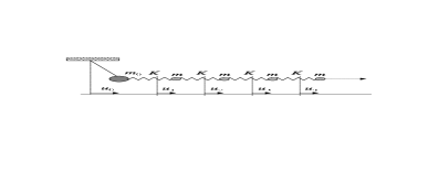
Figure 1: Scheme of the model: a simple pendulum (surface oscillator) is coupled to the bulk masses.

The equations of motion are,

$$\begin{array}[c]{l}\left[\dfrac{\mathrm{d}^{2}}{\mathrm{d}t^{2}}+\omega_{0}^{2}+\alpha\omega_{x}^{2}\right]u_{0}(t)-\alpha\omega_{x}^{2}u_{1}(t)=0,\\ \left[\dfrac{\mathrm{d}^{2}}{\mathrm{d}t^{2}}-2\omega_{x}^{2}\right]u_{n}(t)-\omega_{x}^{2}\left[u_{n-1}(t)+u_{n+1}(t)\right]=0,\end{array}$$ (1)

where $\omega_{x}=\sqrt{K/m}$ is the exchange frequency between neighbor oscillators and $u_{n}(t)$ denotes the $n$th oscillator displacement from equilibrium. Assuming that the number of bulk oscillators is finite, the time-reversal invariance present in these equations is obvious. We will show below how irreversibility appears in the thermodynamic limit where the number bulk oscillators become infinite.

II Frequency Domain

The equations of motion described above can be solved by Fourier transforming the displacement:

$$u_{n}(t)=\frac{1}{2\pi}\int_{-\infty}^{\infty}\mathrm{d}\omega e^{-\mathrm{i}\omega t}u_{n}(\omega),$$ (2)

and replacing it in Eq.(1):

$$\left(\omega^{2}\mathbb{I-M}\right)\mathbf{u}(\omega)=\mathbf{0}.$$ (3)

This equation is solved by the eigenfrequencies $\omega_{k}$ and eigenvectors $\mathbf{u}(\omega_{k})$ whose site components are expressed, in bracket notation, in terms of the site versors $\left\langle n\right|$ as

$$u_{n}(\omega_{k})=\left\langle n\left|\varphi_{k}\right.\right\rangle,$$ (4)

and the dynamical matrix is:

$$\mathbb{M=}\left(\begin{array}[c]{cccc}\omega_{0}^{2}+\alpha\omega_{x}^{2}&-\alpha\omega_{x}^{2}&0&\cdots\\ -\omega_{x}^{2}&2\omega_{x}^{2}&-\omega_{x}^{2}&\\ 0&-\omega_{x}^{2}&2\omega_{x}^{2}&\\ \vdots&&&\ddots\end{array}\right).$$ (5)

We define the Green’s function operator:

$$\mathbb{D}(\omega)=\left(\omega^{2}\mathbb{I-M}\right)^{-1},$$ (6)

whose matrix elements diverge when $\omega$ coincides with an eigenfrequency $\omega_{k}$.

Consider an initial condition with all masses at equilibrium and an impulsive force $m_{j}\dot{u}_{j}(0)\delta(t)$ applied to the $j$th mass, impossing an initial velocity to it. In this case, the Green’s function provides the time evolution of the $i$th mass displacement:

$$u_{i}(t)=D_{ij}(t)\dot{u}_{j}(0)=\frac{1}{2\pi}\int_{-\infty}^{\infty}\mathrm{d}\omega e^{-\mathrm{i}\omega t}D_{ij}(\omega)\dot{u}_{j}(0),$$ (7)

representing a position-velocity Green’s function $D_{ij}(\omega)\equiv D(u_{i},\dot{u}_{j};\omega)$, which is related to the position-position Green’s function:

$$D(u_{i},u_{j};\omega)=-\mathrm{i}\omega D(u_{i},\dot{u}_{j};\omega).$$ (8)

This gives the displacement of the $i$th mass when an initial displacement $u_{j}(0)$ is imposed by the force:

$$F_{j}(t)=m_{j}\frac{u_{j}(0)}{\tau}[\delta(t+\tfrac{1}{2}\tau)-\delta(t-\tfrac{1}{2}\tau)]$$ (9)

at the $j$th mass, where $\tau\ll 1/\omega_{x}$.

In this work, we focus on the surface oscillator through $D_{00}(t)$. If $\mathbb{U}$ is the matrix that performs the change of basis from sites to diagonal form in $\mathbb{M}$, one has:

$$U_{ik}=\left\langle i\right|\left.\varphi_{k}\right\rangle,$$ (10)

that is, the $k$th eigenmode projection over $i$th site. In this case one can write,

$$D_{00}(\omega)=\sum_{k}\frac{\left|\left\langle 0\right|\left.\varphi_{k}\right\rangle\right|^{2}}{\omega^{2}-\omega_{k}^{2}}.$$ (11)

By performing the analytical continuation $\omega\rightarrow\omega+\mathrm{i}\delta$ for $D_{00}(\omega)$ and taking its imaginary component, one obtains the spectral density associated to the surface site. In the case where $\alpha\rightarrow 0$ bulk modes and surface modes have no projection and oscillations survive undamped.

$D_{00}(\omega)$ can be obtained through an infinite order perturbation theory PM01 that accounts for the surface mode corrections due to the presence of the neighbor oscillators. Let us begin with the surface oscillator and a single bulk mass. If the two masses are uncoupled ($\omega_{x}=0$) the surface frequency is simply $\omega_{0}$ but if $\omega_{x}\neq 0$, Eq.(6) yields

$$D_{00}(\omega)=\frac{1}{\omega^{2}-\omega_{0}^{2}-\alpha\omega_{x}^{2}-\alpha\dfrac{\omega_{x}^{4}}{\omega^{2}-\omega_{x}^{2}}}.$$ (12)

Here, $\omega_{0}$ is affected by the static correction $\alpha\omega_{x}^{2}$ and the dynamic correction $\alpha\Pi(\omega)$ due to presence of the other oscillator.

By taking the limit of the oscillators number to infinite, the dynamic correction becomes

$$\Pi(\omega)=\frac{\omega_{x}^{4}}{\omega^{2}-2\omega_{x}^{2}-\Pi(\omega)}.$$ (13)

Because of the presence of an infinite number of oscillators at the right, a correction on the $n$th oscillator is just the same as that in the $(n+1)$th oscillator. The solution of Eq.(13) is complex and its imaginary part gives the decay rate of a surface excitation with frequency $\omega$. Therefore, in the thermodynamic limit, the temporal recurrences Blaise (Mesoscopic Echoes Mesoscopic ) disappear.

III Surface mode frequency

In the case of a surface oscillator with natural frequency $\omega_{0}$, coupled to an infinite number of bulk oscillators, the Green’s function is:

$$D_{00}(\omega)=\frac{1}{\omega^{2}-\omega_{0}^{2}-\alpha\omega_{x}^{2}-\alpha\Pi(\omega)}.$$ (14)

Hence, in the region of continuous modes ($\left|\omega\right|\leq 2\omega_{x}$) one has

$$D_{00}(\omega)=\frac{1}{1-\frac{\alpha}{2}}\frac{1}{\omega^{2}-\bar{\omega}_{0}^{2}+\mathrm{i}\eta(\omega)\omega},$$ (15)

where $\bar{\omega}_{0}=\omega_{0}/\sqrt{1-\alpha/2}$ is a first approximation to the resonance frequency and

$$\eta(\omega)=\frac{\alpha\omega_{x}}{1-\frac{\alpha}{2}}\sqrt{1-\left(\frac{\omega}{2\omega_{x}}\right)^{2}}$$ (16)

describes the dissipation process. Comparing Eq.(15) with a standard damped oscillator (frictional force proportional to velocity), it is easy to see that in the broadband limit ($\alpha\rightarrow 0,$ $\omega_{x}\rightarrow\infty$ and $\alpha\omega_{x}=\mathrm{const}$.) they have the same behavior taking $\eta_{0}\equiv\alpha\omega_{x}$ as friction coefficient.

For a dynamic description of the surface oscillator, we look for the pole structure of $D_{00}(\omega)$, equivalent to find $\omega$ such that:

$$\omega^{2}-\bar{\omega}_{0}^{2}+\mathrm{i}\eta(\omega)\omega=0.$$ (17)

If we denote the surface mode frequency as $\tilde{\omega}_{R}=\omega_{R}+\mathrm{i}\gamma_{R}$ and $p$ as

$$p=\frac{\omega_{0}-\omega_{x}}{\omega_{x}\sqrt{1-\alpha}},$$ (18)

then one has

$$\tilde{\omega}_{R}=\left\{\begin{array}[c]{cc}-\sqrt{\omega_{0}^{2}+\delta\left[\omega_{-}^{2}+\sqrt{\omega_{+}^{4}-4\omega_{x}^{2}\omega_{0}^{2}}\right]}&p<-1\\ \sqrt{\omega_{0}^{2}+\delta\left[\omega_{-}^{2}-\mathrm{i}\sqrt{4\omega_{x}^{2}\omega_{0}^{2}-\omega_{+}^{4}}\right]}&\left|p\right|\leq 1\\ \sqrt{\omega_{0}^{2}+\delta\left[\omega_{-}^{2}-\sqrt{\omega_{+}^{4}-4\omega_{x}^{2}\omega_{0}^{2}}\right]}&p>1\end{array}\right.$$

where $\omega_{\mathrm{\pm}}^{2}=\omega_{0}^{2}\pm\alpha\omega_{x}^{2}$ and $\delta=\alpha/2(1-\alpha)$. The dependence of the pole with $\omega_{0}$ can be seen in Fig.2.

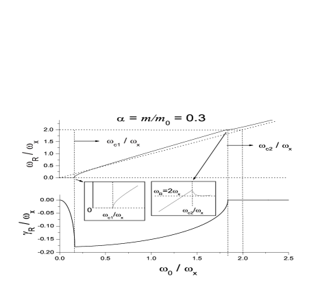
Figure 2: Surface Green’s function pole. Above: real part (resonance). Below: imaginary part (damping). The case $\omega_{R}=\omega_{0}$ is shown in dotted line. Insets: overdamped - oscillatory transition (left), oscillatory - localized (right).

Here, we show the real and imaginary parts of the pole separately and we find three well-defined regimes that emphasize the onset of quite different dynamical properties.

IV Dynamical phases

Localized - extended transition. This transition occurs when $\omega_{0}$ lays close to the upper band edge. There, the real part of the pole makes an excursion into the band gap conserving an imaginary component which is lost at the cusp zoomed in the inset. This is analogous to the virtual states described by Hogreve Hogreve for electronic states which are missed under other approximations Economou ; Desjonqueres . They become real normalized states which are exponentially localized Taylor when the pole touches back the band edge.

It can be seen in Fig.2 that for large values of surface natural frequency $(\omega_{0}\gg 2\omega_{x})$ we only have real component in $\tilde{\omega}_{R}$ and the oscillation frequency is approximately $\omega_{0}$. In this localized regime, displacements are exponentially smaller as the oscillators increase their distance to the surface. The lack of an imaginary part implies that the displacement amplitude, independently of bulk oscillators, survives indefinitely. In other words, there is no energy propagation to bulk oscillators.

As $\omega_{0}$ decreases, below a critical frequency $\omega_{c2}=\omega_{x}(1+\sqrt{1-\alpha})$, $\tilde{\omega}_{R}$ becomes complex. Its real part is the resonance frequency whereas its imaginary part describes the dissipation. This is the extended oscillatory regime where surface oscillations have an $\omega_{R}$ frequency and the amplitude of displacement decays with a lifetime proportional to $1/\gamma_{R}$.

Oscillatory - overdamped transition. For $\omega_{0}\ll\omega_{x}$ the system is in the regime where $\eta(\omega)\simeq\alpha\omega_{x}/(1-\alpha/2)$ and hence Eq.(17) yields Ohmic dissipation in which the surface kinetic energy decays into bulk modes without return. This describes a frictional force proportional to the velocity. As $\omega_{0}$ goes below the critical frequency $\omega_{c1}=\omega_{x}(1-\sqrt{1-\alpha})$, the pole of the Green’s function $\tilde{\omega}_{R}$ becomes purely imaginary. This is the overdamped regime where no oscillations occur. Notice that $\gamma_{R}$ decreases at both sides of the transition, this means that a further decrease of $\omega_{0}$ or increase in the friction $\eta$ also implies a decrease in the relaxation rate. All this counter intuitive effect arrises from the exact solution of the simple mechanical model.

Considering Eq.(7), we can complete our previous analysis obtaining the time evolution of surface displacement by performing a numerical Fourier transform of the analytical expression for $D_{00}(\omega)$. These results coincide with the numerical integration of the equation of motion in the Hamilton-Jacobi representation which is performed with an ad hoc version of the Trotter-Suzuki method Trotter-Suzuki . Setting the ratio $\alpha$ between masses and Fourier transforming for several $\omega_{0}$ values in the previously mentioned regimes, we obtain the displacement pattern shown in Fig.3.

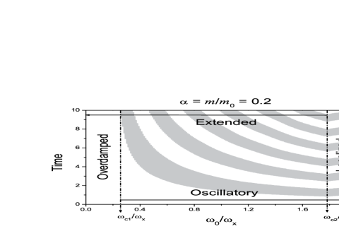
Figure 3: Evolution of the surface displacement. White spaces denote $u_{0}(t)>0$ whereas gray spaces denote $u_{0}(t)<0$.

Here, the time evolution of the surface displacement depends on the initial condition. It is easy to see in this picture how gray regions ”diverge” near the critical frequency $\omega_{c1}$ so that for smaller $\omega_{0}$ values $u_{0}(t)$ is always positive. On the other hand, the period of the oscillation (reflected from the fringe edges) shows a cusp at $\omega_{c2}$ where it start to increase again. This is consistent with the decrease of $\omega_{R}$ as $\omega_{0}$ crosses $\omega_{c2}$ (see inset in Fig.2).

V Conclusions

Dynamical features in dissipation processes have been described by a simple classical model that contains the essential properties of a surface oscillator interacting with bulk vibrational modes. We arrive to results equivalent to the phenomenological description of dissipation where these effects are summarized in a single term proportional to the oscillator velocity. A complete analytical solution of the dynamics allowed us to identify a variety of dynamical phases available for the vibrational excitations: localized, extended oscillatory and overdamped. Two numerical methods (FFT and a Trotter-Suzuki algorithm) have been employed to obtain the dynamics with equivalent results.

The identification of the different dynamical regimes becomes very important in nano-physics when cantilevers Cantilever involving a relative small number of atoms fail to satisfy the standard thermodynamical approximations. Localization, weak diffusion and recurrences become usual phenomena in the nanomechanical devices. In a quantum description of finite size systems, we should consider the quantization of oscillation amplitudes. Our formalism, based on the Green’s functions in discrete but open systems, seems to be the ideal tool for this purpose.

References

- (1) R. Feynman, The Feynman Lectures on physics, vol. I, Ch. 23-25, Addison-Wesley, 1970.
- (2) T. Dittrich, P. Hänggi, G.-L. Ingold, B. Kramer, G. Schön, W. Zwerger, Quantum transport and dissipation, 217, Wiley-VCH, 1998.
- (3) R. J. Rubin, Phys. Rev. 131 3, 964 (1963).
- (4) P. Hänggi and G.-L. Ingold, Chaos 15,026105 (2005)
- (5) H. M. Pastawski and E. Medina, Rev. Mex. Física 47s1, 1 (2001), cond-mat/0103219.
- (6) P. Blaise, P. Durand and O. Henri-Rousseau, Phys. A 209, 51 (1994).
- (7) H.M. Pastawski, P. R. Levstein and G. Usaj, Phys. Rev. Lett. 75, 4310 (1995).
- (8) H. Hogreve, Phys. Lett. A 201, 111 (1995).
- (9) E. N. Economou, Green’s functions in quantum physics, Springer series in solid state physics 7, 1979.
- (10) M.C. Desjonquères and D. Spanjaard, Concepts in Surface Physics 2, 114, Springer, 1996.
- (11) P. L. Taylor, A quantum approach to the Solid State, Prentice-Hall, 290, 1967.
- (12) H. De Raedt, Ann. Rev. of Comp. Physics IV, 107 (1996).
- (13) K. C. Schwab and M. L. Roukes, Physics Today 58, 36 (2005).