Full counting statistics of spin transfer through the Kondo dot

Abstract

We calculate the spin current distribution function for a Kondo dot in two different regimes. In the exactly solvable Toulouse limit the linear response, zero temperature statistics of the spin transfer is trinomial, such that all the odd moments vanish and the even moments follow a binomial distribution. On the contrary, the corresponding spin-resolved distribution turns out to be binomial. The combined spin and charge statistics is also determined. In particular, we find that in the case of a finite magnetic field or an asymmetric junction the spin and charge measurements become statistically dependent. Furthermore, we analyzed the spin counting statistics of a generic Kondo dot at and around the strong-coupling fixed point (the unitary limit). Comparing these results with the Toulouse limit calculation we determine which features of the latter are generic and which ones are artifacts of the spin symmetry breaking.

I Introduction

It has been known for some time that the current noise spectra of mesoscopic systems can reveal information about transport processes which is not accessible via measurement of the average current alone. Indeed, it has been shown by Schottky Schottky (1918) that the characteristics of charge carriers can be investigated by measuring noise spectra. The noise is the second moment of the distribution function which gives the probability that a certain amount of charge is transported within a certain time interval $\mathcal{T}$. Recent developments in experimental mesoscopic physics have facilitated the measurement of even higher order moments of this distribution.Reulet et al. (2003) Therefore, it is desirable to calculate the complete statistics, which is often referred to as the full counting statistics (FCS). The FCS has been found for the charge transport in non-interacting systems by Levitov and Lesovik Levitov and Lesovik (1993) and, currently, interaction effects are under intensive investigation.

Recent years have witnessed a soaring interest in the field of spintronics,Awschalom et al. (2002) where the principal objective is to gain a level of control over spin transport (which comprises creation of current and its measurement) comparable to that over charge transport. Indeed, the usage of the electron spin degree of freedom offers many enticing opportunities which are currently being investigated. Therefore, in order to gain a thorough understanding of spin-related processes taking place in mesoscopic systems, one has to understand the properties of spin current to the same level of accuracy as the charge current.

A method of measuring spin currents and some intriguing consequences of consecutive measurements of different spin components have been presented by Di Lorenzo and Nazarov.Lorenzo and Nazarov (2004) Although some general statements about spin transfer FCS have been made there, to the best of our knowledge, there has so far been no derivation of the spin transfer FCS for a concrete system. The aim of this article is to fill this gap. While the charge FCS was shown to be binomial, at least in the universal linear response, zero temperature limit,Gogolin and Komnik (2006a) it is not immediately clear what the nature of the spin statistics should be: the natural guess that it is the inverse binomial distributionMandel and Wolf (1995) (due to bosonic nature of spin excitations) turns out to be wrong. The purpose of this article is to investigate the spin transfer FCS for the transport through a Kondo dot, where non-zero spin currents can be relatively easily generated by applying a finite magnetic field and a bias voltage. Furthermore, we go one step further and calculate the combined FCS of charge and spin transfer, which will allow us to examine cross-correlations of these two currents and to obtain spin-resolved charge transfer statistics.

We shall perform this analysis on two distinct systems which represent two aspects of the Kondo physics. First, we will investigate a Kondo dot at the Toulouse point, where for a certain choice of coupling constants, the system can be diagonalized exactly by means of bosonization and subsequent refermionization. Second, we will go to the strong-coupling regime where the dot spin is hybridized with the leads spins to form a singlet state. Virtual excitations of this singlet state can be treated perturbatively and will be shown to produce a finite spin current noise. This article will close with a comparison of these two regimes.

II Hamiltonian

The system under investigation consists of two non-interacting leads and an interacting dot level. The left/right leads are being held at chemical potentials $\mu_{L/R}$, respectively, where $V=(\mu_{L}-\mu_{R})/e$ is the applied voltage. The position of the bare dot level and the electron-electron repulsion are such that the dot is always occupied by exactly one electron. The result is the two-channel Kondo Hamiltonian,Schiller and Hershfield (1998) $H=H_{0}+H_{K}+H_{B}+Y_{0}$, where (in units of $e=\hbar=v_{F}=1$),

$$H_{0} = i\sum_{\alpha=LR}\sum_{\sigma=\uparrow\downarrow}\int dx\psi_{\alpha\sigma}^{\dagger}(x)\partial_{x}\psi_{\alpha\sigma}(x)\,,$$

$$H_{K} = \sum_{\alpha\beta=LR}\sum_{\nu=x,y,z}J^{\alpha\beta}_{\nu}s^{\nu}_{\alpha\beta}\tau^{\nu}\,,$$

$$H_{B} = -\mu_{B}gh\tau^{z}=:-\Delta\tau^{z}\,,$$

$$Y_{0} = \frac{V}{2}\sum_{\sigma=\uparrow\downarrow}\int dx\left[\psi_{L\sigma}^{\dagger}\psi_{L\sigma}-\psi_{R\sigma}^{\dagger}\psi_{R\sigma}\right]\,.$$ (1)

In this equation, $\tau^{x,y,z}$ are proportional to the Pauli matrices describing the impurity spin, $J^{\alpha\beta}_{\nu}$ for $\alpha,\beta=L,R$ and $\nu=x,y,z$ are coupling constants for the possible transport processes, $h$ is the magnetic field applied to the dot level. Furthermore,

$$\vec{s}_{\alpha\beta}=\frac{1}{2}\sum_{\sigma,\sigma^{\prime}}\psi_{\alpha\sigma}^{\dagger}(0)\vec{\tau}_{\sigma\sigma^{\prime}}\psi_{\beta\sigma^{\prime}}(0)\,,$$ (2)

for $\alpha,\beta=L,R$ are the components of the electron spin density at the impurity site.

The aim of FCS is the calculation of the cumulant generating function (CGF) $\chi(\mu,\lambda)$ for the probability distribution function $P(s,q)$ to transfer $q$ units of charge and $s$ units of spin during the waiting time $\mathcal{T}$. In our case, as we are interested in the combined statistics of spin transfer and charge transfer, we define $\chi(\mu,\lambda)=\sum_{s,q}e^{is\mu}e^{iq\lambda}P(s,q)$. Partial derivatives of this function then allow us to calculate arbitrary correlation functions of charge and spin transport and cross-correlations between both.

In order to calculate spin and charge current in this system, we proceed as usually in tunneling setups and define charge and spin flavor number operators

$$N_{c} = \frac{1}{2}\sum_{\alpha=LR}\sum_{\sigma=\uparrow\downarrow}\alpha\int dx\psi^{\dagger}_{\alpha\sigma}(x)\psi_{\alpha\sigma}(x)\,,$$ (3)

$$N_{s} = \frac{1}{2}\sum_{\alpha=LR}\sum_{\sigma=\uparrow\downarrow}\alpha\sigma\int dx\psi^{\dagger}_{\alpha\sigma}(x)\psi_{\alpha\sigma}(x)\,.$$ (4)

The time derivatives of these operators are proportional to the charge and spin currents, respectively. Hence, the corresponding charge and spin currents can be calculated by means of the Heisenberg equation $I_{c,s}=i[H,N_{c,s}]$. The general approach to calculate higher order cumulants of these operators involves including fictitious measurement devices for both charge and spin current in the Hamiltonian.Nazarov and Kindermann (2003) This leads to additional terms $H_{m}=\mu I_{s}+\lambda I_{c}$. As in our case the particle number operators $N_{c}$ and $N_{s}$ commute, both terms can be removed by a unitary transformation. The counting fields $\mu$ and $\lambda$ then appear as exponentials in those components of the Hamiltonian which transfer spin or charge in either direction:Levitov and Reznikov (2004) from the left lead to the right, $T^{c,s}_{L}$, and backwards, $T^{c,s}_{R}$. As in this case the underlying processes for spin and charge transport will be different, the tunneling Hamiltonian separates into spin and charge parts and becomes [see Eq. (10)]

$$T^{\mu\lambda} = e^{i\mu(t)}T^{s}_{L}+e^{-i\mu(t)}T^{s}_{R}$$ (5)

$$+ e^{i\lambda(t)}T^{c}_{L}+e^{-i\lambda(t)}T^{c}_{R}\,,$$

where $\mu(t)$ and $\lambda(t)$ are explicitly time-dependent functions defined on the Keldysh contour $C$. The counting fields are only “switched on” during the measurement time $\mathcal{T}$​, such that we can define them as $\mu(t_{\pm})=\pm\mu\theta(t)\theta(\mathcal{T}-t)$ and analogously for $\lambda(t_{\pm})$. The CGF is then given by the expectation valueLevitov and Reznikov (2004)

$$\chi(\mu,\lambda)=\left\langle T_{C}\ e^{-i\int_{C}dsT^{\mu\lambda}(s)}\right\rangle,$$ (6)

where $T_{C}$ denotes the contour ordering operator. In order to calculate this function, we employ the generalized Green’s function formalism that has previously been used successfully to calculate the FCS of other interacting systems: Komnik and Gogolin (2005); Gogolin and Komnik (2006a) We assume $\lambda(s)$ and $\mu(s)$ to be arbitrary functions defined on $C$ that have slowly varying Keldysh components $\lambda_{\pm}(t)$ and $\mu_{\pm}(t)$, respectively. Assuming $\mathcal{T}$ to be large, we can neglect processes which are due to the switching of the counting fields, and we can introduce the adiabatic potential $U(\mu_{\pm},\lambda_{\pm})$ which entails

$$\chi[\mu_{\pm}(t),\lambda_{\pm}(t)]=e^{-i\int_{0}^{\mathcal{T}}dtU[\mu_{\pm}(t),\lambda_{\pm}(t)]}\,,$$ (7)

from which the statistics can be recovered using the equation $\ln\chi(\mu,\lambda)=-i\mathcal{T}U(\mu,\lambda)$ as $U(\mu,\lambda)$ will turn out to be time-independent. By comparison of (6) and (7), one notices that the adiabatic potential can be calculated due to the following relation (which is a consequence of the Feynman-Hellmann theorem)

$$\frac{\partial U}{\partial\lambda_{-}}=\left\langle\frac{\partial T^{\mu\lambda}}{\partial\lambda_{-}}\right\rangle_{\mu\lambda}$$ (8)

or, equivalently, via the partial derivative with respect to $\mu_{-}$. The expectation value with subscript $\mu\lambda$ is defined as expectation value in the interaction picture with respect to the tunneling Hamiltonian $T^{\mu\lambda}$, ie.Komnik and Gogolin (2005); Gogolin and Komnik (2006a)

$$\left\langle A(t)\right\rangle_{\mu\lambda}=\frac{1}{\chi(\mu_{\pm},\lambda_{\pm})}\left\langle T_{C}\left\{A(t)e^{-i\int_{C}dsT^{\mu\lambda}(s)}\right\}\right\rangle.$$ (9)

The emerging expression is slightly more complicated than the usual Hamiltonian formalism. However, the great advantage of using the derivatives of $U$ is the emergence of Green’s functions (the time dependence of which is dominated by $T^{\mu\lambda}$) for which a Dyson equation can be obtained. Then, the adiabatic potential $U(\mu,\lambda)$ can be recovered by integrating (8) (or, equivalently, the derivative with respect to $\mu_{-}$, the result is the same) which, in turn, leads immediately to the CGF $\chi(\mu,\lambda)$.

III Dyson equation at the Toulouse point

For a general constellation of system parameters, $\chi(\mu,\lambda)$ cannot be calculated exactly. The perturbation theory in the exchange couplings is well known to diverge logarithmically and so is not very useful in calculating the FCS. However, it has been realized by Toulouse that the Kondo Hamiltonian can be reduced to an easily integrable shape for a special parameter set. Toulouse (1969) In our notation this so-called Toulouse point is attained for $J^{\alpha\beta}_{x}=J^{\alpha\beta}_{y}=:J^{\alpha\beta}_{\perp},J^{LR}_{\perp}=J^{RL}_{\perp}$ and $J^{LR}_{z}=J^{RL}_{z}=0$.Schiller and Hershfield (1998) The only allowed processes are then: (i) spin-flip tunneling which transports one unit of charge but does not contribute to the spin current, and (ii) spin-exchange between one lead and the dot which only transports one unit of spin with no associated charge transport. Furnishing both processes with the respective counting fields $\mu(t)$ and $\lambda(t)$ the tunneling operator becomes

$$T^{\mu\lambda} = \frac{J^{LL}_{\perp}}{2}\Big{[}\psi_{L\uparrow}^{\dagger}\psi_{L\downarrow}e^{-i\mu/2}\tau^{-}+\psi_{L\downarrow}^{\dagger}\psi_{L\uparrow}e^{i\mu/2}\tau^{+}\Big{]}$$ (10)

$$+ \frac{J^{RR}_{\perp}}{2}\Big{[}\psi_{R\uparrow}^{\dagger}\psi_{R\downarrow}e^{i\mu/2}\tau^{-}+\psi_{R\downarrow}^{\dagger}\psi_{R\uparrow}e^{-i\mu/2}\tau^{+}\Big{]}$$

$$+ \frac{J^{LR}_{\perp}}{2}\Big{[}\psi_{L\uparrow}^{\dagger}\psi_{R\downarrow}e^{-i\lambda/2}\tau^{-}+\psi_{L\downarrow}^{\dagger}\psi_{R\uparrow}e^{-i\lambda/2}\tau^{+}$$

$$+ \psi_{R\uparrow}^{\dagger}\psi_{L\downarrow}e^{i\lambda/2}\tau^{-}+\psi_{R\downarrow}^{\dagger}\psi_{L\uparrow}e^{i\lambda/2}\tau^{+}\Big{]}.$$

In the next step, we proceed along the lines of Schiller and Hershfield:Schiller and Hershfield (1998) First, we bosonize the Hamiltonian by introducing four bosonic fields describing total charge (c), charge flavor (f), total spin (s) and spin flavor (sf). Then, we perform an Emery-KivelsonEmery and Kivelson (1992) rotation and refermionize the Hamiltonian. After going to the Toulouse point $J^{LL}_{z}=J^{RR}_{z}=:J_{z}:=2\pi$, the total spin field decouples and the resulting Hamiltonian is quadratic in the three remaining fermionic fields. The unperturbed part reads

$$H_{0} = i\sum_{\nu}\int dx\psi^{\dagger}_{\nu}(x)\partial_{x}\psi_{\nu}(x)\,,$$

$$H_{B} = \Delta(d^{\dagger}d-1/2)\,,$$

$$Y_{0} = V\int dx\psi^{\dagger}_{f}(x)\psi_{f}(x)\,,$$ (11)

where $d=i\tau^{+}$ is the fermion operator describing the dot spin and $\nu\in\{c,f,sf\}$. The tunneling part becomes

$$T^{\mu\lambda} = -\frac{J^{LL}_{\perp}}{2\sqrt{2\pi a_{0}}}\left[e^{-i\mu/2}d^{\dagger}\psi^{\dagger}_{sf}-e^{i\mu/2}d\psi_{sf}\right]$$ (12)

$$- \frac{J^{RR}_{\perp}}{2\sqrt{2\pi a_{0}}}\left[e^{i\mu/2}d^{\dagger}\psi_{sf}-e^{-i\mu/2}d\psi^{\dagger}_{sf}\right]$$

$$- \frac{J^{LR}_{\perp}}{2\sqrt{2\pi a_{0}}}\Big{[}e^{-i\lambda/2}d^{\dagger}\psi^{\dagger}_{f}+e^{-i\lambda/2}d\psi^{\dagger}_{f}$$

$$- e^{i\lambda/2}d^{\dagger}\psi_{f}-e^{i\lambda/2}d\psi_{f}\Big{]}\,,$$

where $a_{0}$ is the lattice constant of the underlying lattice model which emerges in the bosonization process. Note that $T^{\mu\lambda}$ only contains $\psi_{f}$ and $\psi_{sf}$ which means that $\psi_{c}$ is completely decoupled and can safely be discarded. Physically, this is due to the fact that the total charge in conserved in the system. Next, we split the relevant fields into hermitian components (Majorana fermions) according to $\psi_{sf}=(\xi+i\eta)/\sqrt{2}$, $\psi_{f}=(\zeta+i\epsilon)/\sqrt{2}$, $d=(a+ib)/\sqrt{2}$, and obtain the Hamiltonian

$$H=H_{0}+iV\int dx\,\zeta(x)\epsilon(x)-i\Delta ab+T^{\mu\lambda}\,,$$ (13)

where the tunneling operator is given by

$$T^{\mu\lambda} = iJ_{-}\sin(\mu/2)a\xi+iJ_{+}\cos(\mu/2)b\xi$$ (14)

$$+ iJ_{-}\cos(\mu/2)a\eta-iJ_{+}\sin(\mu/2)b\eta$$

$$+ iJ_{\perp}\sin(\lambda/2)a\zeta+iJ_{\perp}\cos(\lambda/2)a\epsilon\,.$$

In this equation, we have introduced $J_{\pm}=(J^{LL}_{\perp}\pm J^{RR}_{\perp})/(2\sqrt{2\pi a_{0}})$ and $J_{\perp}=J^{LR}_{\perp}/(\sqrt{2\pi a_{0}})$. According to (8), the next step is to calculate the expectation value of the partial derivatives of $T^{\mu\lambda}$ which can easily be calculated from (14). If we calculate the derivative with respect to, say, $\lambda_{-}$,

$$\left\langle\frac{\partial T^{\mu\lambda}}{\partial\lambda_{-}}\right\rangle_{\mu\lambda}=-\frac{J_{\perp}}{2}\big{[}\cos(\lambda_{-}/2)G^{--}_{a\zeta}-\sin(\lambda_{-}/2)G^{--}_{a\epsilon}\big{]}\,,$$ (15)

we obtain an expression which contains the Green’s functions

$$G^{--}_{a\zeta}(t,t^{\prime}) = -i\left\langle Ta(t)\zeta(t^{\prime})\right\rangle_{\mu\lambda}$$ (16)

$$G^{--}_{a\epsilon}(t,t^{\prime}) = -i\left\langle Ta(t)\epsilon(t^{\prime})\right\rangle_{\mu\lambda}$$ (17)

where the time arguments $t,t^{\prime}$ are located on the “$-$”-branch of the Keldysh contour and, consequently, are time-ordered. Expanding (16) to first order in $J_{\perp}$, one can express it in terms of the exact dot Green’s function $D_{aa}(t,t^{\prime})=-i\left\langle T_{C}a(t)a(t^{\prime})\right\rangle_{\mu\lambda}$. Assuming the counting fields $\mu_{\pm}(t)$ and $\lambda_{\pm}(t)$ to be time-independent on the respective branches of the Keldysh contour, we have

$$G^{--}_{a\zeta}(\omega) = iJ_{\perp}\Big{[}s_{-}D^{--}_{aa}G^{(0)--}_{\zeta\zeta}+c_{-}D^{--}_{aa}G^{(0)--}_{\epsilon\zeta}$$ (18)

$$- s_{+}D^{-+}_{aa}G^{(0)+-}_{\zeta\zeta}-c_{+}D^{-+}_{aa}G^{(0)+-}_{\epsilon\zeta}\Big{]}\,,$$

where $s_{\pm}=\sin(\lambda_{\pm}/2)$ and $c_{\pm}=\cos(\lambda_{\pm}/2)$. An analogous equation can be derived for $G_{a\epsilon}$. The exact dot Green’s function can be derived by means of a Dyson equation which in Fourier space reads $\mathbb{D}=\mathbb{D}^{(0)}+\mathbb{D}\bf{\Sigma}\mathbb{D}^{(0)}$. The matrix of dot Green’s function is defined by

$$\mathbb{D}=\left(\begin{array}[]{cccc}D^{--}_{aa}&D^{-+}_{aa}&D^{--}_{ab}&D^{-+}_{ab}\\ D^{+-}_{aa}&D^{++}_{aa}&D^{+-}_{ab}&D^{++}_{ab}\\ D^{--}_{ba}&D^{-+}_{ba}&D^{--}_{bb}&D^{-+}_{bb}\\ D^{+-}_{ba}&D^{++}_{ba}&D^{+-}_{bb}&D^{++}_{bb}\\ \end{array}\right)$$ (19)

and the self-energy $\bf{\Sigma}$ is defined as a block matrix coupling the Majorana components $a$ and $b$ of the dot operator,

$$\bf{\Sigma}=\left(\begin{array}[]{cc}M_{aa}&M_{ab}\\ M_{ba}&M_{bb}\\ \end{array}\right)\,.$$ (20)

It turns out that this matrix only depends on $\lambda:=(\lambda_{-}-\lambda_{+})/2$ and $\mu:=(\mu_{-}-\mu_{+})/2$. We therefore introduce the shorthand notation $s_{\mu,\lambda}=\sin(\mu,\lambda)$ and $c_{\mu,\lambda}=\cos(\mu,\lambda)$. The non-diagonal elements are then given by

$$M_{ab}=J_{-}J_{+}\left(\begin{array}[]{cc}0&-s_{\mu}G^{(0)-+}_{\xi\xi}\\ s_{\mu}G^{(0)+-}_{\xi\xi}&0\\ \end{array}\right)$$ (21)

and $M_{ba}=-M_{ab}$. Next, we have for the $M_{bb}$ element

$$M_{bb}=J_{+}^{2}\left(\begin{array}[]{cc}G^{(0)--}_{\xi\xi}&-c_{\mu}G^{(0)-+}_{\xi\xi}\\ -c_{\mu}G^{(0)+-}_{\xi\xi}&G^{(0)++}_{\xi\xi}\\ \end{array}\right)\,.$$ (22)

These three matrices do not involve the charge counting field $\lambda$ which is a consequence of the fact that the $\lambda$-dependent part of the tunneling operator (14) only couples to the Majorana fields $a$. The only $\lambda$-dependent contribution in the Dyson equation arises from the $M_{aa}$ component which is given by

$$M_{aa} = J_{-}^{2}\left(\begin{array}[]{cc}G^{(0)--}_{\xi\xi}&-c_{\mu}G^{(0)-+}_{\xi\xi}\\ -c_{\mu}G^{(0)+-}_{\xi\xi}&G^{(0)++}_{\xi\xi}\\ \end{array}\right)+J^{2}_{\perp}\left(\begin{array}[]{cc}G^{(0)--}_{\zeta\zeta}&-c_{\lambda}G^{(0)-+}_{\zeta\zeta}+s_{\lambda}G^{(0)-+}_{\epsilon\zeta}\\ -c_{\lambda}G^{(0)+-}_{\zeta\zeta}-s_{\lambda}G^{(0)+-}_{\epsilon\zeta}&G^{(0)++}_{\zeta\zeta}\\ \end{array}\right)\,.$$ (27)

As the zero order lead and dot Green’s functions are well known,Komnik and Gogolin (2005) solving the Dyson equation amounts to inverting a $4\times 4$-matrix. The ensuing calculation is lengthy but straightforward. The result is an expression for the exact dot Green’s function, which can be used to evaluate (15). The equation can then be integrated to obtain the adiabatic potential $U(\mu,\lambda)$ which in turn determines the CGF.

IV Cumulant generating function

Finally, one obtains the CGF which describes the combined statistics of charge and spin transport and which is the main result of this article,

$$\ln\chi(\mu,\lambda) = \mathcal{T}\int_{0}^{\infty}\frac{d\omega}{2\pi}\ln\bigg{\{}1+\frac{1}{D(\omega)}\Big{\{}\kappa(e^{i2\mu}+e^{-i2\mu}-2)$$ (28)

$$+ \sum\limits_{p=\pm}\Big{[}\alpha_{p}(e^{i2p\lambda}-1)+\nu_{p}(e^{i\mu}-e^{-i\mu})e^{ip\lambda}$$

$$+ \beta_{p}\left(e^{i(\mu+p\lambda)}+e^{-i(\mu-p\lambda)}-2\right)$$

$$+ \rho_{p}\left(e^{i2(\mu+p\lambda)}+e^{-i2(\mu-p\lambda)}-2\right)\Big{]}\Big{\}}\bigg{\}}\,,$$

where $\Gamma_{i}=J_{i}^{2}/2$ and

$$D(\omega) = \left[\omega^{2}-\Delta^{2}-\Gamma_{+}(\Gamma_{\perp}+\Gamma_{-})\right]^{2}$$ (29)

$$+ \omega^{2}\left(\Gamma_{+}+\Gamma_{-}+\Gamma_{\perp}\right)^{2}.$$

Defining $n_{F}(\omega),n_{R}(\omega)$ and $n_{L}(\omega)$ to be the Fermi functions with chemical potentials $0$, $-V/2$ and $V/2$, respectively, the ‘transmission coefficients’ are given by

$$\alpha_{+} = n_{L}(1-n_{R})\left[1+2n_{F}(n_{F}-1)\right]\Gamma_{+}^{2}\Gamma_{\perp}^{2}$$

$$+ \omega^{2}\,n_{L}(1-n_{R})\Gamma_{\perp}^{2}\,,$$

$$\beta_{+} = \left[n_{F}(1-n_{R})+n_{L}(1-n_{F})\right]\Gamma_{+}\Gamma_{\perp}(\Gamma_{-}\Gamma_{+}+\Delta^{2})$$

$$+ \omega^{2}\,\left[n_{F}(1-n_{R})+n_{L}(1-n_{F})\right]\Gamma_{-}\Gamma_{\perp}\,,$$

$$\kappa = \left[n_{R}(1-n_{L})+n_{L}(1-n_{R})-1\right]n_{F}(n_{F}-1)\Gamma_{+}^{2}\Gamma_{\perp}^{2}$$

$$+ \omega^{2}n_{F}(1-n_{F})\left(\Gamma_{-}-\Gamma_{+}\right)^{2}\,,$$

$$\rho_{+} = n_{L}(1-n_{R})n_{F}(1-n_{F})\Gamma_{+}^{2}\Gamma_{\perp}^{2}\,,$$

$$\nu_{+} = 2\omega\left[n_{F}(n_{L}-n_{R}+1)-n_{L}\right]\sqrt{\Gamma_{-}\Gamma_{+}}\Gamma_{\perp}\Delta\,,$$ (30)

where all the quantities with opposite subscripts are given by the same expressions with interchanged $R$ and $L$ indices. From (28), one can easily calculate all correlation functions of charge and spin currents. In particular, by setting $\mu=0$, one immediately recovers the known charge transfer statistics for this system.Komnik and Gogolin (2005) Before returning to the complete statistics (28), we shall investigate in more detail the spin transfer statistics. By setting $\lambda=0$, we obtain the CGF for the spin transfer,

$$\ln\chi(\mu) = \mathcal{T}\int_{0}^{\infty}\frac{d\omega}{2\pi}\ln\bigg{\{}1+T_{1a}(n_{F}-n)(e^{i\mu}-e^{-i\mu})$$ (31)

$$+ T_{1s}\left[n(1-n_{F})+n_{F}(1-n)\right](e^{i\mu}+e^{-i\mu}-2)$$

$$+ T_{2}n_{F}(1-n_{F})(e^{2i\mu}+e^{-2i\mu}-2)\bigg{\}}$$

where $n=(n_{L}+n_{R})/2$ and the ‘transmission coefficients’ are given by

$$T_{1a}(\omega) = \frac{4}{D(\omega)}\left[\sqrt{\Gamma_{-}\Gamma_{+}}\Gamma_{\perp}\Delta\omega\right],$$

$$T_{1s}(\omega) = \frac{2}{D(\omega)}\left[\Gamma_{+}\Gamma_{\perp}\left(\Gamma_{-}\Gamma_{+}+\Delta^{2}\right)+\Gamma_{-}\Gamma_{\perp}\omega^{2}\right],$$

$$T_{2}(\omega) = \frac{1}{D(\omega)}\left[\Gamma_{+}^{2}\Gamma_{\perp}^{2}+(\Gamma_{-}-\Gamma_{+})^{2}\omega^{2}\right].$$ (32)

One can see that two kinds of processes contribute to the statistics. The coefficients $T_{1s}$ and $T_{1a}$ represent symmetric and anti-symmetric tunneling events in which one unit of spin is transferred. Therefore, $T_{1a}$ controls the odd cumulants, in particular the average spin current whereas $T_{1s}$ only influences even cumulants like the noise. Odd cumulants obviously vanish for a symmetric system ($\Gamma_{-}=0$) or zero magnetic field ($\Delta=0$). On the other hand, $T_{2}$ involves voltage-independent processes which transfer two units of spin. Those are coupled spin-flip processes which do not involve electron tunneling and can only occur at finite temperatures, see Fig. 1.

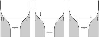
Figure 1: Schematic representation of the process $T_{2}$.

V Special regimes

V.1 Zero temperature case

Next, we shall address some special regimes and begin with the zero temperature case. In the limit of low energy we obtain the following statistics,

$$\chi(\mu)=\Big{[}(1-T_{1s})+\frac{1}{2}T_{1s}\left(e^{i\mu}+e^{-i\mu}\right)\Big{]}^{N}.$$ (33)

This is basically a symmetric trinomial distribution. Restoring SI units, the exponent can be written as $N=eV\mathcal{T}/h$, in which case $N$ can be interpreted as the number of ‘attempts’,Levitov et al. (1996) i.e. the number of electrons impinging on the tunneling contact in time $\mathcal{T}$. Comparing it with the corresponding distribution function for the charge transfer,Komnik and Gogolin (2005) one concludes that (33) is the same distribution with odd moments removed. Hence, the lowest order average spin current is quadratic in $V$, precisely as found by Schiller and Hershfield.Schiller and Hershfield (1998) The noise in the zero temperature limit, however, is linear in $V$,

$$\langle\!\langle\delta s^{2}\rangle\!\rangle = \frac{\mathcal{T}V}{\pi}\frac{\Gamma_{+}\Gamma_{\perp}\left(\Gamma_{-}\Gamma_{+}+\Delta^{2}\right)}{\left[\Delta^{2}+\Gamma_{+}(\Gamma_{\perp}+\Gamma_{-})\right]^{2}}$$ (34)

$$= \frac{\mathcal{T}V}{\pi}T_{0}\left[1-T_{0}\right]\,,$$

where $\delta s=\int_{0}^{\mathcal{T}}dtI_{s}(t)$ in the spin transferred during the measurement time $\mathcal{T}$. $T_{0}$ is an effective transmission coefficient defined by $T_{0}:=\frac{1}{2}T_{1s}(0)+T_{2}(0)$ which also emerges in the finite temperature case as we shall see soon. Equation (34) is a manifestation of the general formula for the shot noise power of a tunneling junction with transmission coefficient $T_{0}$. The same leading order dependence on the applied voltage has already been obtained perturbatively.Kindermann (2005) Moreover, in this limit, the same formula has already been obtained for the charge current.Komnik and Gogolin (2005)

Due to the different behavior of current and noise as a function of the applied voltage, one obtains a voltage-dependent current-noise ratio

$$\frac{\langle\!\langle\delta s\rangle\!\rangle}{\langle\!\langle\delta s^{2}\rangle\!\rangle}=-\frac{V\sqrt{\Gamma_{-}\Gamma_{+}}\Delta}{\Gamma_{+}(\Gamma_{-}\Gamma_{+}+\Delta^{2})}\,.$$ (35)

One notices that for constant magnetic field the ratio becomes more favorable for large bias voltages. The dependence on the magnetic field for constant bias voltage is plotted in Fig. 2. Notably, the function has a minimum at $\Delta=\sqrt{\Gamma_{-}\Gamma_{+}}$. Towards large magnetic fields, the ratio vanishes.

Figure 2: Current-noise ratio in units of $V/\Gamma_{+}$ for the spin current as a function of applied magnetic field

We can go one step further and calculate the third cumulant in the same limit, which is quadratic in $V$. Normalized with respect to the average spin current,

$$\frac{\langle\!\langle\delta s^{3}\rangle\!\rangle}{\langle\!\langle\delta s\rangle\!\rangle} = 6\frac{\Gamma_{+}\Gamma_{\perp}\left(\Gamma_{-}\Gamma_{+}+\Delta^{2}\right)}{\left[\Delta^{2}+\Gamma_{+}(\Gamma_{\perp}+\Gamma_{-})\right]^{2}}-1\,,$$ (36)

which can be interpreted as a generalized Fano factor.

V.2 Equilibrium case

The other easily accessible regime is the equilibrium case $V=0$. Here, we trivially expect all odd cumulants to vanish. Indeed, setting $n_{L}=n_{R}$ in (31), we notice that the anti-symmetric part $T_{1a}$ vanishes and the CGF becomes completely symmetric. The lowest order cumulant is therefore the second one for which one obtains exactly the same Johnson-Nyquist result as for the charge current fluctuations

$$\langle\!\langle\delta s^{2}\rangle\!\rangle=4G_{0}\mathcal{T}k_{B}TT_{0},$$ (37)

where $G_{0}=e^{2}/h$ is the conductance quantum. By direct calculation one verifies that in spite of finite magnetic field the particle currents carrying different spins are indeed completely uncorrelated.

VI Cross-correlations

Finally, we shall make use of the availability of the combined FCS to obtain the correlation between charge current and spin current. The quantity $\langle\!\langle\delta s\delta q\rangle\!\rangle$ can easily be obtained from (28) by double partial derivation with respect to $\mu$ and $\lambda$. Again, for zero temperature and low energies, we obtain the normalized correlation

$$\frac{\langle\!\langle\delta s\delta q\rangle\!\rangle}{\sqrt{\langle\!\langle\delta s^{2}\rangle\!\rangle\langle\!\langle\delta q^{2}\rangle\!\rangle}} = \frac{V\sqrt{\Gamma_{-}\Gamma_{+}}\Gamma_{\perp}\Delta}{\left[\Delta^{2}+\Gamma_{+}(\Gamma_{-}+\Gamma_{\perp})\right]^{2}}$$ (38)

$$\times \frac{\Gamma_{+}^{2}\Gamma_{\perp}^{2}-\left(\Gamma_{-}\Gamma_{+}+\Delta^{2}\right)^{2}}{\Gamma_{+}\Gamma_{\perp}\left(\Gamma_{-}\Gamma_{+}+\Delta^{2}\right)}\,.$$

This correlation function is plotted in Fig. 3. It can become negative and, in particular, changes its sign whenever the sign of $V$ or $\Delta$ is switched. This was expected as the substitution $\Delta\rightarrow-\Delta$ inverts the spin current while leaving the charge current unchanged whereas substituting $V\rightarrow-V$ acts analogously on the charge current. Moreover, we notice that there is a choice of parameters, $\Gamma_{+}\Gamma_{\perp}=\Delta^{2}+\Gamma_{-}\Gamma_{+}$, where this correlation becomes non-trivially zero. The correlation of spin current and charge current comes about as a result of the coupling of both currents to the dot level. Setting $\lambda=\mu=0$ in (14), we notice that such a coupling can be removed by setting $\Gamma_{-}=\Delta=0$. In this case, it can indeed be shown that $\chi(\mu,\lambda)=\chi_{s}(\mu)\chi_{q}(\lambda)$.

Figure 3: Normalized spin-charge current correlation in units of $V/\Gamma_{+}$ as a function of magnetic field for different values of $\Gamma_{-}$

At $T=0$, in linear response the combined statistics takes an appealing form,

$$\chi(\lambda,\mu)=\left[1+T_{1}(\cos\mu\,e^{i\lambda}-1)+T_{2}(e^{2i\lambda}-1)\right]^{N}\;,$$

where we recover the same transmission coefficients that had already been found in the case of charge transportKomnik and Gogolin (2005) and which are responsible for electron and electron pair tunneling,

$$T_{1} = 2\Gamma_{+}\Gamma_{\perp}(\Gamma_{-}\Gamma_{+}+\Delta^{2})/D(0),$$

$$T_{2} = \Gamma_{+}^{2}\Gamma_{\perp}^{2}/D(0).$$ (39)

We can recover the familiar binomial distribution if we go over to a CGF for transfer of electrons with preselected spin orientation. To that end we introduce a set of different counting fields with self-evident notation $\lambda_{\uparrow,\downarrow}=\lambda\pm\mu$. Then in analogy to the reduction presented in [Komnik and Gogolin, 2005; Gogolin and Komnik, 2006a] we obtain

$$\chi(\lambda_{\uparrow,\downarrow})=\left\{\left[1+T_{e}(e^{i\lambda_{\uparrow}}-1)\right]\left[1+T_{e}(e^{i\lambda_{\downarrow}}-1)\right]\right\}^{N}\,,$$

where the effective transmission coefficient is defined as $T_{e}=\sqrt{T_{2}}$. This trivialization, however, takes place in the linear response regime only. Nevertheless, this is a remarkable result since even in the spin-resolved case the statistics of electron transfer turns out to be determined by a single parameter $T_{e}$.

VII Strong-coupling fixed point

At temperatures below the Kondo temperature $T_{K}$, the dot spin hybridizes with the lead spins and forms a singlet state. At this so-called strong-coupling fixed point, the system can be described as a pure resonant level system. The free Hamiltonian can be written down in terms of non-interacting $s$- and $p$-wave electrons, $c_{p\sigma}$ and $a_{p\sigma}$ respectively,Hewson (1993)

$$H_{0} = \sum_{p\sigma}\epsilon_{p\sigma}\left(c^{\dagger}_{p\sigma}c_{p\sigma}+a^{\dagger}_{p\sigma}a_{p\sigma}\right)$$ (40)

$$+ \frac{V}{2}\sum_{p\sigma}\left(c^{\dagger}_{p\sigma}a_{p\sigma}+a^{\dagger}_{p\sigma}c_{p\sigma}\right)\,,$$

where $\epsilon_{p\sigma}=\epsilon_{p}+\sigma h$ includes the magnetic field $h$ and $V$ is the voltage difference between the two leads. The lowest order excitations away from the strong-coupling fixed point are given by a scattering term and an interaction term,

$$H_{sc} = \frac{\alpha}{2\pi\nu T_{K}}\sum_{pp^{\prime}\sigma}(\epsilon_{p}+\epsilon_{p}^{\prime})c^{\dagger}_{p\sigma}c_{p^{\prime}\sigma}\,,$$ (41)

$$H_{int} = \frac{\phi}{\pi\nu^{2}T_{K}}\,(c^{\dagger}_{\uparrow}c_{\uparrow}-n_{0})(c^{\dagger}_{\downarrow}c_{\downarrow}-n_{0})\,,$$ (42)

where $n_{0}=\left\langle c^{\dagger}_{\sigma}c_{\sigma}\right\rangle_{0}$ stands for the particle density at $V=0$ and $h=0$. Moreover, $\nu$ denotes the density of states and $\alpha$ and $\phi$ are dimensionless amplitudes. In the actual Kondo model the Fermi-liquid relation $\alpha=\phi=1$ holds.Nozieres (1974) Standard perturbation theory in $\alpha$ and $\phi$ shows that no spin current is to be expected. Therefore, we will focus on higher moments which are conveniently accessible by means of full counting statistics.

For this purpose we include the counting fields for charge and spin current. The most general approach involves the insertion of a spin-resolved charge counting field $\lambda_{\sigma}$. Then, the approach of [Gogolin and Komnik, 2006b; Schmidt et al., 2007] can easily be generalized to

$$c_{\sigma}(\lambda_{\sigma}) = \cos(\lambda_{\sigma}/4)c_{\sigma}-i\sin(\lambda_{\sigma}/4)a_{\sigma}\,,$$

$$a_{\sigma}(\lambda_{\sigma}) = -i\sin(\lambda_{\sigma}/4)c_{\sigma}+\cos(\lambda_{\sigma}/4)a_{\sigma}\,.$$ (43)

The choice of this rotation is motivated by the fact that re-inserting the first order expansion in $\lambda_{\sigma}$ into the $H_{sc}$ and $H_{int}$ exactly gives the charge and spin currents produced by these terms. We shall denote by

$$H_{\lambda}=H_{sc}[c(\lambda)]+H_{int}[c(\lambda)]$$ (44)

the perturbation Hamiltonian with rotated $c_{\sigma}$ and $a_{\sigma}$ operators. One can easily see that this rotation leaves $H_{0}$ invariant.

The term $H_{0}$ does not couple the spins and therefore, the unperturbed statistics is a trivial combination of the statistics for a spin-polarized system. Indeed, it is easy to show that

$$\chi_{0}(\lambda_{\sigma})=e^{iN(\lambda_{\uparrow}+\lambda_{\downarrow})}\,,$$ (45)

where $N=(\mathcal{T}V)/(2\pi)=eV\mathcal{T}/h$ is the number of electrons of a certain spin impinging on the impurity during the measurement time $\mathcal{T}$. In order to address the lowest-order corrections in $\alpha$ and $\phi$, we start from the general expression

$$\chi(\lambda_{\sigma})=\chi_{0}(\lambda_{\sigma})\left\langle T_{C}\exp\left[-i\int_{C}dtH_{\lambda}(t)\right]\right\rangle\,.$$ (46)

A linked cluster expansion to the lowest contributing order in $H_{\lambda}$ leads to

$$\ln\chi(\lambda_{\sigma}) = iN(\lambda_{\uparrow}+\lambda_{\downarrow})$$ (47)

$$- \frac{1}{2}\int_{C}dt_{1}dt_{2}\left\langle T_{C}H_{\lambda}(t_{1})H_{\lambda}(t_{2})\right\rangle\,.$$

This expression contains terms proportional to $\alpha^{2}$, $\phi^{2}$ and $\alpha\phi$. As the scattering Hamiltonian $H_{sc}$ does not couple up- and down-spins, the spin-resolved statistics is again a trivial combination of the two orientations,

$$\delta_{\alpha}\ln\chi=\frac{\alpha^{2}\mathcal{T}V}{48\pi T_{K}^{2}}\frac{V^{2}+4(\pi T)^{2}+12h^{2}}{\sinh(V/2T)}\sum_{\sigma}\left[(e^{-i\lambda_{\sigma}}-1)e^{V/2T}+(e^{i\lambda_{\sigma}}-1)e^{-V/2T}\right]\,.$$ (48)

By changing the basis of the counting fields and introducing counting fields for spin and charge current, $\mu=(\lambda_{\uparrow}-\lambda_{\downarrow})/2$ and $\lambda=(\lambda_{\uparrow}+\lambda_{\downarrow})/2$, respectively, one can readily perform the sum over $\sigma$ and one obtains

$$\delta_{\alpha}\ln\chi=\frac{\alpha^{2}\mathcal{T}V}{24\pi T_{K}^{2}}\frac{V^{2}+4(\pi T)^{2}+12h^{2}}{\sinh(V/2T)}\left\{[\cos(\mu)e^{-i\lambda}-1]e^{V/2T}+[\cos(\mu)e^{i\lambda}-1]e^{-V/2T}\right\}\,.$$ (49)

Being even in $\mu$, this expression will not produce any spin current but it will contribute to the spin current noise, albeit in a trivial way. More interesting effects can be expected from the interaction terms. Investigating the terms proportional to $\phi^{2}$, one finds that the whole contribution $\delta_{\phi}\ln\chi=\ln\chi_{1}+\ln\chi_{2}$ consists of an exchange term $\ln\chi_{1}$ and a mean-field-like term $\ln\chi_{2}$. The latter is given by

$$\ln\chi_{2}=\frac{\phi^{2}\mathcal{T}h^{2}}{2\pi T_{K}^{2}}\frac{V}{\sinh(V/2T)}\left\{[\cos(\mu)e^{-i\lambda}-1]e^{V/2T}+[\cos(\mu)e^{i\lambda}-1]e^{-V/2T}\right\}\,.$$ (50)

The mean-field-like contribution is mere combination of spin-polarized terms. However, the exchange term contains new pieces,

$$\ln\chi_{1} = \frac{\phi^{2}\mathcal{T}V}{24\pi T_{K}^{2}}\frac{V^{2}+4(\pi T)^{2}}{\sinh(V/2T)}\left\{[\cos(\mu)e^{-i\lambda}-1]e^{V/2T}+[\cos(\mu)e^{i\lambda}-1]e^{-V/2T}\right\}$$ (51)

$$+ \frac{\phi^{2}\mathcal{T}V}{12\pi T_{K}^{2}}\frac{V^{2}+(\pi T)^{2}}{\sinh(V/T)}\left\{[e^{-2i\lambda}-1]e^{V/T}+[e^{2i\lambda}-1]e^{-V/T}\right\}+\frac{\phi^{2}\mathcal{T}\pi T^{3}}{6T_{K}^{2}}\left[\cos(2\mu)-1\right]\,.$$

The first contribution describes single electron tunneling and has the same structure as the terms resulting from the scattering Hamiltonian. The second part can be interpreted as electron-pair tunneling. The fact that this term does not contain the spin counting field is not surprising. It accomodates doubled counting field which according to [Gogolin and Komnik, 2006a] can be ascribed to electron pair tunneling. It is natural to expect that the spins of this pair are oriented opposite to each other, so that the spin current fluctuations are suppressed. The last term of (51) is a thermal, voltage-independent contribution describing the transfer of two spins. Finally, the cross-term, which is proportional to $\alpha\phi$, is given by

$$\delta_{\alpha\phi}\ln\chi=\frac{\alpha\phi\mathcal{T}h^{2}}{\pi T_{K}^{2}}\frac{V}{\sinh(V/2T)}\left\{[\cos(\mu)e^{-i\lambda}-1]e^{V/2T}+[\cos(\mu)e^{i\lambda}-1]e^{-V/2T}\right\}\,.$$ (52)

VIII Comparison of the results

So far, we have analyzed the spin transport statistics for two distinct realizations of the Kondo system: (i) the Toulouse point corresponds to a certain quite special choice of the coupling constants $J_{i}$ and (ii) the strong-coupling regime effectively describing the system in the case $J\rightarrow\infty$, which, according to the RG analysis is reached at low energies. The purpose of this Section is to establish a connection between these two situations.

There are several clear differences between the two regimes which lead to different transport statistics. First, the strong-coupling fixed point still possesses two symmetries which are broken in the Toulouse fixed point by setting $J^{LR}_{z}=J^{RL}_{z}=0$ and $\Gamma_{-}\neq 0$. Moreover, in the above calculations at the Toulouse point, the magnetic field was only applied to the dot. This scheme cannot be easily implemented in the unitary limit since the dot level, being perfectly screened, effectively disappears from the system. Thus the magnetic field dependence in Section VII is referring to lead electrons. For this reason we shall only compare the statistics at zero magnetic field.

From the Toulouse point calculation for $\Delta=\Gamma_{-}=0$, we obtain the following expression for the combined statistics up to order $V^{3}$,

$$\ln\chi(\mu,\lambda)=2iN\lambda+\frac{\mathcal{T}V^{3}}{6\pi\Gamma_{\perp}^{2}}\left(e^{-2i\lambda}-1\right)\,.$$ (53)

The corresponding strong-coupling result for $h=0$ reads

$$\ln\chi(\mu,\lambda) = 2iN\lambda+\frac{(\alpha^{2}+\phi^{2})\mathcal{T}V^{3}}{12\pi T_{K}^{2}}\left[\cos(\mu)e^{-i\lambda}-1\right]$$ (54)

$$+ \frac{\phi^{2}\mathcal{T}V^{3}}{6\pi T_{K}^{2}}\left(e^{-2i\lambda}-1\right)\,.$$

Naturally, in the linear order in $V$ these two terms are equivalent. Differences arise in the next-to-leading terms, most notable is the $\mu$-dependence of (54). The physical reason for this effect is the following: by discarding the $J^{LR}_{z}$ and $J^{RL}_{z}$ coupling terms at the Toulouse point, spin-flip tunneling is the only transport process available in the Toulouse limit. Under these conditions it is energetically favorable to tunnel electron pairs with opposite spins since this process effectively leaves the Kondo singlet state untouched. On the contrary, in the true unitary limit where $J^{LR/RL}_{z}$ are finite, electron tunneling without the impurity spin-flip is allowed, thus leading to a contribution containing a single $\lambda$ field which is also explicitly $\mu$-dependent. Another insight which is worth mentioning is the Kondo temperature estimate $T_{K}\sim\Gamma_{\perp}$, which coincides with the original proposal of [Schiller and Hershfield, 1998].

IX Conclusion

To summarize, we have investigated the combined statistics of charge and spin currents through a Kondo dot at the Toulouse point as well as in the unitary limit. In the Toulouse limit at zero temperature, the spin current noise grows linearly with $V$ while the spin current is subleading. The spin transfer statistics is trinomial in the linear response regime. At finite temperatures, we have established the Johnson-Nyquist formula with an effective transmission coefficient for this type of transport. We have calculated explicitly the combined charge and spin current correlations, which turn out to change sign depending on system parameters. Furthermore, the spin-resolved charge transfer statistics is shown to be binomial, independent on the spin orientation and governed by a single effective transmission coefficient.

In the strong-coupling limit the spin-resolved FCS has helped to reveal a very rich structure of the transport processes. In addition to the expected spin-isotropic single electron tunneling, the contribution of electron pairs tunneling in singlet spin configuration can be clearly made out. Moreover, the FCS contains a part entirely due to spin currents which surprisingly does not depend on the applied bias voltage and which vanishes at zero temperature.

TLS and AK are supported by DAAD and DFG under grant No. KO 2235/2. AK is also supported by the Feodor Lynen program of the Alexander von Humboldt foundation.

References

• Schottky (1918) W. Schottky, Ann. Phys. (Leipzig) 57, 541 (1918).
• Reulet et al. (2003) B. Reulet, J. Senzier, and D. Prober, Phys. Rev. Lett. 91, 196601 (2003).
• Levitov and Lesovik (1993) L. S. Levitov and G. B. Lesovik, JETP Lett. 58, 230 (1993).
• Awschalom et al. (2002) D. Awschalom, D. Loss, and N. Samarth, eds., Semiconductor Spintronics and Quantum Computation (Springer, 2002).
• Lorenzo and Nazarov (2004) A. D. Lorenzo and Y. Nazarov, Phys. Rev. Lett. 93, 046601 (2004).
• Gogolin and Komnik (2006a) A. O. Gogolin and A. Komnik, Phys. Rev. B 73, 195301 (2006a).
• Mandel and Wolf (1995) L. Mandel and E. Wolf, Optical Coherence and Quantum Optics (Cambridge University Press, Cambridge, United Kingdom, 1995).
• Schiller and Hershfield (1998) A. Schiller and S. Hershfield, Phys. Rev. B 58, 14978 (1998).
• Nazarov and Kindermann (2003) Y. Nazarov and M. Kindermann, Eur. Phys. J. B 35, 413 (2003).
• Levitov and Reznikov (2004) L. S. Levitov and M. Reznikov, Phys. Rev. B 70, 115305 (2004).
• Komnik and Gogolin (2005) A. Komnik and A. O. Gogolin, Phys. Rev. Lett. 94, 216601 (2005).
• Toulouse (1969) G. Toulouse, C. R. Acad. Sci. 268, 1200 (1969).
• Emery and Kivelson (1992) V. J. Emery and S. Kivelson, Phys. Rev. B 46, 10812 (1992).
• Levitov et al. (1996) L. Levitov, H. Lee, and G. Lesovik, J. Math. Phys. 37, 4845 (1996).
• Kindermann (2005) M. Kindermann, Phys. Rev. B 71, 165332 (2005).
• Hewson (1993) A. C. Hewson, The Kondo problem to heavy fermions (Cambridge University Press, 1993).
• Nozieres (1974) P. Nozieres, J. Low Temp. Phys. 17, 31 (1974).
• Gogolin and Komnik (2006b) A. O. Gogolin and A. Komnik, Phys. Rev. Lett. 97, 016602 (2006b).
• Schmidt et al. (2007) T. L. Schmidt, A. Komnik, and A. O. Gogolin, Phys. Rev. Lett. 98, 056603 (2007).