Weak localisation magnetoresistance and valley symmetry in graphene

Abstract

Due to the chiral nature of electrons in a monolayer of graphite (graphene) one can expect weak antilocalisation and a positive weak-field magnetoresistance in it. However, trigonal warping (which breaks $\mathbf{p}\rightarrow-\mathbf{p}$ symmetry of the Fermi line in each valley) suppresses antilocalisation, while inter-valley scattering due to atomically sharp scatterers in a realistic graphene sheet or by edges in a narrow wire tends to restore conventional negative magnetoresistance. We show this by evaluating the dependence of the magnetoresistance of graphene on relaxation rates associated with various possible ways of breaking a ’hidden’ valley symmetry of the system.

The chiral nature AndoQHE ; AndoNoBS ; McCann ; CheianovFalko of quasiparticles in graphene (monolayer of graphite), which originates from its honeycomb lattice structure and is revealed in quantum Hall effect measurements Novoselov ; Zhang , is attracting a lot of interest. In recently developed graphene-based transistors Novoselov ; Zhang the electronic Fermi line consists of two tiny circles AndoReview surrounding corners $\mathbf{K}_{\pm}$ of the hexagonal Brillouin zone kpoints , and quasiparticles are described by 4-component Bloch functions $\Phi=$[$\phi_{\mathbf{K}_{+},A}$, $\phi_{\mathbf{K}_{+},B}$, $\phi_{\mathbf{K}_{-,}B}$, $\phi_{\mathbf{K}_{-},A}$], which characterise electronic amplitudes on two crystalline sublattices ($A$ and $B$), and the Hamiltonian

$${\hat{H}}=v\,\Pi_{z}\otimes\mathbf{\sigma p}-\mu[\sigma_{x}({p}_{x}^{2}-{p}_{y}^{2})-2\sigma_{y}{p}_{x}{p}_{y}].$$ (1)

Here, we use direct products of Pauli matrices $\sigma_{x,y,z},\sigma_{0}\equiv\hat{1}$ acting in the sublattice space ($A,B$) and $\Pi_{x,y,z},\Pi_{0}\equiv\hat{1}$ acting in the valley space ($\mathbf{K}_{\pm}$) to highlight the form of ${\hat{H}}$ in the non-equivalent valleys kpoints . Near the center of each valley electron dispersion is determined by the Dirac-type part $v\,\mathbf{\sigma p}$ of ${\hat{H}}$. It is isotropic and linear. For the valley $\mathbf{K}_{+}$ the electronic excitations with momentum p have energy $vp$ and are chiral with $\mathbf{\sigma p}/p=1$, while for holes the energy is $-vp$ and $\mathbf{\sigma p}/p=-1$. In the valley $\mathbf{K}_{-}$, the chirality is inverted: it is $\mathbf{\sigma p}/p=-1$ for electrons and $\mathbf{\sigma\!p}/p=1$ for holes. The quadratic term in Eq. (1) violates the isotropy of the Dirac spectrum and causes a weak trigonal warping kpoints .

Due to the chirality of electrons in a graphene-based transistor, charges trapped in the substrate or on its surface cannot scatter carriers in exactly the backwards direction AndoNoBS ; AndoReview , provided that they are remote from the graphene sheet by more than the lattice constant. In the theory of quantum transport WL the suppression of backscattering is associated with weak anti-localisation (WAL) LarkinWAL . For purely potential scattering, possible WAL in graphene has recently been related to the Berry phase $\pi$ specific to the Dirac fermions, though it has also been noticed that conventional weak localisation (WL) may be restored by intervalley scattering AndoWL ; khve06 .

In this Letter we show that the WL magnetoresistance in graphene directly reflects the degree of valley symmetry breaking by the warping term in the free-electron Hamiltonian (1) and by atomically sharp disorder. To describe the valley symmetry, we introduce two sets of 4$\times$4 Hermitian matrices: ’isospin’ $\vec{\Sigma}=(\Sigma_{x},\Sigma_{y},\Sigma_{z})$ and ’pseudospin’ $\vec{\Lambda}=(\Lambda_{x},\Lambda_{y},\Lambda_{z})$. These are defined as

$$\Sigma_{x} = \Pi_{z}\otimes\sigma_{x},\;\Sigma_{y}=\Pi_{z}\otimes\sigma_{y},\;\Sigma_{z}=\Pi_{0}\otimes\sigma_{z},$$ (2)

$$\Lambda_{x} = \Pi_{x}\otimes\sigma_{z},\;\Lambda_{y}=\Pi_{y}\otimes\sigma_{z},\;\Lambda_{z}=\Pi_{z}\otimes\sigma_{0},$$ (3)

and form two mutually independent algebras, $[\vec{\Sigma},\vec{\Lambda}]=0$,

$$[\Sigma_{s_{1}},\Sigma_{s_{2}}]=2i\varepsilon^{s_{1}s_{2}s}\Sigma_{s},\;[\Lambda_{l_{1}},\Lambda_{l_{2}}]=2i\varepsilon^{l_{1}l_{2}l}\Lambda_{l},$$

which determine two commuting subgroups of the group U₄ of unitary transformations U4 of a 4-component $\Phi$: an isospin (sublattice) group SU${}_{2}^{\Sigma}\equiv\{e^{ia\vec{n}\cdot\!\vec{\Sigma}}\}$ and a pseudospin (valley) group SU${}_{2}^{\Lambda}\equiv\{\mathrm{e}^{ib\vec{n}\cdot\!\vec{\Lambda}}\}$.

The operators $\vec{\Sigma}$ and $\vec{\Lambda}$ help us to represent the electron Hamiltonian in weakly disordered graphene as

$${\hat{H}}=v\,\vec{\Sigma}\mathbf{p}+{\hat{h}}_{\mathrm{w}}+\mathrm{\hat{I}}u(\mathbf{r})+\sum_{s,l=x,y,z}\Sigma_{s}\Lambda_{l}u_{s,l}(\mathbf{r}),$$ (4)

$$\mathrm{where}\;\;{\hat{h}}_{\mathrm{w}}=-\mu\Sigma_{x}(\,\vec{\Sigma}\mathbf{p})\Lambda_{z}\Sigma_{x}(\,\vec{\Sigma}\mathbf{p})\Sigma_{x}.$$

The Dirac part of ${\hat{H}}$ in Eq.(4), $v\,\vec{\Sigma}\mathbf{p}$ and potential disorder $\mathrm{\hat{I}}u(\mathbf{r})$ [$\mathrm{\hat{I}}$ is a 4$\times$4 unit matrix and $\left\langle u\left(\mathbf{r}\right)u\left(\mathbf{r}^{\prime}\right)\right\rangle=u^{2}\delta\left(\mathbf{r}-\mathbf{r}^{\prime}\right)$] do not contain pseudospin operators $\Lambda_{l}$, i.e., they remain invariant under the group SU${}_{2}^{\Lambda}$ transformations. Since $\vec{\Sigma}$ and $\vec{\Lambda}$ change sign under the time-inversion timereversal , the products $\Sigma_{s}\Lambda_{l}$ are $t\rightarrow-t$ invariant and, together with $\mathrm{\hat{I}}$ can be used as a basis to represent non-magnetic static disorder. Below, we assume that remote charges dominate the elastic scattering rate, $\tau^{-1}\approx\tau_{0}^{-1}\equiv\pi\gamma u^{2}/\hbar$, where $\gamma=p_{\mathrm{F}}/(2\pi\hbar^{2}v)$ is the density of states of quasiparticles per spin in one valley. All other types of disorder which originate from atomically sharp defects Ziegler and break the SU${}_{2}^{\Lambda}$ pseudospin symmetry are included in a time-inversion-symmetric timereversal random matrix $\Sigma_{s}\Lambda_{l}u_{s,l}(\mathbf{r})$. Here, $u_{z,z}(\mathbf{r})$ describes different on-site energies on the $A$ and $B$ sublattices. Terms with $u_{x,z}(\mathbf{r})$ and $u_{y,z}(\mathbf{r})$ take into account fluctuations of $A\leftrightarrows B$ hopping, whereas $u_{s,x}(\mathbf{r})$ and $u_{s,y}(\mathbf{r})$ generate inter-valley scattering. In addition, warping term ${\hat{h}}_{\mathrm{w}}$ not only breaks $\mathbf{p}\rightarrow-\mathbf{p}$ symmetry of the Fermi lines within each valley but also partially lifts SU${}_{2}^{\Lambda}$-symmetry.

Hidden SU${}_{2}^{\Lambda}$ symmetry of the dominant part of ${\hat{H}}$ in Eq. (4) enables us to classify the two-particle correlation functions, ’Cooperons’ which determine the interference correction to the conductivity, $\delta g$ by pseudospin. Below, we show that $\delta g$ is determined by the interplay of one pseudospin singlet ($C^{0}$) and three triplet ($C^{x,y,z}$) Cooperons, $\delta g\propto-C^{0}+C^{z}+C^{x}+C^{y}$, some of which are suppressed due to a lower symmetry of the Hamiltonian in real graphene structures. That is, the ’warping’ term ${\hat{h}}_{\mathrm{w}}$ and the disorder $\Sigma_{s}\Lambda_{z}u_{s,z}$ suppress intravalley Cooperons $C^{x,y}$ and wash out the Berry phase effect and WAL, whereas intervalley disorder $\Sigma_{s}\Lambda_{x(y)}u_{s,x(y)}(\mathbf{r})$ suppresses $C^{z}$ and restores weak localisation WL of electrons, provided that their phase coherence is long. This results in a WL-type negative weak field magnetoresistance in graphene, which is absent when the intervalley scattering time is long, as we discuss at the end of this Letter.

To describe quantum transport of 2D electrons in graphene we (a) evaluate the disorder-averaged one-particle Green functions, vertex corrections, Drude conductivity and transport time;  (b) classify Cooperon modes and derive equations for those which are gapless in the limit of purely potential disorder;  (c) analyse ’Hikami boxes’ WL ; LarkinWAL for the weak localisation diagrams paying attention to a peculiar form of the current operator for Dirac electrons and evalute the interference correction to conductivity leading to the WL magnetoresistance. In these calculations, we treat trigonal warping ${\hat{h}}_{\mathrm{w}}$ in the free-electron Hamiltonian Eqs. (1,4) perturbatively, assume that potential disorder $\mathrm{\hat{I}}u(\mathbf{r})$ dominates in the elastic scattering rate, $\tau^{-1}\approx\tau_{0}^{-1}=\pi\gamma u^{2}/\hbar$, and take into account all other types of disorder when we determine the relaxation spectra of low-gap Cooperons.

(a). Standard methods of the diagrammatic technique for disordered systems WL ; LarkinWAL at $p_{\mathrm{F}}v\tau\gg\hbar$ yield the disorder averaged single particle Green’s function,

$$\hat{G}^{R/A}\left(\mathbf{p},\epsilon\right)=\frac{\epsilon_{R/A}+v\,\vec{\Sigma}\mathbf{p}}{\epsilon_{R/A}^{2}-v^{2}p^{2}},\;\;\epsilon_{R/A}=\epsilon\pm\tfrac{1}{2}i\hbar\tau_{0}^{-1}.$$

The current operator, $\mathbf{\hat{v}}=v\vec{\Sigma}$ for the Dirac-type particles described in Eq. (1) is a momentum-independent. As a result, the current vertex $\tilde{v}_{j}$ ( $j=x,y$), which enters the Drude conductivity, Fig. 1(a),

$$g_{jj} = \frac{e^{2}}{\pi\hbar}\int\frac{d^{2}p}{\left(2\pi\right)^{2}}\mathrm{Tr}\left\{\tilde{v}_{j}\hat{G}^{R}\left(\mathbf{p},\epsilon\right)\hat{v}_{j}\hat{G}^{A}\left(\mathbf{p},\epsilon\right)\right\},$$ (5)

$$= 4e^{2}\gamma D,\;\;\mathrm{with}\;\;D=v^{2}\tau_{0}\equiv\tfrac{1}{2}v^{2}\tau_{\mathrm{tr}},$$

is renormalised by vertex corrections in Fig. 1(b): $\mathbf{\tilde{v}}=2\mathbf{\hat{v}}=2v\vec{\Sigma}$. Here ’$\mathrm{Tr}$’ stands for the trace over the AB and valley indices. The transport time in graphene is twice the scatering time, $\tau_{\mathrm{tr}}=2\tau_{0}$, due to the scattering anisotropy (lack of bacskattering off a potential scatterer). This follows from the Einstein relation Eq. (5) (where spin degeneracy has been taken into account).

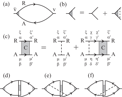
Figure 1: (a) Diagram for the Drude conductivity with (b) the vertex correction. (c) Bethe-Salpeter equation for the Cooperon propagator with valley indices $\xi\mu\xi^{\prime}\mu^{\prime}$ and AB lattice indices $\alpha\beta\alpha^{\prime}\beta^{\prime}$. (d) Bare ’Hikami box’ relating the conductivity correction to the Cooperon propagator with (e) and (f) dressed ’Hikami boxes’. Solid lines represent disorder averaged $G^{R/A}$, dashed lines represent disorder.

(b). The WL correction to the conductivity is associated with the disorder-averaged two-particle correlation function $C_{\alpha\beta,\alpha^{\prime}\beta^{\prime}}^{\xi\mu,\xi^{\prime}\mu^{\prime}}$ known as the Cooperon. It obeys the Bethe-Salpeter equation represented diagrammatically in Fig. 1(c). The shaded blocks in Fig. 1(c) are infinite series of ladder diagrams, while the dashed lines represent the correlator of the disorder in Eq. (4). Here, the valley indices ($\mathbf{K}_{\pm}$) of the Dirac-type electron are included as superscripts with incoming $\xi\mu$ and outgoing $\xi^{\prime}\mu^{\prime}$, and the sublattice ($AB$) indices as subscripts $\alpha\beta$ and $\alpha^{\prime}\beta^{\prime}$.

It is convenient to classify Cooperons in graphene as iso- and pseudospin singlets and triplets,

$$C_{s_{1}s_{2}}^{l_{1}l_{2}} = \frac{1}{4}\sum_{\alpha,\beta,\alpha^{\prime},\beta^{\prime},}\sum_{\xi,\mu,\xi^{\prime},\mu^{\prime},}\left(\Sigma_{y}\Sigma_{s_{1}}\Lambda_{y}\Lambda_{l_{1}}\right)_{\alpha\beta}^{\xi\mu}$$ (6)

$$\quad\times\,C_{\alpha\beta,\alpha^{\prime}\beta^{\prime}}^{\xi\mu,\xi^{\prime}\mu^{\prime}}\left(\Sigma_{s_{2}}\Sigma_{y}\Lambda_{l_{2}}\Lambda_{y}\right)_{\beta^{\prime}\alpha^{\prime}}^{\mu^{\prime}\xi^{\prime}}\,.$$

Such a classification of modes is permitted by the commutation of the iso- and pseudospin operators $\vec{\Sigma}$ and $\vec{\Lambda}$ in Eqs. (2,3,6), $[\Sigma_{s},\Lambda_{l}]=0$. To select the isospin singlet ($s=0$) and triplet ($s=x,y,z$) Cooperon components (scalar and vector representation of the group SU${}_{2}^{\Sigma}\equiv\{e^{ia\vec{n}\cdot\!\vec{\Sigma}}\}$), we project the incoming and outgoing Cooperon indices onto matrices $\Sigma_{y}\Sigma_{s_{1}}$and $\Sigma_{s_{2}}\Sigma_{y}$, respectively. The pseudospin singlet ($l=0$) and triplet ($l=x,y,z$) Cooperons (scalar and vector representation of the ’valley’ group SU${}_{2}^{\Lambda}\equiv\{\mathrm{e}^{ib\vec{n}\cdot\!\vec{\Lambda}}\}$) are determined by the projection of $C_{\alpha\beta,\alpha^{\prime}\beta^{\prime}}^{\xi\mu,\xi^{\prime}\mu^{\prime}}$ onto matrices $\Lambda_{y}\Lambda_{l_{1}}$ ($\Lambda_{l_{2}}\Lambda_{y}$) and are accounted for by superscript indices in $C_{s_{1}s_{2}}^{l_{1}l_{2}}$.

For disorder $\mathrm{\hat{I}}u(\mathbf{r})$, the equation in Fig. 1(c) is

$$C_{s_{1}s_{2}}^{l_{1}l_{2}}\left(\mathbf{q}\right)=\tau_{0}\,\delta^{l_{1}l_{2}}\delta_{s_{1}s_{2}}\\ +\,\frac{1}{4\pi\gamma\tau_{0}\hbar}\sum_{s,l}C_{ss_{2}}^{ll_{2}}\left(\mathbf{q}\right)\int\frac{d^{2}p}{\left(2\pi\right)^{2}}\\ \times\,\mathrm{Tr}\Big{\{}\Sigma_{s}\Sigma_{y}\Lambda_{l}\Lambda_{y}\left[\hat{G}_{\mathbf{p},\hbar\omega+\epsilon}^{R}\right]^{\mathrm{t}}\Lambda_{y}\Lambda_{l_{1}}\Sigma_{y}\Sigma_{s_{1}}\hat{G}_{\hbar\mathbf{q}-\mathbf{p},\epsilon}^{A}\Big{\}}.$$ (7)

It leads to a series of coupled equations for the Cooperon matrix $\mathbf{C}^{l}$ with components $C_{ss^{\prime}}^{ll}$. It turn out that for potential disorder $\mathrm{\hat{I}}u(\mathbf{r})$ isospin-singlet modes $C_{00}^{ll}$ are gapless in all (singlet and triplet) pseudospin channels, whereas triplet modes $C_{xx}^{ll}$ and $C_{yy}^{ll}$ have relaxation gaps $\Gamma_{x}^{l}=\Gamma_{y}^{l}=\frac{1}{2}\tau_{0}^{-1}$ and $C_{zz}^{ll}$ have gaps $\Gamma_{z}^{l}=\tau_{0}^{-1}$. When obtaining the diffusion equations for the Cooperons using the gradient expansion of the Bethe-Salpeter equation we take into account its matrix structure. The matrix equation for each set of four Cooperons $\mathbf{C}^{l}$,where $l=0,x,y,z$ has the form

$$\left(\begin{array}[]{cccc}\frac{1}{2}v^{2}\tau_{0}q^{2}+\Gamma_{0}^{l}-i\omega&\frac{-i}{2}vq_{x}&\frac{-i}{2}vq_{y}&0\\ \frac{-i}{2}vq_{x}&\frac{1}{2}\tau_{0}^{-1}&0&0\\ \frac{-i}{2}vq_{y}&0&\frac{1}{2}\tau_{0}^{-1}&0\\ 0&0&0&\tau_{0}^{-1}\end{array}\right)\mathbf{C}^{l}=\hat{1}.$$

After the isospin-triplet modes were eliminated, the diffusion operator for each of the four gapless/low-gap modes $C_{0}^{l}$ becomes $Dq^{2}-i\omega+\Gamma_{0}^{l}$, where $D=\frac{1}{2}v^{2}\tau_{\mathrm{tr}}=v^{2}\tau_{0}$.

Symmetry-breaking perturbations lead to relaxation gaps $\Gamma_{0}^{l}$ in the otherwise gapless pseudospin-triplet components, $C_{0}^{x},C_{0}^{y},C_{0}^{z}$ of the isospin-singlet Cooperon $C_{0}^{l}$, though they do not generate a relaxation of the pseudospin-singlet $C_{0}^{0}$ protected by the time-reversal symmetry of the Hamiltonian (4). We include all scattering mechanisms described in Eq. (4) in the corresponding disorder correlator (dashed line) on the r.h.s. of the Bethe-Salpeter equation and in the scattering rate in the disorder-averaged $G^{R/A}$, as $\tau_{\mathrm{0}}^{-1}\rightarrow\tau^{-1}=\tau_{\mathrm{0}}^{-1}+\sum_{sl}\tau_{sl}^{-1}$. For simplicity, we assume that different types of disorder are uncorrelated, $\langle u_{s,l}(\mathbf{r})u_{s^{\prime},l^{\prime}}(\mathbf{r}^{\prime})\rangle=u_{sl}^{2}\delta_{ss^{\prime}}\delta_{ll^{\prime}}\delta(\mathbf{r}-\mathbf{r}^{\prime})$ and, on average, isotropic in the $x-y$ plane: $u_{xl}^{2}=u_{yl}^{2}\equiv u_{\bot l}^{2}$, $u_{sx}^{2}=u_{sy}^{2}\equiv u_{s\bot}^{2}$. We parametrize them by scattering rates $\tau_{sl}^{-1}=\pi\gamma u_{sl}^{2}/\hbar$, where $\tau_{sx}^{-1}=\tau_{sy}^{-1}\equiv\tau_{s\bot}^{-1}$ and $\tau_{xl}^{-1}=\tau_{yl}^{-1}\equiv\tau_{\bot l}^{-1}$ due to the $x-y$ plane isotropy of disorder, which are combined into the intervalley scattering rate $\tau_{\mathrm{i}}^{-1}$ and the intra-valley rate $\tau_{\mathrm{z}}^{-1}$, as

$$\tau_{\mathrm{i}}^{-1}=4\tau_{\bot\bot}^{-1}+2\tau_{z\bot}^{-1},\;\;\tau_{\mathrm{z}}^{-1}=4\tau_{\bot z}^{-1}+2\tau_{zz}^{-1}.$$ (8)

The trigonal warping term, ${\hat{h}}_{\mathrm{w}}$ in the Hamiltonian (1) plays a crucial role for the interference effects since it breaks the $\mathbf{p}\rightarrow-\mathbf{p}$ symmetry of the Fermi lines within each valley: $\epsilon(\mathbf{K}_{\pm},-\mathbf{p})\neq\epsilon(\mathbf{K}_{\pm},\mathbf{p})$, while $\epsilon(\mathbf{K}_{\pm},-\mathbf{p})=\epsilon(\mathbf{K}_{\mp},\mathbf{p})$ kpoints . It has been noticed EggShaped that such a deformation of a Fermi line of 2D electrons suppresses Cooperons. As ${\hat{h}}_{\mathrm{w}}$ has a similar effect, it suppresses the pseudospin-triplet intravalley components $C_{0}^{x}$ and $C_{0}^{y}$, at the rate

$$\tau_{\mathrm{w}}^{-1}=2\tau_{0}\left(\epsilon^{2}\mu/\hbar v^{2}\right)^{2}.$$ (9)

However, since warping has an opposite effect on valleys $\mathbf{K}_{+}$ and $\mathbf{K}_{-}$, it does not cause gaps in the intervalley Cooperons $C_{0}^{0}$ (the only true gapless Cooperon mode) and $C_{0}^{z}$.

Altogether, the relaxation of modes $C_{0}^{l}$ can be described by the following combinations of rates:

$$\Gamma_{0}^{0}=0,\;\Gamma_{0}^{z}=2\tau_{\mathrm{i}}^{-1},\;\Gamma_{0}^{x}=\Gamma_{0}^{y}=\tau_{\mathrm{w}}^{-1}+\tau_{\mathrm{z}}^{-1}+\tau_{\mathrm{i}}^{-1}\equiv\tau_{\ast}^{-1}.$$

In the presence of an external magnetic field, $\mathbf{B}=\mathrm{rot}\mathbf{A}$ and inelastic decoherence, $\tau_{\varphi}^{-1}$, equations for $C_{0}^{l}\equiv$ $C_{00}^{ll}$ read

$$[D(i\mathbf{\nabla}+\tfrac{2e}{c\hbar}\mathbf{A)}^{2}+\Gamma_{0}^{l}+\tau_{\varphi}^{-1}-i\omega]C_{0}^{l}\left(\mathbf{r},\mathbf{\ r^{\prime}}\right)=\delta\left(\mathbf{r}-\mathbf{r^{\prime}}\right).$$

(c). Due to the momentum-independent form of the current operator $\mathbf{\tilde{v}=}2v\vec{\Sigma}$, the WL correction to conductivity $\delta g$ includes two additional diagrams, Fig. 1(e) and (f) besides the standard diagram shown in Fig. 1(d). Each of the diagrams in Fig. 1(e) and (f) [not included in the analysis in Ref.AndoWL ] produces a contribution equal to $(-\frac{1}{4})$ of that in Fig. 1(d). This partial cancellation, together with a factor of four from the vertex corrections and a factor of two from spin degeneracy leads to

$$\delta g=\frac{2e^{2}D}{\pi\hbar}\!\int\!\frac{d^{2}q}{\left(2\pi\right)^{2}}\left(C_{0}^{x}+C_{0}^{y}+C_{0}^{z}-C_{0}^{0}\right).$$ (10)

Using Eq. (10), we find the $B=0$ temperature dependent correction, $\delta\rho$ to the graphene sheet resistance,

$$\frac{\delta\rho\left(0\right)}{\rho^{2}}=-\delta g=\frac{e^{2}}{\pi h}\left[\ln(1+2\frac{\tau_{\varphi}}{\tau_{\mathrm{i}}})-2\ln\frac{\tau_{\varphi}/\tau_{\mathrm{tr}}}{1+\frac{\tau_{\varphi}}{\tau_{\ast}}}\right],$$ (11)

and evaluate magnetoresistance, $\rho(B)-\rho(0)\equiv$ $\Delta\rho(B)$,

$$\Delta\rho(T,B)=-\,\frac{e^{2}\rho^{2}}{\pi h}\left[F(\frac{B}{B_{\varphi}})-F(\frac{B}{B_{\varphi}+2B_{\mathrm{i}}})\right.$$

$$\;\;\;\;\;\;\;\;\;\;\;\;\;\;\;\;\;\;\;\;\;\;\left.-2F(\frac{B}{B_{\varphi}+B_{\ast}})\right],$$ (12)

$$F(z)=\ln z+\psi(\frac{1}{2}+\frac{1}{z}),\;B_{\varphi,\mathrm{i},\ast}=\frac{\hbar c}{4De}\tau_{\varphi,\mathrm{i},\ast}^{-1}\,.$$

Here, $\psi$ is the digamma function, and the decoherence $\tau_{\varphi}^{-1}(T)$ determines the MR curvature at $B\lesssim B_{\varphi}$.

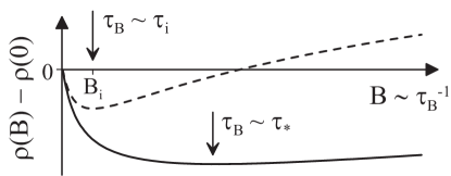
Figure 2: MR expected in a phase-coherent graphene $\tau_{\varphi}\gg\tau_{\mathrm{i}}$: with $\tau_{z},\tau_{\mathrm{w}}\gg\tau_{\mathrm{i}}$ (dashed) and $\tau_{\ast}\ll\tau_{\mathrm{i}}$ (solid line). In the case of $\tau_{\varphi}<\tau_{\mathrm{i}}$, $\delta\rho=0$, so that $\Delta\rho(B)=0$.

Equations (12) and (11) represent the main result of this paper. They show that in graphene samples with the intervalley time shorter than the decoherence time, $\tau_{\varphi}>\tau_{\mathrm{i}}$, the quantum correction to the conductivity has the WL sign. Such behavior is expected in graphene tightly coupled to the substrate (which generates atomically sharp scatterers). Figure 2 illustrates the corresponding MR in two regimes: $B_{\ast}\sim B_{\mathrm{i}}$ ($\tau_{z},\tau_{\mathrm{w}}\gg\tau_{\mathrm{i}}$) and $B_{\ast}\gg B_{\mathrm{i}}$ ($\tau_{\ast}\ll\tau_{\mathrm{i}}$). In both cases, the low-field MR, at $B<B_{\mathrm{i}}$ is negative (for $B_{\ast}\sim B_{\mathrm{i}}$, the MR changes sign at $B\sim B_{\mathrm{i}}$). A dashed line shows what one would get upon neglecting the effect of warping, the solid curve shows the MR behavior in graphene with a high carrier density, where the effect of warping is strong and leads to a fast relaxation of intravalley Cooperons, at the rate described in Eq. (9). Then, in Eqs. (11,12) $\tau_{\ast}\approx\tau_{\mathrm{w}}\ll\tau_{\mathrm{i}}<\tau_{\varphi}$ and $B_{\ast}\gg B_{\mathrm{i}}$, which determines MR of a distinctly WL type. Note that in the latter case MR is saturated at $B\sim B_{\mathrm{i}}$, in contrast to the WL MR in conventional electron systems, where the logarithmic field dependence extends into the field range of $\hbar c/4De\tau_{\mathrm{tr}}$. In a sheet loosely attached to a substrate (or suspended), the intervalley scattering time may be longer than the decoherence time, $\tau_{\mathrm{i}}>\tau_{\varphi}>\tau_{\mathrm{w}}$ ($B_{\mathrm{i}}<B_{\varphi}<B_{\mathrm{\ast}}$). In this case, $C_{0}^{z}$ in Eq. (10) is effectively gapless and cancels $C_{0}^{0}$, whereas trigonal warping suppresses the modes $C_{0}^{x}$ and $C_{0}^{y}$, so that $\delta g=0$ and MR displays neither WL nor WAL behavior: $\Delta\rho(B)=0$.

Equation (12) explains why in the recent experiments on the quantum transport in graphene DiscGeim the observed low-field MR displayed a suppressed WL behavior rather than WAL. For all electron densities in the samples studied in DiscGeim the estimated warping-induced relaxation time is rather short, $\tau_{\mathrm{w}}/\tau_{\mathrm{tr}}\sim 5\div 30$, $\tau_{\mathrm{w}}<\tau_{\varphi}$, which excluded any WAL. Moreover, the observation DiscGeim of a suppressed WL MR in devices with a tighter coupling to the substrate agrees with the behaviour expected in the case of sufficient intervalley scattering, $\tau_{\mathrm{i}}<\tau_{\varphi}$, whereas the absence of any WL MR, $\Delta\rho(B)=0$ for a loosely coupled graphene sheet is what we predict for samples with a long intervalley scattering time, $\tau_{\mathrm{i}}>\tau_{\varphi}$.

In a narrow wire with the transverse diffusion time $L_{\bot}^{2}/D\ll\tau_{\mathrm{i}},\tau_{\ast},\tau_{\varphi}$, edges scatter between valleys edge . Thus, we estimate $\Gamma_{0}^{l}\sim\pi^{2}D/L_{\bot}^{2}$ for the pseudospin triplet in a wire, whereas the singlet $C_{0}^{0}$ remains gapless. This yields negative magnetoresistivity for $B\lesssim 2\pi B_{\bot}$, $B_{\bot}\equiv\hbar c/eL_{\bot}^{2}$:

$$\frac{\Delta\rho_{\mathrm{wire}}\left(B\right)}{\rho^{2}}=\frac{2e^{2}L_{\varphi}}{h}\,\left[\frac{1}{\sqrt{1+\frac{1}{3}B^{2}/B_{\varphi}B_{\bot}}}-1\right].$$ (13)

Equations (11-13) completely describe the WL effect in graphene and explain how the WL magnetoresistance reflects the degree of valley symmetry breaking. They show that, despite the chiral nature of electrons in graphene suggestive of antilocalisation, their long-range propagation in a real disordered material or a narrow wire does not manifest the chirality.

We thank I.Aleiner, V.Cheianov, A.Geim, P.Kim, O.Kashuba, and C.Marcus for discussions. This project has been funded by the EPSRC grant EP/C511743.

References

(1) Y. Zheng, T. Ando, Phys. Rev. B 65, 245420
(2002); V. Gusynin, S. Sharapov, Phys. Rev. Lett. 95, 146801
(2005); A. Castro Neto, F. Guinea, N. Peres, Phys. Rev. B 73, 205408 (2006)
(2) T. Ando, T. Nakanishi, R. Saito, J. Phys. Soc. Japan
67, 2857 (1998)
(3) E. McCann and V.I Fal’ko, Phys. Rev. Lett. 96,
086805 (2006)
(4) V. Cheianov, V.I. Fal’ko, Phys. Rev. B 74,
041403 (2006)
(5) K.S. Novoselov et al., Nature 438, 197
(2005); K. Novoselov et al, Nature Physics 2, 177 (2006)
(6) Y. Zhang et al., Phys. Rev. Lett. 94,
176803 (2005); Y. Zhang et al., Nature 438, 201 (2005)
(7) T. Ando, J. Phys. Soc. Jpn. 74, 777 (2005)
(8) Here, , is the lattice constant.
(9) B.L. Altshuler, D. Khmelnitski, A.I. Larkin, P.A. Lee, Phys.
Rev. B 22, 5142 (1980)
(10) S. Hikami, A.I. Larkin, N. Nagaosa, Progr. Theor Phys.
63, 707 (1980)
(11) H. Suzuura, T. Ando, Phys. Rev. Lett. 89, 266603
(2002)
(12) D.V. Khveshchenko, Phys. Rev. Lett. 97, 036802
(2006)
(13) The group U4 can be described using 16 generators ; .
(14) In the basis [, , , ], time reversal of an operator is , and , , .
(15) E. Fradkin, Phys. Rev. B 33, 3257 (1986);
N. Shon, T. Ando, J. Phys. Soc. Jpn 67, 2421 (1998); E. McCann,
V. Fal’ko, Phys. Rev. B 71, 085415 (2005); M. Foster, A. Ludwig,
Phys. Rev. B 73, 155104 (2006)
(16) V. Fal’ko, T. Jungwirth, Phys. Rev. B 65,
081306 (2002); D. Zumbuhl et al, Phys. Rev. B 69, 121305
(2004)
(17) E. McCann and V.I. Fal’ko, J. Phys. Cond. Matt. 16,
2371 (2004)
(18) S. Morozov et al, Phys. Rev. Lett. 97,
016801 (2006)