Magnetization reversal through synchronization with a microwave

Abstract

Based on the Landau-Lifshitz-Gilbert equation, it can be shown that a circularly-polarized microwave can reverse the magnetization of a Stoner particle through synchronization. In comparison with magnetization reversal induced by a static magnetic field, it can be shown that when a proper microwave frequency is used the minimal switching field is much smaller than that of precessional magnetization reversal. A microwave needs only to overcome the energy dissipation of a Stoner particle in order to reverse magnetization unlike the conventional method with a static magnetic field where the switching field must be of the order of magnetic anisotropy.

Introduction–Magnetization reversal of single-domain magnetic nano-particles (Stoner particles)Hillebrands is of significant interest in magnetic data storage and spintronics. Finding an effective way to switch magnetization from one state to another depends on our basic understanding of magnetization dynamics. Magnetization can be manipulated by laserBigot , a polarized electric currentSlon ; current or a magnetic fieldHe . An important issue in magnetization reversal is the minimal switching field. Magnetization reversal using a static magnetic fieldHe ; Back ; Schum ; xrw or polarized electric currentSlon ; current has received close attention in recent years but there has been little investigation on microwave induced magnetization reversal. Thirion et al.grenoble made probably the first attempt in this direction. It was shown that a dramatic reduction of the minimal switching field is possible by applying a small radio-frequency (RF) field pulse (the decrease in the static field is much larger than the amplitude of the RF-field). In this paper, it is shown that a circularly-polarized microwave on its own can induce magnetization reversal. The minimal switching field depends on the microwave frequency. It can be shown that the minimal switching field is at a minimum at an optimal frequency. This optimal frequency is near the natural precession frequency at which the particle experiences the largest dissipation. At this optimal frequency, the switching field strength can be much smaller than the so-called Stoner-Wohlfarth (SW) limitStoner and precessional magnetization switching fieldHe ; Back ; Schum for a static magnetic field. Far from the optimal frequency, the switching field can be larger than the SW-limit.

The minimal switching field was first studied by Stoner and WohlfarthStoner . The SW-limit is the field at which the energy minimum around the initial state is destroyed and the target state is the only minimumHe ; Schum ; xrw ; Back , as illustrated in Fig. 1(a)-(b). In the absence of magnetic fields, two energy minima [$A$ and $B$ in Fig. 1(a)], separated by a potential barrier $\Delta E$, are along the easy-axis of a magnetic particle. At the SW-limit, the original minimum near the initial state $A$ disappears [Fig. 1(b)], and the particle will end up at its unique minimum near the target state $B$. Recent theoretical and experimental studiesHe ; Back ; Schum have shown that the minimal switching field could be smaller than the SW-limit. The reason has been explained earlierxrw . As illustrated in Fig. 1(c), magnetization reversal can occur even when the minimum around $A$ exists. The reversal can happen as long as the particle energy at $A$ is higher than that at the saddle point $SP$, and the particle can pass through $SP$ under its own dynamics. It can be shown that the minimal switching field is of the order of the potential barrier $\Delta E$xrw .

Figure 1: Energy surface of a uniaxial magnetic particle in various schemes. $SP$ denotes the saddle point between two minima. (a) In the absence of magnetic fields: $A$ and $B$ are the two minima, separated by a potential barrier $\Delta E$. (b) At the SW-limit: Target state $B$ is the only minimum. (c) Precessional magnetization reversal: The particle energy at $A$ is higher than that at $SP$ so that it can pass through $SP$ under its own dynamics. (d) New strategy: The system synchronizes its motion with a microwave, and climbs over the potential barrier to reverse its magnetization.

Fundamental differences between time-independent and time-dependent fields–The microwave induced magnetization reversal is fundamentally different from that of a static magnetic field because a static field is not an energy source whilst a microwave can. This can be seen from the dynamic equation governing the evolution of a single-domain magnetic nano-particle. For a particle with a magnetization of $\vec{M}=\vec{m}M_{s}$, $\vec{m}$ satisfies the Landau-Lifshitz-Gilbert (LLG) equationxrw ; Landau ,

$$(1+\alpha^{2})\frac{d\vec{m}}{dt}=-\vec{m}\times\vec{h}_{t}-\alpha\vec{m}\times(\vec{m}\times\vec{h}_{t}),$$ (1)

where $M_{s}$ is the saturated magnetization of the particle, and $\alpha$ is a dimensionless damping constant. The total field, measured in unit of $M_{s}$, comes from an applied magnetic field $\vec{h}$ and the internal effective field $\vec{h}_{i}$ due to the magnetic anisotropy $w(\vec{m},\vec{h})$, $\vec{h}_{t}=-\nabla_{\vec{m}}w(\vec{m},\vec{h})=\vec{h}_{i}+\vec{h}$. In Eq. (1), time $t$ is in unit of $(|\gamma|M_{s})^{-1}$ with $|\gamma|=2.21\times 10^{5}(rad/s)/(A/m)$ being the gyromagnetic ratio. From Eq. (1), the energy change rate for the particle can be obtainedxrw2

$$\frac{dw}{dt}=\vec{m}\cdot\dot{\vec{h}}-\frac{\alpha}{1+\alpha^{2}}|\vec{m}\times\vec{h}_{t}|^{2}.$$ (2)

The second term due to the damping is always negative, while the first term due to the external magnetic field can be either positive or negative if the field varies with time. Thus, a time-dependent magnetic field can be both energy source and energy sink.

New strategy–Having explained that a microwave can be an energy source, the synchronization phenomenon of nonlinear dynamic systemsszz can be used to reverse the magnetization of a Stoner particle by shining the particle with only a circularly polarized microwave. If the propagating direction of the microwave is along the particle’s easy-axis (the magnetic field rotates around the easy-axis with the microwave frequency), the particle’s magnetization in a synchronized motion precesses around the axis with the microwave frequency. As illustrated in Fig. 1(d), the magnetization starting from its initial minimum $A$ obtains energy from the microwave, and eventually reaches its synchronized state. If the synchronized state is over the saddle point $SP$ and on the side of minimum $B$, the magnetization reversal is realized when the microwave radiation is turned off because magnetization will end up at minimum $B$ through the usual ringing effectHe . It is known that a nonlinear dynamic system under an external periodic field may undergo a non-periodic motion other than synchronizationszz . In general, the reversal criterion is: The magnetization is reversed if the system can cross the saddle point $SP$ in Fig. 1.

To demonstrate the feasibility of the new strategy, an uniaxial magnetic anisotropy is considered,

$$w(\vec{m},\vec{h}=0)=-km_{x}^{2},$$ (3)

where $k>0$ measures the anisotropy strength. Without losing the generality, $k$ (used as a scale for the field strength according to Eq. (1)) shall be set to $1$. The easy-axis is chosen to be along the x-axis rather than the z-axis because the north and south poles are singular in spherical coordinates, and it is more convenient to locate the minima $A$ and $B$ (Fig. 1) away from the singularities.

Multiple synchronization solutions–Under a circularly-polarized microwave of amplitude $h_{0}$ and frequency $\omega$

$$\vec{h}(t)=h_{0}[\cos(\omega t)\hat{y}+\sin(\omega t)\hat{z}],$$ (4)

the synchronized motion is

$$\vec{m}(t)=\cos\eta\hat{x}+\sin\eta[\cos(\omega t+\varphi)\hat{y}+\sin(\omega t+\varphi)\hat{z}],$$ (5)

where $\eta$ (a constant of motion) is the precessional angle between $\vec{m}$ and the x-axis. $\varphi$ is the locking phase in the synchronized motion. Substitute Eqs. (3), (4), and (5) into Eq. (1), $\eta$ and $\varphi$ satisfy

$$\sin\eta\sqrt{\alpha^{2}\omega^{2}+(2-\omega/\cos\eta)^{2}}=h_{0},$$ (6)

$$\sin\varphi=-\alpha\omega\sin\eta/h_{0},$$ (7)

where $\eta\in[0,\pi]$. For fixed ($h_{0},\omega,\alpha$), $\eta$ and $\varphi$ may have multiple solutions. As illustrated in Fig. 2, the solutions of $\eta$ (solid lines) are plotted as a function of $h_{0}$ for $\omega=1$ and $\alpha=0.1$. The dashed lines denote the corresponding $\varphi$. Multiple solutions of $\eta,\varphi$ are evident. For example, there are 4 solutions of $\eta$ when $h_{0}\in[0.09,0.45]$. Numerically, it can be shown that two solutions around $\eta=1$ (in between) are unstable, while the other two near $\eta=0,\pi$ are stable. Thus, the system shall eventually end up at one of the two stable solutions. Which one the system will choose depends on the initial condition. For a given initial condition [$\vec{m}(0)=\hat{x}$ in this study], the system picks the solution near $\eta=\pi$ when $h_{0}$ is larger than a critical value called the minimal switching field. According to our reversal criterion, the magnetization is reversed through synchronization.

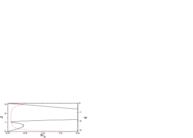
Figure 2: (color online) Graphic demonstration of multiple synchronization solutions. The solid lines are from Eq. (6) and the dashed lines are from Eq. (7). The graph is plotted at $\alpha=0.1$ and $\omega=1$.

Numerical verification of synchronized and non-synchronized motion–A nonlinear dynamic system under an external periodic field may undergo motion other than synchronized. Unfortunately, a non-synchronized motion is, in general, hard to define analytically. Usually, reliance must be placed on the numerical method. In terms of the LLG equation under a circularly-polarized microwave of Eq. (4), it is straight forwardxrw to calculate numerically $\vec{m}(t)$ starting from $\vec{m}(0)=\hat{x}$. The upper inset of Fig. 3 is the trajectory of $\vec{m}(t)$ after long time in $m_{x}m_{y}m_{z}$ space for $h_{0}=0.35;\omega=1;$ and $\alpha=0.1$. A simple closed loop in a plane parallel to the yz-plane indicates that this is a synchronized motion. Alternatively, the lower right inset of Fig. 3 is the long time trajectory of $\vec{m}(t)$ for $h_{0}=0.35;\omega=1.2;$ and $\alpha=0.1$. Its motion is very complicated, corresponding to a non-synchronized motion. It is found that whether the motion is synchronized or not it is sensitive to the microwave frequency. For example, all motions for $\omega=1$ are synchronized while both synchronized and non-synchronized motions are possible for $\omega=1.2$. The motion is non-synchronized for $h_{0}$ in the range of $[0.27,0.42]$ while it is synchronized for other values of $h_{0}$. Fig. 3 is $m_{x}$ of synchronized motions as a function of $h_{0}$ for $\omega=1$ and $1.2$.

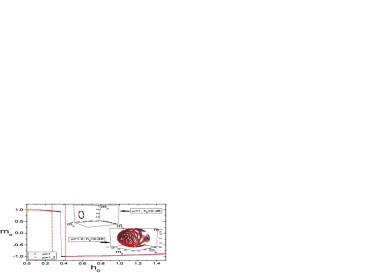
Figure 3: (color online) $m_{x}$ of synchronized motion vs. $h_{0}$ for $\alpha=0.1$ and $\omega=1$ (filled squares); $1.2$ (open circles). Non synchronized motion when $h_{0}\in[0.27,0.42]$ (between two dash-dotted lines) is found for $\omega=1.2$. Upper inset: Long time trajectory of $\vec{m}(t)$ for $\omega=1$ and $h_{0}=0.35$. Lower inset: Long time trajectory of $\vec{m}(t)$ for $\omega=1.2$ and $h_{0}=0.35$.

Optimal microwave frequency–Using the reversal criterion given earlier, it can be shown from Fig. 3, that the minimal switching field $h_{c}$ is about $0.375$ for $\omega=1$ because $m_{x}$ in the synchronized motion is negative when $h_{0}>h_{c}$. For $\omega=1.2$, the minimal switching field takes a value at which the magnetization undergoes a non-synchronized motion. Numerically, it can be shown that $\vec{m}$ crosses the yz-plane when $h_{0}\geq 0.285$. Thus, the minimal switching field is determined as $h_{c}=0.285$ for $\omega=1.2$. The reason that the value of the minimal switching field is so sensitive to the microwave frequency is because a switching field, as illustrated in Fig. 1(d), needs to overcome the dissipation which is related to the motion of the magnetization (see the LLG equation). To reveal the frequency dependence of the minimal switching field, Fig. 4 shows the minimal switching field $h_{c}$ vs. the microwave frequency $\omega$ for various $\alpha=0$; $0.001$; $0.1$; $1$; and $1.5$. $\omega=0$ corresponds to the case of a static field along the y-axis. The curve of $\alpha=0$ intersects the $h_{c}$-axis at $h_{c}=1$ which agrees with the exact minimal switching field $h_{c}=1$xrw . The intersections of all other curves of $\alpha\neq 0$, are the same as those with a static fieldHe ; xrw . When $\alpha\geq 1$, it becomes the SW-limit $h_{c}=2$. For a given $\alpha$, Fig. 4 shows the existence of an optimal microwave frequency, $\omega_{c}$, at which the minimal switching field is the smallest. Far from the optimal frequency, the minimal switching field can be larger than the SW-limit. The inset of Fig. 4 is $\omega_{c}$ vs. $\alpha$. The optimal frequency is near the natural precessional frequency at which the dissipation is a maximum.

Figure 4: (color online) The minimal switching field $h_{c}$ vs. $\omega$ for various damping constant $\alpha=0$; $0.001$; $0.1$; $1$; and $1.5$. Inset: The optimal frequency $\omega_{c}$ vs. $\alpha$.

Switching field as a function of dissipation–From above discussions, it can be seen that the minimal switching field is a minimum at the optimal frequency $\omega_{c}$. The squares symbols in Fig. 5 are the minimal switching fields at $\omega_{c}$ with different damping constant $\alpha$ for the uniaxial model of Eq. (3). They follow approximately the line of $h_{c}\approx 0.23+0.58\alpha$. This approximate linear relation is related to the fact that the damping (field) is proportional to $\alpha$. For comparisons, the minimal switching fields of a precessional magnetization reversal under a static magnetic field and the SW-limit are also plotted in Fig. 5. It can be seen that, for small damping, the smallest (at the optimal frequency) minimal switching field can be much smaller than that in the precessional magnetization reversal. For large damping, the switching field can be larger than the SW-limit.

Figure 5: $h_{c}$ vs $\alpha$ for the uniaxial model of Eq. (3) under different reversal schemes. Square symbols are the numerical results of $h_{c}$ at the optimal frequency in the present strategy with a circularly-polarized microwave. The dashed line is $h_{c}$ under a non-collinear static field of $135^{\circ}$ to the easy-axis. It saturates to the SW-limit beyond $\alpha=1$xrw .

Discussion and conclusions–It is important to compare the present strategy with other strategies involving time-dependent fields. Firstly, the current scheme is fundamentally different from that in the experiment of Thirion et al.grenoble in several aspects. 1) A circularly-polarized microwave of fixed frequencies is the only switching field in the new scheme. While in reference grenoble , a linear polarized RF field is used as an additional external field to reduce the main static switching magnetic field. 2) For a Co particle of $H_{i}=10^{5}A/m$Back , the optimal frequency is about order of $10GHz$ rather than GHz employed in reference grenoble . At $GHz$, Fig. 4 shows that the switching field would be too large to have any advantage over a static field. The current scheme is also very different from that in reference xrw2 in many aspects. 1) The time-dependent field in reference xrw2 is used as a ratchet that should be adjusted with the motion of magnetization. In contrast, the present scheme is based on the synchronization phenomenon in nonlinear dynamics such that a circularly-polarized microwave of fixed frequencies is used and the magnetization motion is synchronized with the microwave in the reversal process. 2) The switching field in reference xrw2 is in general non-monochromatic and very complicated, requiring a precise control of time-dependent polarization. Thus, it would be a great challenging to generate such a field. Alternatively, the current scheme is much easier to implement and it could be technologically important.

In conclusion, a circularly-polarized microwave induced magnetization reversal is proposed. The proposal is based on the facts that a microwave can constantly supply energy to a Stoner particle, and the magnetization motion can be synchronized with the microwave. It can be demonstrated that a Stoner particle under the radiation of a circularly-polarized microwave can indeed move out of its initial minimum and climb over the potential barrier. The switching field at the optimal microwave frequency will be much smaller than the SW-limit and that of the precessional magnetization reversal for small damping.

Acknowledgments–This work is supported by UGC, Hong Kong, through RGC CERG grants.

References

- (1) B. Hillebrands and K. Ounadjela, eds., Spin Dynamics in Confined Magnetic Structures I & II, (Springer-Verlag, Berlin, 2001).
- (2) M. Vomir, L.H.F. Andrade, L. Guidoni, E. Beaurepaire, and J.-Y. Bigot, Phys. Rev. Lett. 94, 237601 (2005).
- (3) J. Slonczewski, J. Magn. Magn. Mater. 159, L1 (1996); L. Berger, Phys. Rev. B 54 9353 (1996).
- (4) M. Tsoi et al., Phys. Rev. Lett. 80, 4281 (998); E. B. Myers, et al., Science 285, 867 (1999); J.A. Katine, et al., Phys. Rev. Lett. 84, 3149 (2000); J. Z. Sun, Phys. Rev. B 62, 570 (2000); Z. Li and S. Zhang, Phys. Rev. B 68, 024404 (2003); Y. B. Bazaliy, B. A. Jones and S. C. Zhang, Phys. Rev. B 57, R3213 (1998); 69, 094421 (2004).
- (5) L. He, W.D. Doyle, and H. Fujiwara, IEEE. Trans. Magn. 30, 4086 (1994); L. He, and W.D. Doyle, J. Appl. Phys. 79, 6489 (1996).
- (6) W.K. Hiebert, A. Stankiewicz, and M.R. Freeman, Phys. Rev. Lett. 79, 1134 (1997); C.H. Back, D. Weller, J. Heidmann, D. Mauri, D. Guarisco, E.L. Garwin, and H.C. Siegmann, Phys. Rev. Lett. 81, 3251 (1998); C.H. Back, R. Allenspach, W. Weber, S.S.P. Parkin, D. Weller, E.L. Garwin, and H.C. Siegmann, Science, 285, 864 (1999); Y. Acremann, C.H. Back, M. Buess, O. Portmann, A. Vaterlaus, D. Pescia, and H. Melchior, Science 290, 492 (2000).
- (7) H.W. Schumacher, C. Chappert, P. Crozat, R.C. Sousa, P.P. Freitas, J. Miltat, J. Fassbender, and B. Hillebrands, Phys. Rev. Lett. 90, 017201 (2003); H.W. Schumacher, C. Chappert, R.C. Sousa, P.P. Freitas, and J. Miltat, Phys. Rev. Lett. 90, 017204 (2003); T.M. Crawford, T.J. Silva, C.W. Teplin, and C.T. Rogers, Appl. Phys. lett. 74, 3386 (1999); M. Bauer, J. Fassbender, B. Hillebrands, and R. L. Stamps, Phys. Rev. B 61, 3410 (2000).
- (8) Z.Z. Sun, and X.R. Wang, Phys. Rev. B 71, 174430 (2005).
- (9) C. Thirion, W. Wernsdorfer, and D. Mailly, Nature Materials 2, 524 (2003).
- (10) E.C. Stoner, and E.P. Wohlfarth, Phil. Trans. Roy. Soc. London A240, 599 (1948).
- (11) L. Landau, and E. Lifshitz, Phys. Z. Sowjetunion 8, 153 (1953); T.L. Gilbert, Phys. Rev. 100, 1243 (1955).
- (12) Z.Z. Sun, and X.R. Wang, cond-mat/0511135.
- (13) Z.Z. Sun, H.T. He, J.N. Wang, S.D. Wang, and X.R. Wang, Phys. Rev. B 69, 045315 (2004); X.R. Wang, J.N. Wang, B.Q. Sun, and D.S. Jiang, Phys. Rev. B 61, 7261 (2000); X.R. Wang, and Q. Niu, Phys. Rev. B. 59, R12755 (1999).