Ground state cooling of atoms in optical lattices

Abstract

We propose two schemes for cooling bosonic and fermionic atoms that are trapped in a deep optical lattice. The first scheme is a quantum algorithm based on particle number filtering and state dependent lattice shifts. The second protocol alternates filtering with a redistribution of particles by means of quantum tunnelling. We provide a complete theoretical analysis of both schemes and characterize the cooling efficiency in terms of the entropy. Our schemes do not require addressing of single lattice sites and use a novel method, which is based on coherent laser control, to perform very fast filtering.

I Introduction

Ultracold atoms stored in optical lattices can be controlled and manipulated with a very high degree of precision and flexibility. This places them among the most promising candidates for implementing quantum computations OL_ent ; L_OL_QC_03 ; W_OL_QC_02 ; Bloch03 ; VC04 and quantum simulations of certain classes of quantum many–body systems CZ_OL_review ; Fermi-Hubbard ; OLspin ; JuanjoAKLT ; Kagome ; ringexchange ; ZollerPM ; LukinPM . However, both quantum simulation and quantum computation with this system face a crucial problem: the temperature in current experiments is too high. In this paper we propose and analyze two methods to decrease the temperature and thus to reach the conditions required to observe the interesting regimes in quantum simulations and quantum computation.

So far, several experimental groups have been able to load bosonic or fermionic atoms in optical lattices and reach the strong interaction regime Bloch02 ; Tonks ; ETH_Tonks ; ETH_Fermi ; NIST_OL_04 ; MIT_OL_Bose ; Texas_OL05 ; Grimm_OL_06 . In those experiments, the typical temperatures are still relatively high. For instance, the analysis of experiments in the Tonks gas regime indicates a temperature of the order of the width of the lowest Bloch band Tonks , and for a Mott Insulator a temperature of the order of the on-site interaction energy has been reported temp_Mott ; ETH_Tonks . For fermions one observes temperatures of the order of the Fermi energy temp_Fermi ; temp_Fermi_ETH ; ETH_Fermi_mol . Those temperatures put strong restrictions on the physical phenomena that can be observed with those systems and also on the quantum information tasks that can be carried out with them. They stem from the fact that atoms are loaded adiabatically starting from a Bose–Einstein condensate (in the case of bosons). On the one hand, the original condensate has a relatively high entropy BECStringari that is inherited by the atoms in the lattice in the adiabatic process. On the other hand, the process may not be completely adiabatic, which gives rise to heating. Thus, it seems that the only way of overcoming these problems is to cool the atoms once they have been loaded in the optical lattice.

One may think of several ways of cooling atoms in optical lattices. For example, one may use sympathetic cooling with a different Bose–Einstein condensate Fermi-Hubbard ; DFZ04 . Here we propose two alternative schemes which do not require the addition of a condensate. They aim at cooling atoms to the ground state of the Mott-insulating (MI) regime and allow us to predict temperatures which are low enough for practical interests. Our protocols are based on translation invariant operations (i.e. do not require single–site addressing) and include the presence of an additional harmonic trapping potential, as it is the case in present experiments. Although we will be mostly analyzing their effects on bosonic atoms, they can also be used for fermions.

The first scheme is based on the repeated application of occupation number filtering RZ03 . Via tunnelling, particles from the borders of the trap are transferred to the center, where they are discarded by subsequent filter operations. The second scheme combines filtering with algorithms inspired by quantum computation VC04 and hence will be termed algorithmic cooling of atoms NMR . The central idea is to split the atomic cloud into two components and to use particles at the border of one component as ”pointers” that remove ”hot” particles at the borders of the other component. We provide a detailed theoretical description of our cooling schemes and compare our theory with exact numerical calculations. In particular, we quantify the cooling efficiency analytically in terms of the initial and final entropy. We find that filtering becomes more efficient at low temperatures. This feature makes it possible to reach states very close to the ground state after only a few subsequent filtering operations. Our theory further predicts that the algorithmic protocol is more efficient at higher temperatures and that the final entropy per particle becomes zero in the thermodynamic limit. In addition, experimental requirements and time scales are discussed.

Since filtering is an important ingredient of all our protocols, we have devised an fast physical implementation which is based on optimal coherent laser control. Already comparatively simple optimization schemes work on a time scale that is significantly shorter than the one in RZ03 and Bloch_filter06 .

The paper is organized as follows. We start in Sect. II with reviewing the physical system in terms of the Bose-Hubbard model and discussing realistic initial state variables such as entropy and particle number. In Sect. III we give a detailed theoretical analysis of filtering under realistic experimental conditions. Building on this, we study in Sect. IV the repeated application of filtering. An algorithmic ground state cooling protocol is proposed and analyzed in Sect. V. Next, Sect. VI is dedicated to the discussion of our protocols, including a comparison of analytical results with numerical calculations. A further central result of our work is presented in Sect. VII. There we propose an ultra-fast implementation of filtering operations based on coherent laser control. We conclude with some remarks concerning possible variants and extensions of our protocols. In the Appendix we develop a fermionization procedure of the Bose-Hubbard Hamiltonian, which accounts for up to two particles per site.

II Initial state and basic concepts

We consider a gas of ultra-cold bosonic atoms which have been loaded into a three dimensional (3D) optical lattice. The lattice depth is proportional to the dynamic atomic polarizability times the laser intensity. We further account for an additional harmonic trapping potential which either arises naturally from the Gaussian density profile of the laser beams or can be controlled separately via an external magnetic or optical confinement Tonks ; Bloch05 .

In the following we will restrict ourselves to one-dimensional (1D) lattices, i.e. we assume that tunnelling is switched off for all times along the transversal lattice directions. This system is most conveniently described in terms of a single band Bose-Hubbard model oplat98 . For a lattice of length $L$ the Hamiltonian in second quantized form reads

$$H_{BH}=\sum_{k=-L/2}^{L/2}\left[-J(a^{\dagger}_{k}a_{k+1}+h.c.)+\frac{U}{2}n_{k}(n_{k}-1)+bk^{2}n_{k}\right].$$ (1)

The parameter $J$ denotes the hopping matrix element between two adjacent sites, $U$ is the on-site interaction energy between two atoms and the energy $b$ accounts for the strength of the harmonic confinement. Operators $a_{k}^{\dagger}$ and $a_{k}$ create and annihilate, respectively, a particle on site $k$, and $n_{k}=a^{\dagger}_{k}a_{k}$ is the occupation number operator. When raising the laser intensity the hopping rate decreases exponentially, whereas the interaction parameter $U$ stays almost constant oplat98 . Therefore we have adopted $U$ as the natural energy unit of the system.

In the following we will consider 1D thermal states in the grand canonical ensemble, which are characterized by two additional parameters, temperature $kT=1/\beta$ and chemical potential $\mu$. In particular, we are interested in the no-tunnelling limit comment_no-tunnel , $J\rightarrow 0$, in which the Hamiltonian (1) becomes diagonal in the Fock basis of independent lattice sites: $\{|n_{-(L-1)/2}\ldots n_{0}\ldots n_{(L-1)/2}\rangle\}$. The density matrix then factorizes into a tensor product of thermal states for each lattice site:

$$\rho=\frac{1}{\Theta}e^{-\beta(H_{BH}-\mu N)}=\bigotimes_{k=-L/2}^{L/2}\rho_{k},$$ (2)

which simplifies calculations considerably. For instance, the von-Neumann entropy can be written as,

$$S(\rho)={\rm tr}(\rho\log_{2}\rho)=\sum_{k}S(\rho_{k}).$$ (3)

This quantity will be central in this article, because it allows to assess the cooling performance of our protocols. To be more precise, we define two figures of merit. The ratio of the entropies per particle after and before invoking the protocol, $s_{f}/s_{i}$, quantifies the amount of cooling. The ratio of the final and initial number of particles, $N_{f}/N_{i}$, quantifies the particle loss induced by the protocol.

Note, however, that the entropy $S(\rho_{f})$ is only a good figure of merit if the state $\rho_{f}$ after the cooling protocol is close to thermal equilibrium. If this is not fulfilled, we compute an effective thermal state, $\rho_{f}\rightarrow\rho_{\textrm{eff}}$, by accounting for particle number and energy conservation in closed, isolated systems. This is performed numerically by tuning the chemical potential and temperature of a thermal state $\rho_{\textrm{eff}}$ until the expectation values for particle number and energy coincide with the ones of the original state $\rho_{f}$. This procedure can be implemented rather easily in the no-tunnelling regime, in which the density matrix factorizes (2).

Our figures of merit can then be calculated from $\rho_{\textrm{eff}}$. For instance, the final entropy is given by $S(\rho_{\textrm{eff}})$. It constitutes the maximum entropy of a state which yields the same expectation values for energy $E$ and particle number $N$ as the final state $\rho_{f}$. In this context it is important to point out that other variables, like energy or temperature, are not very well suited as figures of merit, because they depend crucially on external system parameters such as the harmonic trap strength.

We now study the structure of the initial state in more detail. To this end we first give typical parameter values. The analysis of recent experiments in the MI regime implies a substantial temperature of the order of the on-site interaction energy Tonks ; ETH_Tonks ; temp_Mott . This result is consistent with our own numerical calculations Cool2 and translates into an entropy per particle $s:=S/N\approx 1$. The particle number in a 1D tube of a 3D lattice as in Bloch02 typically ranges between $N=10$ and $N=130$ particles. A representative density distribution corresponding to such initial conditions (with $N=65$) is plotted in Fig. 1a. In this example the inverse temperature is given by $\beta U=4.5$. Since our cooling protocols lead to even lower temperatures, we will from now on focus on the low temperature regime, $\beta U\gg 1$. Moreover, we will only consider states with at most two particles per site, which puts the constraint $\mu\lesssim 2U-1/\beta$ on the chemical potential. Such a situation can either be achieved by choosing the harmonic trap shallow enough or by applying an appropriate filtering operation RZ03 .

Under the assumptions $e^{\beta U}\gg 1$ and $\mu-U/2\gtrsim b+1/(2\beta)$ we will now show that the density distribution of the initial state (2) can be separated into regions that are completely characterized by fermionic distribution functions of the form:

$$f_{k}(b,\beta,\mu)=\frac{1}{1+e^{\beta(bk^{2}-\mu)}}.$$ (4)

To be more precise, for sites at the borders of the density distribution, $bk^{2}\gg\mu-U/2+1/(2\beta)$, the mean occupation number is given by $\langle n_{k}\rangle\approx n_{\textrm{I}}(k)$ with $n_{\textrm{I}}(k):=f_{k}(b,\beta,\mu)$. In the center of the trap, $bk^{2}\ll\mu-U/2-1/(2\beta)$, one has: $\langle n_{k}\rangle\approx 1+n_{\textrm{II}}(k)$ with $n_{\textrm{II}}(k):=f_{k}(b,\beta,\mu_{\textrm{II}})$ and effective chemical potential $\mu_{\textrm{II}}:=\mu-U$ (see e.g. Fig. 1a).

Starting from state (2), with parameters $\beta$, $\mu$ and $b$, the grand canonical partition function for site $k$ is given by:

$$\Theta_{k}=1+a~{}x_{k}+b~{}x_{k}^{2},$$ (5)

with $x_{k}=e^{-\beta bk^{2}}$, $a=e^{\beta\mu}$ and $b=e^{\beta(2\mu-U)}$. In this notation the probabilities $p_{k}^{n}$ of finding $n$ particles at site $k$ can be written as: $p_{k}^{0}=1/\Theta_{k}$, $p_{k}^{1}=a~{}x/\Theta_{k}$ and $p_{k}^{2}=b~{}x^{2}/\Theta_{k}$. For analyzing these functions we split the lattice into a central region and two border regions. For lattice sites at the borders one finds $bx^{2}\ll 1,ax$, meaning that the probability for doubly occupied sites becomes negligible: $p_{k}^{2}\ll p_{k}^{0},p_{k}^{1}$. The average occupation is thus given by $\langle n_{k}\rangle\approx p_{k}^{1}$, with

$$p_{k}^{1}\approx\frac{ax}{1+ax}=\frac{1}{1+e^{\beta(bk^{2}-\mu)}}.$$ (6)

In the crossover region, $bk^{2}\approx\mu-U/2$, one obtains a MI phase ($p_{k}^{0},p_{k}^{2}\ll p_{k}^{1}\approx 1$). In the center of the trap one finds a negligible probability for empty sites: $p_{k}^{0}\ll p_{k}^{1},p_{k}^{2}$, since $ax,bx^{2}\gg 1$. The average population at site $k$ becomes $\langle n_{k}\rangle=p_{k}^{1}+2~{}p_{k}^{2}\approx 1+p_{k}^{2}$, where

$$p_{k}^{2}\approx\frac{bx^{2}}{ax+bx^{2}}=\frac{1}{1+e^{\beta(bk^{2}-(\mu-U))}}.$$ (7)

This is identical to the fermionic distribution (4) with effective chemical potential $\mu-U$. Hence the density distribution in this lattice region can be interpreted as a thermal distribution of hard-core bosons (phase II in Fig. 1a) sitting on top of a MI phase with unit filling. Note that this central MI phase is well reproduced by the function $n_{\textrm{I}}(k)$ , which originally has been derived for the border region. As a consequence, the density distribution for the whole lattice can be put in the simple form: $\langle n_{k}\rangle\approx n_{\textrm{I}}(k)+n_{\textrm{II}}(k)$, which corresponds to two fermionic phases I and II [Fig. 1a], sitting on top of each other. In other words, the initial state of our system can effectively be described in terms of non-interacting fermions, which can occupy two different energy bands I and II, with dispersion relations $\varepsilon_{\textrm{I}}=bk^{2}$ and $\varepsilon_{\textrm{II}}=bk^{2}+U$, respectively [see also Appendix A and PC05 ].

The initial density profile can be further characterized by two distinctive points. At sites $k=\pm k_{\mu}:=\sqrt{\mu/b}$, which correspond to the Fermi levels of phase I, one obtains $\langle n_{k_{\mu}}\rangle=1/2$. Hence, $k_{\mu}$ determines the radius of the atomic cloud. Note also that in the case $\mu\approx U$ singly occupied sites around the Fermi levels become degenerate with doubly occupied sites at the center of the trap. At the central site ($k=0$) one one finds an average occupation:

$$\langle n_{0}\rangle=1+\frac{1}{1+e^{\beta(U-\mu)}}.$$ (8)

For instance, the value $\langle n_{0}\rangle=3/2$ fixes the chemical potential to be $\mu=U$.

III Analysis of Filtering

By filtering we denote the state selective removal of atoms from the system, depending on the single site occupation number RZ03 . For instance, this can be achieved with a unitary operation

$$U_{m,0}^{M,m-M}:|m,0\rangle\leftrightarrow|M,m-M\rangle,$$ (9)

that transfers $m-M$ particles from a Fock state with $m$ atoms in internal states $|a\rangle$ to an initially unoccupied level $|b\rangle$. Particles in this level are removed subsequently and the process is repeated for all $m>M$. The maximum single site occupation number then becomes $M$. Alternatively, filtering can be described in terms of a completely positive map acting solely on the density operator of atoms $|a\rangle$:

$$F_{M} : \sum_{n,m}\rho_{n,m}|n\rangle\langle m|\to$$ (10)

$$\to\sum_{n,m\leq M}\rho_{n,m}|n\rangle\langle m|+\sum_{n>M}\rho_{n,n}|M\rangle\langle M|.$$

In particular, we are interested in the filtering operation $F_{1}$ which yields either empty or singly occupied sites. This operation can be carried out with the scheme introduced in RZ03 , which is based on the blockade mechanism due to atom–atom interactions. It enables a state selective adiabatic transfer of particles from one internal state of the atom to another. Recently, an alternative scheme which relies on resonant control of interaction driven spin oscillations has been put forward Bloch_filter06 . However, the predicted operation times of both approaches are comparatively long. Since fast filtering is crucial for the experimental realization of our protocols, we will propose in Sect. VII an ultra-fast, coherent implementation of $F_{1}$, relying on optimal laser control.

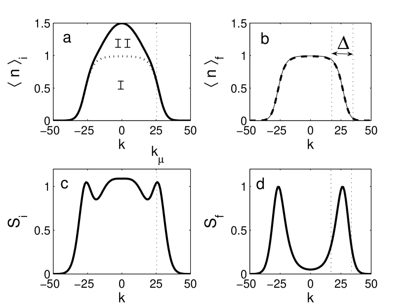
Figure 1: Spatial dependence of the average particle number $\langle n\rangle$ and entropy $S$ before (left) and after (right) the application of the filter operation $F_{1}$. The final particle distribution can be well described by Eq. (4) (dashed line in (b)). Numerical parameters for initial state: $N_{i}=65$, $s_{i}$=1 and $U/b=700$ ($\beta U=4.5$, $\mu/U=1$). Figures of merit: $s_{f}/s_{i}=0.56$ and $N_{f}/N_{i}=0.80$.

In Fig. 1 we study the action of $F_{1}$ on a realistic 1D thermal state in the no-tunnelling regime, as defined in the previous section. One observes that a nearly perfect MI phase with filling factor $\nu=1$ is created in the center of the trap. Defects in this phase are due to the presence of holes and preferably locate at the borders of the trap. This behavior is reminiscent of fermions, for which excitations can only be created within an energy range of order $kT$ around the Fermi level. This numerical observation can easily be understood with our previous analysis of the initial state. Filtering removes phase II, which is due to doubly occupied sites, and leaves the fermionic phase I unaffected [Fig. 1a].

Let us now study the cooling efficiency of operation $F_{1}$. This means we have to compute the entropy per particle of the states before and after filtering. According to our preceding discussion this problem reduces to the computation of the entropy $S$ and the particle number $N$, corresponding to the bands I and II. The entropy of a fermionic distribution of the form (4) is given by:

$$S_{F}(b,\beta,z) = \frac{1}{\sqrt{\beta b}}~{}\left[\sigma(z)\right.+\frac{\sqrt{\pi}}{2\ln 2}(2~{}\ln z~{}\textrm{Li}_{1/2}(-z)$$ (11)

$$- \left.\textrm{Li}_{3/2}(-z))\right],$$

with fugacity $z=e^{\beta\mu}$ and $\textrm{Li}_{n}(x)$ denoting the polylogarithm functions. The function $\sigma(z)$ is defined as the integral

$$\sigma(z):=\int_{-\infty}^{\infty}dx~{}\log_{2}\left(1+z~{}e^{-x^{2}}\right).$$ (12)

For phase I one can find a simpler expression for the entropy (11) by expansion around the Fermi level $k=k_{\mu}+dk$. Note that the range of validity, $|dk|\ll 1/\sqrt{\beta b}$, of this approximation covers all lattice sites that give a significant contribution to the total entropy. This yields the following relations:

$$S_{\textrm{I}}\approx\sigma_{\textrm{I}}\frac{2}{\beta\sqrt{b\mu}},\quad N_{\textrm{I}}\approx 2\sqrt{\frac{\mu}{b}},$$ (13)

with $\sigma_{\textrm{I}}:=\pi^{2}/(6\ln 2)$. For phase II this approach is typically not valid and one obtains the general expressions:

$$S_{\textrm{II}}=S_{F}(b,\beta,z_{\textrm{II}}),\quad N_{\textrm{II}}=-\sqrt{\frac{\pi}{\beta b}}~{}\textrm{Li}_{1/2}(z_{\textrm{II}}),$$ (14)

with $z_{\textrm{II}}=e^{\beta\mu_{\textrm{II}}}$. In the special case $\mu=U$ com_optimal one can simplify the above expressions to:

$$S_{\textrm{II}}\approx\sigma_{\textrm{II}}\frac{1}{\sqrt{\beta b}},\quad N_{\textrm{II}}\approx\eta_{\textrm{II}}\frac{1}{\sqrt{\beta b}},$$ (15)

with numerical coefficients $\sigma_{\textrm{II}}\approx 2.935$ and $\eta_{\textrm{II}}=(1-\sqrt{2})\sqrt{\pi}\zeta(1/2)\approx 1.063$.

With these findings we can now give a quantitative interpretation of Fig. 1. The initial entropy is composed of two components: $S_{i}=S_{\textrm{I}}+S_{\textrm{II}}$. Filtering removes the contribution $S_{\textrm{II}}$, which arises from the coexistence of singly and doubly occupied sites. The final entropy is thus given by $S_{f}=S_{\textrm{I}}$. This residual entropy is localized around the Fermi levels $-k_{\mu}$ and $k_{\mu}$ within a region of width $\Delta$ [Fig. 1]:

$$\Delta=\frac{2}{\beta\sqrt{b\mu}}=\frac{N_{\textrm{I}}}{\beta\mu},$$ (16)

and one can write $S_{f}=\sigma_{\textrm{I}}\ \Delta$. For the initial and final particle numbers one has the corresponding relations: $N_{i}=N_{\textrm{I}}+N_{\textrm{II}}$ and $N_{f}=N_{\textrm{I}}$. Hence, the final entropy per particle can be written as:

$$s_{f}=\frac{S_{f}}{N_{f}}\approx\sigma_{\textrm{I}}\frac{1}{\beta\mu}.$$ (17)

For the special choice $\mu=U$ (or equivalently $\langle n_{0}\rangle=1.5$) one finds the following expressions for our figures of merit:

$$\frac{s_{f}}{s_{i}} \approx \frac{\sigma_{\textrm{I}}}{\sqrt{\beta U}}\frac{\eta_{\textrm{II}}+2\sqrt{\beta U}}{\sigma_{\textrm{II}}\sqrt{\beta U}+2~{}\sigma_{\textrm{I}}},$$ (18)

$$\frac{N_{f}}{N_{i}} \approx \frac{1}{1+\frac{\eta_{\textrm{II}}}{2\sqrt{\beta U}}}.$$ (19)

This result shows that filtering becomes more efficient with decreasing temperature, since $s_{f}/s_{i}\propto 1/\sqrt{\beta U}\rightarrow 0$ and $N_{f}/N_{i}\rightarrow 1$ for $\beta U\rightarrow\infty$.

It is important to note that the state after filtering is not an equilibrium state, because it is energetically favorable that particles tunnel from the borders to the center of the trap, thereby forming doubly occupied sites. According to the discussion in the previous section this implies that the final entropy, which enters the cooling efficiency, should be calculated from an effective state $\rho_{eff}$ after equilibration. However, this would yield a rather pessimistic estimate for the cooling efficiency. Since the final density $n_{\textrm{I}}(k)$ already has the form of a thermal distribution function, one can easily come up with a much simpler (and faster) way to reach a thermodynamically stable configuration. While tunnelling is still suppressed, one has to decrease the strength of the harmonic confinement to a new value $b^{\prime}$, with $b^{\prime}\leq b~{}U/(2\mu)$. The system is then in the equilibrium configuration $f_{k}(b^{\prime},\beta^{\prime},\mu^{\prime})$ (4) with rescaled parameters $T^{\prime}=T~{}b^{\prime}/b$ and $\mu^{\prime}=\mu~{}b^{\prime}/b\leq U/2$. This observation shows that it is misleading to infer the cooling efficiency solely from the ratio $T^{\prime}/T$, because it depends crucially on the choice of $b^{\prime}$. Note also that this procedure indeed allows to achieve the predicted value (18) for the cooling efficiency.

IV Ground state cooling with sequential filtering

We have seen that filtering is limited by the fact that it cannot correct defects that arise from holes in a perfect MI phase. In order to circumvent this problem, we will now consider a repeated application of filtering, which will clearly profit from the increasing cooling efficiency as temperature is decreased. Our approach requires to iterate the following sequence of operations: (i) we allow for some tunnelling while the trap is adjusted adiabatically in order to reach a central occupation of $\langle n_{o}\rangle\approx 1.5$; (ii) we suppress tunnelling and perform the filtering operation $F_{1}$; (iii) the trap is slightly opened so that the final distribution resembles a thermal distribution of hard-core bosons. This way we transfer ”hot” particles from the borders to the center of the trap, where they can be removed by subsequent filtering.

We are interested in the convergence of the entropy and temperature as a function of the number of iterations. However, the adiabatic process is very difficult to treat both analytically and numerically. Therefore we distinguish in the following between three different scenarios that are based on specific assumptions.

(i) Thermal equilibrium: We assume that the entropy is conserved and that the system stays in thermal equilibrium throughout the adiabatic process. Since this condition will in general not be fulfilled for closed, isolated quantum systems, the following analysis can only provide a rather rough description of the real situation. To be more precise, we start from a thermal state with initial parameters $\beta$, $b$ and $\mu$. After filtering and adiabatic evolution one has a thermal state in the no-tunnelling regime with new parameters $\beta^{\prime}$, $b^{\prime}$ and $\mu^{\prime}$. As we have shown in the previous sections, thermal states in the no-tunnelling regime can effectively be described in terms of two fermionic components. This allows us to determine the new parameters $\beta^{\prime}$ and $b^{\prime}$ by identifying: $S_{\textrm{I}}(\beta,b)=S_{\textrm{I}}(\beta^{\prime},b^{\prime})+S_{\textrm{II}}(\beta^{\prime},b^{\prime})$ and $N_{\textrm{I}}(\beta,b)=N_{\textrm{I}}(\beta^{\prime},b^{\prime})+N_{\textrm{II}}(\beta^{\prime},b^{\prime})$. The desired central filling $\langle n_{0}\rangle=1.5$ fixes the chemical potentials to be $\mu=\mu^{\prime}=U$. Using expressions (13) and (15) one finds:

$$\beta^{\prime}U = \left(A+\sqrt{A^{2}+4\beta U}\right)^{2}/4,$$ (20)

$$\frac{b^{\prime}}{U} = \frac{b}{U}\left(1+\frac{\eta_{\textrm{II}}}{2\sqrt{\beta^{\prime}U}}\right),$$ (21)

with $A=(\sigma_{\textrm{II}}\beta U/\sigma_{\textrm{I}}-\eta_{\textrm{II}})/2$. After a second filtering operation the entropy per particle is thus given by:

$$s_{2}=\sigma_{\textrm{I}}\ \frac{1}{\beta^{\prime}U}.$$ (22)

Since our analysis only holds in the limit $\beta U\gg 1$, one can simplify the above expressions to: $\beta^{\prime}U\approx(\sigma_{\textrm{II}}\beta U/(2\sigma_{\textrm{I}}))^{2}$ and $b^{\prime}\approx b$. This allows us to establish a simple recursion relation for the entropy per particle $s_{n}$ after the $n$-th filter operation:

$$s_{n}\approx\frac{4\sigma_{\textrm{I}}}{\sigma_{\textrm{II}}^{2}}\ s_{n-1}^{2}.$$ (23)

Since the limit $\beta U\gg 1$ implies $s<1$, one finds that the entropy per particle converges extremely fast to zero.

(ii) Quantum evolution: Let us now study a more realistic situation. To this end we resort to an effective description of the quantum dynamics in terms of two coupled Fermi bands [Appendix A ]:

$$\tilde{H} = \sum_{k}\ [bk^{2}c_{k}^{\dagger}c_{k}+(bk^{2}+U)d_{k}^{\dagger}d_{k}$$ (24)

$$- J\ (c^{\dagger}_{k}c_{k+1}+\textrm{h.c.})$$

$$- \sqrt{2}J\ (c^{\dagger}_{k}d_{k+1}+d^{\dagger}_{k}c_{k+1}+\textrm{h.c.})$$

$$- 2J\ (d^{\dagger}_{k}d_{k+1}+\textrm{h.c.})].$$

Here, operators $c_{k},c_{k}^{\dagger}$ refer to energy band I and $d_{k},d_{k}^{\dagger}$ to band II, which is shifted from the lower band by the amount of the interaction energy $U$ (see Sect. II and Fig. 2). This treatment is self-consistent as long as the probability of finding a particle-hole pair is negligible, i.e. $\langle c_{k}c_{k}^{\dagger}d_{k}^{\dagger}d_{k}\rangle\approx 0$. In Sect. II we have shown analytically that this is indeed fulfilled for thermal states in the no-tunnelling regime and for low temperatures ($\beta U\gg 1$). We have checked that it also holds for thermal states at finite hopping rate $J$, provided that $J$ is not too big ($J\lesssim 0.5~{}U$). Since the Hamiltonian (24) is quadratic, we can study the complete protocol in terms of a single-particle picture. This can easily be done, if one further assumes that no level crossings occur in the course of the adiabatic evolution. Then, the state at any time $t$ can be computed by populating the single-particle energies of $\tilde{H}(t)$ according to the initial probabilities (after filtering) in energetically increasing order. This method is illustrated in more detail in Fig. 2.

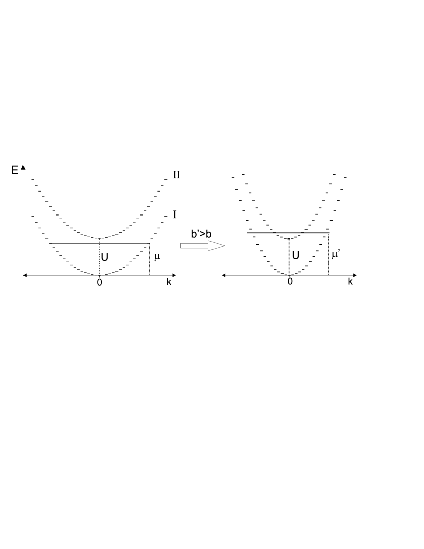
Figure 2: Effective description of thermal states in the no-tunnelling limit in terms of non-interacting fermions occupying two energy bands. The dispersion relations are $\varepsilon_{\textrm{I}}=bk^{2}$ and $\varepsilon_{\textrm{II}}=bk^{2}+U$, where $k$ denotes the lattice site and $U$ is the interaction energy. Increasing the harmonic trap strength from $b$ to $b^{\prime}$ increases the chemical potential to $\mu^{\prime}$ so that the population of the upper band becomes energetically favorable. In the bosonic picture this process corresponds to the formation of doubly occupied sites.

After the initial filtering step only states in the lowest energy band are occupied. The occupation probability is given by the fermionic distribution $f_{k}(b,\beta,\mu)$ (4). Increasing the trap strength to an appropriate value $b^{\prime}>b$ in the course of the adiabatic process makes it energetically favorable to occupy also the second band. We find the state after returning to the no-tunnelling regime, $\rho^{\prime}$, by populating the energy levels, corresponding to the new trap strength $b^{\prime}$, in energetically increasing order according to the initial probabilities $f_{k}(b,\beta,\mu)$. At this point we distinguish between two further scenarios: (ii.a) The state $\rho^{\prime}$ is mapped to a thermal state in the usual way by accounting for energy and particle number conservation [Sect. II]. This way we can quantify the amount of ”heating” resulting from the fact that the system is not in thermal equilibrium at the end of the adiabatic process due to the different structure of the energy spectrum. (ii.b) The next filtering operation acts directly on the time evolved state $\rho^{\prime}$.

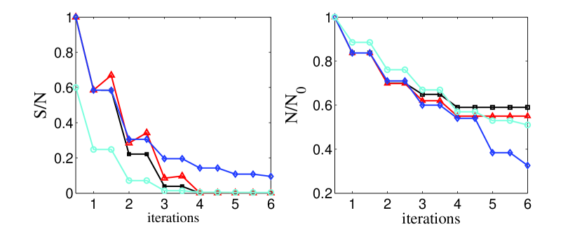
Figure 3: (Color online) Entropy per particle $S/N$ (left) and normalized number of particles $N/N_{0}$ (right) as a function of the number of filtering iterations for initially $N_{0}=100$ particles. As discussed in the text, we distinguish between the scenarios (i) (black line), (ii.a) (red line) and (ii.b) (blue and cyan).

Our results for all three cases are summarized in Fig. 3. We have computed numerically exact the entropy per particle as a function of the number of filtering cycles. Starting with an initial entropy $s_{0}=1$, scenarios (i) and (ii.a) predict that an entropy value close to zero can be obtained after only four iterations of the protocol . According to our underlying assumptions the system is in thermal equilibrium after each iteration of the protocol. In scenario (ii.b) the final entropy saturates at a finite value and the system is not in perfect thermal equilibrium. However, the final state still resembles a thermal state of hard-core bosons in a harmonic trap.

These results imply that sequential filtering can clearly profit from equilibration. The reason is that equilibration reduces the defect probability in the center of the lower band and transfers entropy to the upper band, where it can be removed subsequently. This process in combination with the increasingly high cooling efficiency of filtering at low temperatures can easily compensate the heating induced by the adiabatic quantum evolution. From our data we can deduce that this heating corresponds to an entropy increase of around 20 % com_heating . Without equilibration sequential filtering becomes very inefficient after the fourth iteration, which is also reflected in the excessive particle loss [Fig. 3]. The minimal attainable entropy is determined by the initial defect (hole) probability in the center of the trap. Starting from a much colder state, which exhibits almost unit filling in the center of the lower band, therefore yields a final state very close to the ground state [Fig. 3].

Remember that scenario (ii.b) is based on the assumption that no level crossings occur during the evolution. From our numerical analysis of the energy spectrum of (24) we know, however, that level crossings can indeed appear (see also Menotti ; Altman ). The reason is the vanishing small spatial overlap between single particle states at the border of the lower band and the center of the upper band. This has the following consequences for our previous analysis: For rather small particle numbers ($N\lesssim 15$) level crossings are rare and inter-band coupling occurs already for hopping rates, which are well within the range of validity of our single-particle description. We therefore expect that our predictions, as depicted in Fig. 3, are reasonable. For larger systems one has to tune the tunnelling rate deep into the superfluid regime $J\gtrsim 0.5~{}U$ in order to couple the two bands and to form doubly occupied sites. However, this regime is no longer accessible within our fermionic model (24). It remains to be investigated to what extent this will alter our predictions for the cooling efficiency of sequential filtering.

V Algorithmic ground state cooling

V.1 The protocol

We now propose a second cooling scheme, which we call algorithmic cooling, because it is inspired by quantum computation. As before the goal is to remove high energy excitations at the borders of the atomic cloud, which have been left after filtering. In contrast to sequential filtering we now restrict ourselves to a sequence of quantum operations that operate solely in the no-tunnelling regime. The central idea is to make use of spin-dependent lattices. A part of the atomic cloud can then act as a ”pointer” in order to address lattice sites which contain ”hot” particles. In this sense the scheme is similar to evaporative cooling, with the difference that an atomic cloud takes the role of the rf-knife. Another remarkable feature of the protocol is that the pointer is very inaccurate in the beginning (due to some inherent translational uncertainty in the system), but becomes sharper and sharper in the course of the protocol.

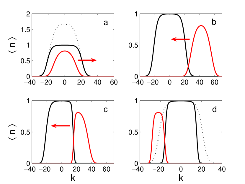
Figure 4: (Color online) Illustration of the protocol. The state is initialized with the filter operation $F_{2}$. (a) Particles from doubly occupied sites are transferred to state $|b\rangle$ (red) using operation $U_{2,0}^{1,1}$. (b) The lattice $|b\rangle$ has been shifted $2k_{\varepsilon}$ sites to the right, so that the two distributions barely overlap. (c) Density distribution after $k_{s}$ lattice shifts. After each shift doubly occupied sites have been emptied. Afterwards lattice $|b\rangle$ is shifted $4k_{\varepsilon}-k_{s}$ sites to the left and an analogous filter sequence is applied. (d) The final distribution of atoms in state $|a\rangle$ is sharper compared to the initial distribution (dotted). Numerical parameters: $N_{i}=65$, $s_{i}=1$, $U/b=300$, $k_{\varepsilon}$=21, $k_{s}=20$, $N_{f}=30.2$, $s_{f}=0.31$ (after equilibration).

The steps of this algorithmic protocol are: (i) We begin with a thermal equilibrium cloud with two or less atoms per site, all in internal state $|a\rangle$, and without hopping. This can be ensured with a filtering operation $F_{2}$. (ii) We next split the particle distribution into two, with an operation $U_{2,0}^{1,1}$ [Fig. 4a]. (iii) The two clouds are shifted away from each other until they barely overlap. Then we begin moving the clouds one against each other, emptying in this process all doubly occupied sites. This sequence sharpens the density distribution of both clouds. It is iterated for a small number of steps, of order $\Delta$ (16) [Fig. 4c]. (iv) The atoms of type $|b\rangle$ are moved again to the other side of the lattice and a process similar to (iii) is repeated [Fig. 4d]. (v) Remaining atoms in state $|b\rangle$ can now be removed.

The final particle distribution cannot be made arbitrarily sharp [Fig. 4d], due to the particle number uncertainty in the tails of the distribution. In the following we will consider this argument more rigorously and develop a theoretical description of the protocol.

V.2 Theoretical description

For the sake of simplicity we consider a slightly modified version of the protocol. The particle distributions $|a\rangle$ and $|b\rangle$ are now two identical but independent distributions of hard-core bosons of the form (4) Comment_theory .

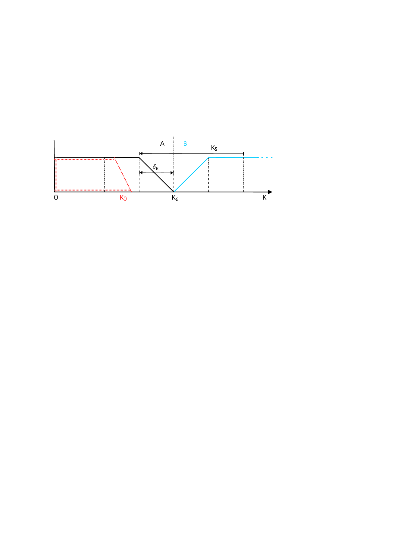
Figure 5: (Color online) Schematic description of the initial state for lattice sites $k\geq 0$: Two identical density distributions for hard-core bosons, belonging to different species A (black) and B (blue), are shifted $2k_{\varepsilon}$ lattice sites apart. The region of non-integer filling has width $\delta_{\varepsilon}$. In the course of the protocol the lattice of species B is shifted $k_{s}=3\delta_{\varepsilon}$ sites to the left.

The lattice $|b\rangle$ is shifted $2k_{\varepsilon}$ sites to the right. For given $\varepsilon$ the value $k_{\varepsilon}=\sqrt{\mu/b}\sqrt{1-\ln\varepsilon/\beta\mu}$ is chosen such that for atoms $|a\rangle$ it holds $\langle n^{a}_{k_{\varepsilon}}\rangle=\varepsilon$. This initial situation is depicted schematically in Fig. 5. The cutoff $\varepsilon$ defines also the width of the region with non-integer filling:

$$\delta_{\varepsilon}=\sqrt{\mu/b}\left(\sqrt{1-\ln\varepsilon/\beta\mu}-\sqrt{1+\ln\varepsilon/\beta\mu}\right).$$ (25)

We analyze first a protocol that involves $k_{s}=3\delta_{\varepsilon}$ lattice shifts and after each shift doubly occupied sites are emptied. Our goal is to compute the final shape of the density profile of atoms in state $|a\rangle$ (red line in Fig. 5). It is sufficient to consider only the reduced density matrices $\hat{\rho}_{a}$ and $\hat{\rho}_{b}$, which cover the range $k\in[k_{\varepsilon}-2\delta_{\varepsilon};k_{\varepsilon}]$ and $k\in[k_{\varepsilon};k_{\varepsilon}+2\delta_{\varepsilon}]$, respectively. These density matrices can be written in terms of convex sums over particle number subspaces:

$$\hat{\rho}_{a} = \sum_{N_{a}=0}^{2\delta_{\varepsilon}}p_{a}(N_{a})\hat{\rho}_{a}(N_{a}),$$ (26)

$$\hat{\rho}_{b} = \sum_{N_{b}=0}^{2\delta_{\varepsilon}}p_{b}(N_{b})\hat{\rho}_{b}(N_{b}).$$ (27)

The further discussion is based on the following central observation. If a state $\hat{\rho}_{a}(N_{a})$ interacts with a state $\hat{\rho}_{a}(N_{b})$ then our protocol produces a perfect MI state $\hat{\rho}^{\prime}_{a}(N^{\prime}_{a})$ composed of $N^{\prime}_{a}=(N_{a}-N_{b})/2$ particles. The factor $1/2$ arises from the fact that $k_{s}$ lattice shifts remove at most $k_{s}/2$ particles from distribution $|a\rangle$. Note that this relation also allows for negative particle numbers, because $N^{\prime}_{a}$ merely counts the number of particles on the right hand side of the reference point $k_{0}=k_{\varepsilon}-3/2\delta_{\varepsilon}$. The final density matrix after tracing out particles in $|b\rangle$ can then be written as a convex sum over nearly perfect (up to the cutoff error $\varepsilon$) MI states

$$\hat{\rho}^{\prime}_{a}=\sum_{N^{\prime}_{a}=-\delta_{\varepsilon}/2}^{\delta_{\varepsilon}/2}p^{\prime}_{a}(N^{\prime}_{a})\hat{\rho}^{\prime}_{a}(N^{\prime}_{a}),$$ (28)

with probabilities

$$p^{\prime}_{a}(N^{\prime}_{a})\simeq 2\sum_{N_{b}=\delta_{\varepsilon}}^{2\delta_{\varepsilon}}p_{a}(2N^{\prime}_{a}+N_{b})p_{b}(N_{b}).$$ (29)

The factor two is due to the fact that states with $N_{a}-N_{b}=2M$ and $N_{a}-N_{b}=2M+1$ are collapsed on the same MI state with $N_{a}^{\prime}=M$. Since Lyapounov’s condition CLT holds in our system, we can make use of the generalized central limit theorem and approximate $p_{a}(N)=p_{b}(N)$ by a Gaussian distribution with variance $\sigma^{2}=\delta N^{2}=\Delta/4=1/(2\beta\sqrt{b\mu})$. Evaluation of Eq. (29) then yields a Gaussian distribution with variance $\sigma^{\prime 2}=\sigma^{2}/2$. Since MI states do not contain holes, one can infer the final density distribution $\langle n^{a}_{k}\rangle^{\prime}$ directly from $p_{a}^{\prime}(N)$ by simple integration. This distribution can then be approximated by the (linearized) thermal distribution:

$$\langle n_{k}\rangle^{\prime}\simeq\frac{1}{1+e^{4(k-k_{0})/\Delta^{\prime}}}.$$ (30)

The new effective tail width $\Delta^{\prime}=\sqrt{\Delta\pi}/2$ of the distribution is roughly the square root of the original width $\Delta$ (16). This effect leads to cooling, which we will now quantify in terms of the entropy.

When applying similar reasoning also to the left side of distribution $|a\rangle$ one ends up with a mixture of MI states, which differ by their length and lateral position. This results in an extremely small entropy of the order $S_{\textrm{MI}}\sim\log_{2}{\Delta}$. However, this final state is typically far from thermal equilibrium. In order to account for a possible increase of entropy by equilibration, we have to compute the entropy of a thermal state, which has the same energy and particle number expectation values as the final state. In our case this is equivalent to computing the entropy directly from the density distribution (30):

$$S^{\prime}\approx\sigma_{\textrm{I}}~{}\Delta^{\prime}=\frac{\sigma_{\textrm{I}}\sqrt{\pi}}{\sqrt{2}}\frac{1}{(\beta^{2}b\mu)^{1/4}}=\frac{\sqrt{\pi}}{2}\frac{\sqrt{\beta\mu}}{\sqrt{N}}\ S,$$ (31)

where $N=N_{\textrm{I}}$ and $S=S_{\textrm{I}}$ (13) correspond to the expectation values after the initial filtering operation. The final particle number is given by: $N^{\prime}\simeq 2k_{0}\approx N(1+\ln\varepsilon/\beta\mu)$.

A significant improvement can be made by shifting the clouds only $k_{s}=2\delta_{\varepsilon}$ sites. This prevents inefficient particle loss, which has been included in our previous analysis in order make the treatment exact. With this variant the final particle number increases to $N^{\prime\prime}=2~{}(k_{\varepsilon}-\delta_{\varepsilon})$, while in good approximation the final entropy is still given by $S^{\prime}$. Hence, the final entropy per particle can be lowered to:

$$s^{\prime}=\frac{S^{\prime}}{N^{\prime\prime}}\approx\frac{\sqrt{\pi}}{2}~{}\frac{\sqrt{\beta\mu}}{1+\frac{\ln\varepsilon}{2\beta\mu}}~{}\frac{1}{\sqrt{N}}\ s.$$ (32)

This expression, which holds strictly only in the limit $\beta U\gg 1$, shows that for fixed $N$ the ratio $s^{\prime}/s$ becomes smaller at higher temperatures. Even more important, for fixed $\beta U$, the entropy per particle $s^{\prime}$ decreases with $1/\sqrt{N}$ as the initial number of particles in the system increases.

Finally, let us remark that the final entropy can be further reduced, when the protocol is repeated with two independent states of the form (28). In practice, this could be achieved with an ensemble of non-interacting atomic species in different internal levels. According to Eq. (29), each further iteration of the protocol decreases the total entropy by a factor $1/\sqrt{2}$.

VI Discussion of results

Let us now discuss and compare our previous results. In particular, we are interested in checking the range of validity of our analytical results by comparison with exact numerical calculations. To this end, we fix two parameters, $b/U$ and $\mu/U$, and compute the entropy per particle as a function of the inverse temperature $\beta U$ [Fig. 6].

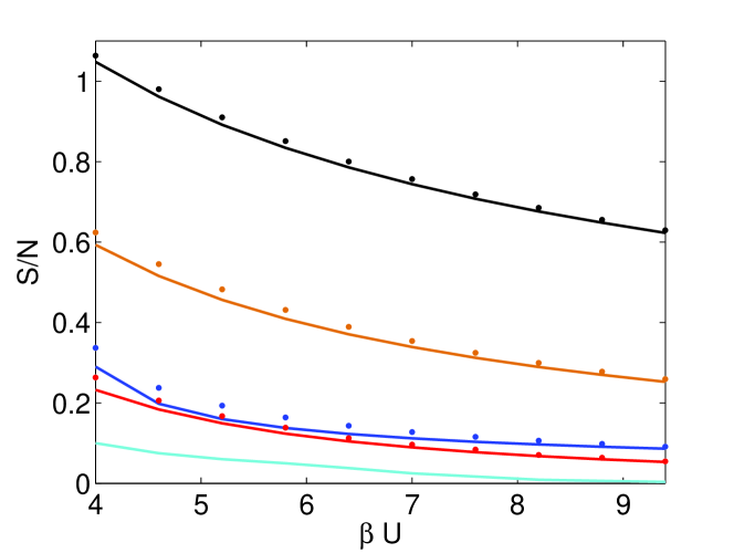
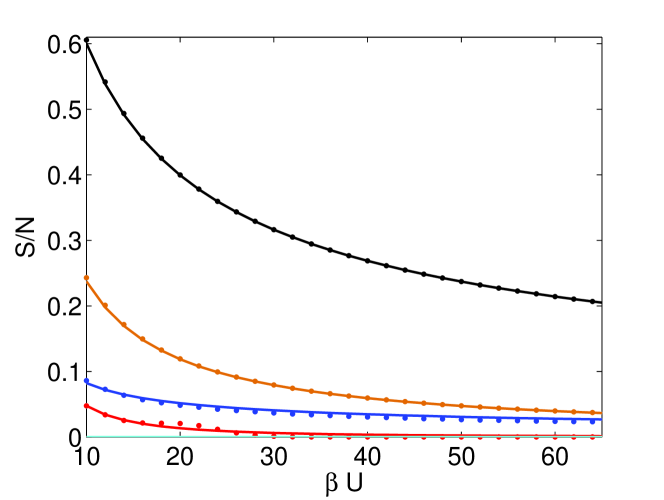
Figure 6: (Color online) Analytical (solid) and numerical (dots) results for the entropy per particle $s=S/N$ versus the inverse temperature $\beta U$ for fixed trap strength $b/U=1/2500$ and fixed $\mu=U$. We plot the initial value (black line) and the values after filtering with $F_{1}$ (Eq. (17), brown line). This is compared to more elaborate cooling protocols: entropy after two iterations of sequential filtering including equilibration (Eq. (22), red line), minimal entropy after sequential filtering without equilibration (cyan), and entropy after algorithmic cooling (Eq. (32), blue line). For the algorithmic protocol we have chosen $\varepsilon=0.03$ and $k_{s}=2~{}\delta_{\varepsilon}$. Note that this protocol creates classical correlations between lattice sites. The numerics are therefore based on a representation of classical density matrices in terms of matrix-product states Cool2 .

Our results can be summarized as follows. Firstly, we find that our theoretical description is very accurate in the low temperature limit $\beta U\gg 1$, and even holds in the (relatively) high temperature range $\beta U\gtrsim 1$. Secondly, our algorithmic protocol outperforms filtering considerably, especially in the high temperature range. Finally, based on the assumptions that underlie our calculations, subsequent filtering is typically superior to algorithmic cooling with respect to the minimal achievable entropy.

We now discuss advantages, experimental requirements and time scales of our cooling protocols.

VI.1 Sequential filtering

(i) Advantages: If one combines filtering with equilibration then the entropy per particle converges very fast to zero with the number of filter steps. The minimal value is only limited by finite size effects. Without equilibration, the minimal entropy is limited by the finite probability of finding a hole in the central MI phase of the initial distribution. Furthermore, sequential filtering naturally allows for cooling in a 3D setup, because it preserves spherical symmetry. Note that filtering, and hence sequential filtering, can also be applied to fermionic atoms in an optical lattice RZ03 .
(ii) Requirements and limitations: The repeated creation of doubly occupied sites in the center of the trap requires precise control of the harmonic confinement over a wide range of values. In addition, non-adiabatic changes of lattice and external potentials might induce heating, which could reduce the cooling efficiency considerably.
(iii) Time scales: The limiting factor here is not filtering but the adiabaticity criterion for changes of the hopping rate and the harmonic confinement. We have shown that after filtering the density distribution can be identified with a thermal distribution of spin-less fermions. Hence it is possible to find estimates for adiabatic evolution times based on single particle eigenfunctions, as calculated in Menotti . In the MI regime particle transfer from the borders to the center of the trap is very unlikely, because the eigenfunctions of the upper and lower Fermi band do not overlap. Therefore, we propose as a first step to decrease the lattice potential at fixed harmonic confinement until eigenfunctions start overlapping. This process can still be treated within a fermionic (or Tonks gas) picture, since only the lower band is populated [Fig. 2]. The average energy spacing around the Fermi level is $\overline{\delta E}=bN\approx 2~{}U/N$ in the no-tunnelling regime, and stays roughly constant when passing over to the tunnelling regime Menotti . As a consequence, the lattice potential should be varied on a time scale $T\gg h/\overline{\delta E}\approx 10$ ms for $N=50$ and $h/U=396~{}\mu$s WB04 . For the second process, which involves the change of the harmonic potential at fixed hopping rate, it is more difficult to make analytic predictions for adiabatic time scales, since our single-particle description (24) is no longer justified in general. One can, however, obtain a lower bound by considering the energy spectrum after returning to the no-tunnelling regime [Fig. 2]. The average energy spacing around the Fermi level is now dominated by the energy spacing at the bottom of the upper band: $\overline{\delta E^{\prime}}=\sqrt{b^{\prime}/\beta}/2\approx U/(N\sqrt{\beta U})$. This implies adiabatic evolution times which are a factor $\sqrt{\beta U}/2$ larger than for the first process. We have also verified the whole process numerically, using the matrix-product state representation of mixed states DMRGmixed . For initially $N=11$ particles we find adiabatic evolution times of the order $T\sim 30~{}\hbar/U$ for the first process, which is consistent with our analytical estimate. The second process is more time consuming with $T\gtrsim 120~{}\hbar/U$.

VI.2 Algorithmic cooling

(i) Advantages: The algorithmic protocol operates solely in the no-tunnelling regime. Adiabatic changes of the lattice and/or the harmonic potential, which are time consuming and might induce heating, are therefore not required. Moreover it does not demand arbitrary control over the harmonic confinement. The correct initial conditions can always be generated by the filter operation $F_{1}$. The protocol is more efficient in the high temperature range and for large particle numbers. Additionally to ground state cooling, the algorithm can be used to generate an ensemble of nearly perfect quantum registers for quantum computation. This state, which can also be considered as an ensemble of possible ground states in the uniform system, might already be sufficient for quantum simulation of certain spin Hamiltonians. Finally note that this protocol can naturally be applied also to fermionic systems.
(ii) Requirements and limitations: The heart of the protocol is the existence and control of spin-dependent lattices. Moreover, the algorithm is explicitly designed for cooling in one spatial dimension. Generalizations to higher dimensions are possible, but will typically not preserve the spherical symmetry of the initial density distribution. Moreover, one should keep in mind that the final states are typically far from thermal equilibrium.
(iii) Time scales: Adiabatic lattice shifts can be performed very fast on a time scale determined by the on-site trapping frequency $\nu\simeq 30$ kHz. The limiting factor is the number of filter operations, which is of the order $\delta_{\varepsilon}$ (25). Under realistic conditions this can amount to 50 operations. Filter operation times based on the adiabatic scheme RZ03 are of the order $T_{F}\sim 200~{}\hbar/U$. With $h/U=396~{}\mu$s WB04 one finds a total operation time $T\sim 630~{}$ ms, which is comparable with the typical particle life time in present setups using spin-dependent lattices Bloch03 . We have studied this problem with an alternative implementation of filtering [Sect. VII], which allows to reduce operation times by a factor of $\sim 15$, and hence makes algorithmic cooling feasible in current experimental setups.

VII Ultra-fast filtering scheme

We now propose an ultra-fast, coherent implementation of filtering, which is based on optimal laser control. We restrict our discussion to the filtering operation $F_{1}$ which is most relevant for our cooling protocols discussed above. We consider atoms in a particular internal level, $|a\rangle$, which are coupled to a second internal level, $|b\rangle$, via a Raman transition with Rabi frequency $\Omega(t)$. In contrast to the adiabatic scheme RZ03 we consider constant detuning, but vary $\Omega(t)$ in time. The Hamiltonian for a single lattice site reads

$$\hat{H} = \frac{U_{a}}{2}\hat{n}_{a}(\hat{n}_{a}-1)+U_{ab}\hat{n}_{a}\hat{n}_{b}+\frac{U_{b}}{2}\hat{n}_{b}(\hat{n}_{b}-1)$$ (33)

$$-(\Omega(t)\hat{a}^{\dagger}\hat{b}+\Omega^{*}(t)\hat{b}^{\dagger}\hat{a}),$$

where $U_{a}$, $U_{b}$ and $U_{ab}$ denote the on-site interaction energies, according to the different internal states. Note that $\Omega(t)$ can be complex, thus allowing for time-dependent phases. Our goal is to populate state $|a\rangle$ with exactly one particle per site which can be expressed by the unitary operation $U_{0}:|N,0\rangle\rightarrow|1,N-1\rangle,\ \forall\ N\in\{1,2,\ldots,N_{max}\}$. In order to do this, we control the time-dependence of $\Omega(t)$ coherently and in an optimal way. To be more precise, we optimize a sequence of $M$ rectangular shaped pulses of equal length:

$$\Omega(t)=\sum_{l=1}^{M}\Omega_{l}\times[\theta(t-t_{l})-\theta(t-t_{l+1})].$$ (34)

After time $T$ the system has evolved according to the unitary operator $U(T)$. We want to minimize the deviation of $U(T)$ from the desired operation $U_{0}$, which we quantify by the infidelity $\epsilon(T)=\sum_{N=1}^{N_{max}}\epsilon_{N}$, where $\epsilon_{N}=1-|\langle 1,N-1|U(T)|N,0\rangle|$. Since we allow for complex Rabi frequencies, $\epsilon(T)$ is a function of $2M$ parameters $\{\Omega_{l},\Omega_{l}^{*}\}$ with $l=1,\ldots,M$. For given $M$ and time $T$ we optimize the cost function $\epsilon(T)$ numerically using the Quasi-Newton method with a mixed quadratic and cubic line search procedure. This is repeated for different times $T$, while keeping the number of pulses $M$ constant. We then increase $M$ and repeat the whole procedure in order to check convergence of our results.

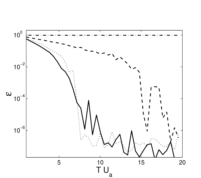
Figure 7: Operation error $\epsilon$ vs. time $tU_{a}$ for different interaction energies: $U_{b}=0.2U_{a}$, $U_{ab}=0.2U_{a}$, $\delta=0.8$ (solid); $U_{b}=U_{a}$, $U_{ab}=0.6U_{a}$, $\delta=0.8$ (dashed); $U_{b}=U_{a}$, $U_{ab}=0.2U_{a}$, $\delta=1.6$ (dotted); $U_{b}=U_{a}=U_{ab}$, $\delta=0$ (dashed-dotted). We optimize a sequence of $M=10$ pulses (34).

In Fig. 7 we plot the minimal error $\varepsilon(T)$ for different interaction strengths. Already for our simple control scheme we obtain very small errors, $\epsilon\sim 10^{-4}$, for a time $T\approx 7/U_{a}$ and interactions $U_{ab}=U_{b}=0.2U_{a}$. In comparison, the adiabatic scheme RZ03 would require $T\approx 150/U_{a}$ for the same set of parameters. However, in deep contrast to RZ03 our method works for a very broad range of interaction energies and in addition allows for very high fidelities.

It is important to remark that the operation time increases for small interaction anisotropies $\delta=|U_{a}+U_{b}-2U_{ab}|/U_{a}$ and for $\delta=0$ our method fails. In the special case $U_{a}=U_{b}=U_{ab}$ this follows from the fact that in the Hamiltonian (33) the interaction part commutes with the coupling part. These problems can be solved, either by displacing the lattices that trap atoms $|a\rangle$ and $|b\rangle$ and thereby reducing the effective interaction, $U_{ab}$, or by performing more elaborate controls than the one from Eq. (34).

VIII Conclusion

We have given a detailed analytical analysis of filtering in the no-tunnelling regime and in the presence of a harmonic trap. We have found that the residual entropy after filtering is localized at the borders of the trap, quite similar as in fermionic systems. Inspired by this result we have proposed two protocols that aim at removing particles from the borders and thus lead to cooling. One scheme transfers particles from the borders to the center of the trap, where they can be removed by subsequent filtering. In the other, algorithmic protocol particles from the system itself take the role of the rf-knife in evaporative cooling and remove directly particles at the borders. We have quantified the cooling efficiency of these protocols analytically in terms of the initial and final entropy per particle. To this end, we have also developed an effective description of the single–band Bose-Hubbard model in terms of two species of non-interacting fermions.

A special virtue of our schemes is that they rely on general concepts which can easily be adapted to different experimental situations. For instance, our protocols can easily be extended to fermionic systems (for details see Cool2 ). Moreover, the algorithmic protocol can be improved considerably by the use of an ensemble of non-interacting atomic species in different internal states. In this context one should also keep in mind that a 3D lattice structure offers a large variety of possibilities, which have not been fully explored yet.

Since we have identified the limitations of filtering, one can immediately think of alternative or supporting cooling schemes. For instance, one might use ring shaped lasers beams to remove particles at the borders of a 3D lattice. Equivalently, one can use a transition, which is resonant only for atoms with appropriate potential energy Cool2 . Although these methods do not allow to address individual lattice sites, they might still be useful as preliminary cooling steps for the protocols proposed in this article.

We believe that the ideas introduced in this article greatly enhance the potential of optical lattice setups for future applications and might pave the way to the experimental realization of quantum simulation and adiabatic quantum computation in this system. We also hope that our analytical analysis of the virtues and limitations of current proposals, especially filtering, might trigger further research in the direction of ground state cooling in optical lattices.

IX Acknowledgements

This work was supported in part by EU IST projects (RESQ and QUPRODIS), the DFG, and the Kompetenznetzwerk “Quanteninformationsverarbeitung” der Bayerischen Staatsregierung.

Appendix A Mapping to two-band fermionic model

We start from the single-band Bose-Hubbard Hamiltonian (1) and restrict the occupation numbers at each lattice site $k$ to $n_{k}\in\{0,1,2\}$. In this truncated basis the Hamiltonian reads:

$$H = \sum_{k}\ [bk^{2}|1\rangle_{k}\langle 1|+2(bk^{2}+U)|2\rangle_{k}\langle 2|$$ (35)

$$- J\ (|0\rangle_{k}|1\rangle_{k+1}\langle 1|_{k}\langle 0|_{k+1}+\textrm{h.c.})$$

$$- \sqrt{2}J\ (|0\rangle_{k}|2\rangle_{k+1}\langle 1|_{k}\langle 1|_{k+1}+\textrm{h.c.})$$

$$- \sqrt{2}J\ (|2\rangle_{k}|0\rangle_{k+1}\langle 1|_{k}\langle 1|_{k+1}+\textrm{h.c.})$$

$$- 2J\ (|2\rangle_{k}|1\rangle_{k+1}\langle 1|_{k}\langle 2|_{k+1}+\textrm{h.c.})].$$

One can now embed the three dimensional single site Hilbert space $\mathcal{H}_{B}=\mathbb{C}^{3}$ into the composite Hilbert space $\mathcal{H}_{F}=\mathbb{C}^{2}\otimes\mathbb{C}^{2}$ of two species of hard-core bosons by applying the following mapping:

$$|2\rangle=\frac{1}{\sqrt{2}}(a^{\dagger})^{2}|\textrm{vac}\rangle \rightarrow \tilde{c}^{\dagger}\tilde{d}^{\dagger}|\textrm{vac}\rangle,$$

$$|1\rangle=a^{\dagger}|\textrm{vac}\rangle \rightarrow \tilde{c}^{\dagger}|\textrm{vac}\rangle.$$

Note that singly occupied bosonic states are mapped exclusively to the $\tilde{c}$–manifold, i.e. we omit the possibility of having one particle in the the $\tilde{d}$–manifold and no particle in the $\tilde{c}$–manifold on the same site. After transforming hard-core bosons to fermions, $\tilde{c},\tilde{d}\rightarrow c,d$, via a Jordan-Wigner transformation one obtains the following fermionic Hamiltonian:

$$H = \sum_{k}\ [bk^{2}c_{k}^{\dagger}c_{k}d_{k}d_{k}^{\dagger}+(bk^{2}+U)c_{k}^{\dagger}c_{k}d_{k}^{\dagger}d_{k}$$ (37)

$$- J\ (c^{\dagger}_{k}c_{k+1}d_{k}d_{k}^{\dagger}d_{k+1}d_{k+1}^{\dagger}+\textrm{h.c.})$$

$$- \sqrt{2}J\ (c^{\dagger}_{k}d_{k+1}d_{k}d_{k}^{\dagger}c_{k+1}^{\dagger}c_{k+1}+\textrm{h.c.})$$

$$- \sqrt{2}J\ (d^{\dagger}_{k}c_{k+1}c_{k}c_{k}^{\dagger}d_{k+1}d_{k+1}^{\dagger}+\textrm{h.c.})$$

$$- 2J\ (d^{\dagger}_{k}d_{k+1}c_{k}c_{k}^{\dagger}c_{k+1}c_{k+1}^{\dagger}+\textrm{h.c.})]$$

This Hamiltonian can also be written in the form $H=P^{\dagger}\tilde{H}P$, where $\tilde{H}$ is the quadratic Hamiltonian (24) and $P$ denotes the projection on the subspace, which is defined by $c_{k}^{\dagger}d_{k}=0$. This implies that bosonic atoms in an optical lattice can effectively be described in terms of the quadratic Hamiltonian (24), given that the probability of finding a particle-hole pair is negligible, i.e. $\langle c_{k}c_{k}^{\dagger}d_{k}^{\dagger}d_{k}\rangle\approx 0$.

Let us point out that similar fermionization procedures have been discussed in PC05 ; TPC_unp

References

- (1) D. Jaksch, H.-J. Briegel, J. I. Cirac, C. W. Gardiner, and P. Zoller, Phys. Rev. Lett. 82, 1975 (1999).
- (2) J. Mompart, K. Eckert, W. Ertmer, G. Birkl, and M. Lewenstein Phys. Rev. Lett. 90, 147901 (2003).
- (3) G. K. Brennen, I. H. Deutsch, and C. J. Williams, Phys. Rev. A 65, 022313 (2002);
- (4) O. Mandel, M. Greiner, A. Widera, T. Rom, T. W. Hänsch, and I. Bloch, Nature, 425, 937 (2003).
- (5) K. G. H. Vollbrecht, E. Solano, and J. I. Cirac, Phys. Rev. Lett. 93, 220502 (2004).
- (6) J. I. Cirac and P. Zoller, Science 301, 176 (2003); Phys. Today 57, 38 (2004).
- (7) J.-J. García-Ripoll and J. I. Cirac, New J. Phys. 5, 76 (2003); L.-M. Duan, E. Demler, and M.D. Lukin, Phys. Rev. Lett. 91, 090402 (2003).
- (8) J.-J. García-Ripoll, M. A. Martin-Delgado, J. I. Cirac, Phys. Rev. Lett. 93, 250405 (2004).
- (9) L. Santos, M. A. Baranov, J.I. Cirac, H.-U. Everts, H. Fehrmann, and M. Lewenstein, Phys. Rev. Lett. 93, 030601 (2004).
- (10) H. P. Büchler, M. Hermele, S. D. Huber, M. P. A. Fisher, and P. Zoller Phys. Rev. Lett. 95, 040402 (2005).
- (11) A. Micheli, G.K. Brennen, and P. Zoller, preprint quant-ph/0512222.
- (12) R. Barnett, D. Petrov, M. Lukin, E. Demler, preprint cond-mat/0601302.
- (13) W. Hofstetter, J.I. Cirac, P. Zoller, E. Demler, and M.D. Lukin, Phys. Rev. Lett. 89, 220407 (2002).
- (14) M. Greiner, O. Mandel, T. Esslinger, T.W. Hänsch and I. Bloch, Nature, 415, 39 (2002).
- (15) B. L. Tolra, K. M. O Hara, J. H. Huckans, W. D. Phillips, S. L. Rolston, and J. V. Porto, Phys. Rev. Lett. 92, 190401 (2004).
- (16) B. Paredes, A. Widera, V. Murg, O. Mandel, S. Fölling, I. Cirac, G. V. Shlyapnikov, T. W. Hänsch and I. Bloch, Nature 429, 277 (2004).
- (17) H. Moritz, T. Stöferle, M. Köhl, and T. Esslinger, Phys. Rev. Lett. 91, 250402 (2003); T. Stöferle, H. Moritz, C. Schori, M. Köhl, and T. Esslinger, Phys. Rev. Lett. 92, 130403 (2004).
- (18) M. Köhl, H. Moritz, T. Stöferle, K. Günter, and T. Esslinger, Phys. Rev. Lett. 94, 080403 (2005).
- (19) K. Xu, Y. Liu, J.R. Abo-Shaeer, T. Mukaiyama, J.K. Chin, D.E. Miller, W. Ketterle, K. M. Jones, E. Tiesinga, Phys. Rev. A 72, 043604 (2005).
- (20) C. Ryu, X. Du, E. Yesilada, A. M. Dudarev, S. Wan, Q. Niu, D.J. Heinzen, preprint cond-mat/0508201.
- (21) G. Thalhammer, K. Winkler, F. Lang, S. Schmid, R. Grimm, and J. Hecker Denschlag, Phys. Rev. Lett. 96, 050402 (2006).
- (22) A. Reischl, K. P. Schmidt, and G. S. Uhrig, cond-mat/0504724.
- (23) H. G.Katzgraber, A. Esposito, M. Troyer, preprint cond-mat/0510194 (2005).
- (24) M. Köhl, preprint cond-mat/0510567 (2005).
- (25) T. Stöferle, H. Moritz, K. Günter, M. Köhl, and T. Esslinger, Phys. Rev. Lett. 96, 030401 (2006).
- (26) see e.g. L. Pitaevskii and S. Sringari, ”Bose-Einstein Condensation”, Oxford University Press, Oxford (2003).
- (27) A. J. Daley, P. O. Fedichev, and P. Zoller Phys. Rev. A 69, 022306 (2004).
- (28) P. Rabl, A. J. Daley, P. O. Fedichev, J. I. Cirac, and P. Zoller, Phys. Rev. Lett. 91, 110403 (2003).
- (29) Note that our concept of algorithmic cooling of atoms has to be clearly distinguished from algorithmic cooling of spins which is a novel technique that allows to create highly polarized ensembles of spins in the context of NMR experiments, see e.g. P. O. Boykin, T. Mor, V. Roychowdhury, F. Vatan, and R. Vrijen, Proc. Natl. Acad. Sci. USA 99, 3388 (2002).
- (30) F. Gerbier, A. Widera, S. Foelling, O. Mandel,and I. Bloch, preprint cond-mat/0601151 (2006).
- (31) L. Viverit, C. Menotti, T. Calarco, and A. Smerzi, Phys. Rev. Lett. 93, 110401 (2004).
- (32) Fabrice Gerbier, Artur Widera, Simon Fölling, Olaf Mandel, Tatjana Gericke, Immanuel Bloch, Phys. Rev. Lett. 95, 050404 (2005).
- (33) D. Jaksch, C. Bruder, J. I. Cirac, C. W. Gardiner and P. Zoller, Phys. Rev. Lett. 81, 3108(1998).
- (34) The condition for the no-tunnelling regime in the presence of a shallow harmonic trap is given by , i.e. the hopping matrix element is much smaller than the average energy spacing between single particle states located at the borders of the trap. If desired one can also demand , which ensures that single particle eigenfunctions even at the bottom of the trap are localized on individual lattice wells.
- (35) A. Widera, O. Mandel, M. Greiner, S. Kreim, T. W. Hänsch, and I. Bloch, Phys. Rev. Lett. 92, 160406 (2004).
- (36) It has turned out that this choice, incidentally, yields the best cooling result Cool2 for a wide range of initial conditions. In practice, it will therefore be the most relevant case.
- (37) We have also performed multi-particle calculations in the canonical ensemble, which predict an even lower value of about 5%.
- (38) A. Polkovnikov, E. Altman, E. Demler, B. Halperin, and M. D. Lukin, Phys. Rev. A 71, 063613 (2005).
- (39) In practice, this can be achieved by applying to two non-interacting bosonic clouds in different internal states.
- (40) M. Popp, J. J. García-Ripoll, K. G. H. Vollbrecht and J. I. Cirac, preprint cond-mat/0605198 (2006).
- (41) see e.g. P. Billingsley, ”Probability and Measure”, Wiley, New York (1995).
- (42) F. Verstraete, J.-J. García-Ripoll, and J. I. Cirac, Phys. Rev. Lett. 93, 207204 (2004).
- (43) G. Pupillo, A. M. Rey, C. J. Williams, and C. W. Clark, preprint cond-mat/0505325 (2005); G. Pupillo, C. J. Williams, N. V. Prokof’ev, Phys. Rev. A 73, 013408 (2006).
- (44) T. Keilmann, B. Paredes, and J. I. Cirac, to be published.