Geometrical spin dephasing in quantum dots

Abstract

We study spin-orbit mediated relaxation and dephasing of electron spins in quantum dots. We show that higher order contributions provide a relaxation mechanism that dominates for low magnetic fields and is of geometrical origin. In the low-field limit relaxation is dominated by coupling to electron-hole excitations and possibly $1/f$ noise rather than phonons.

Recent experiments Elzerman et al. (2004); Petta et al. (2005) demonstrate that spins of single electrons confined in quantum dot structures can be manipulated in a quantum coherent way, thus opening exciting perspectives for quantum information processing Loss and DiVincenzo (1998). Thus a thorough understanding of spin relaxation and decoherence processes is crucial. This requires identifying the sources of fluctuations and the mechanisms how they couple to the spins, as well as analyzing the non-equilibrium decay laws. So far, two major mechanisms of dephasing have been identified: One is the hyperfine coupling to randomly oriented nuclear spins Khaetskii et al. (2002). While in a free induction decay this leads to fast dephasing, on a time scale of order $\sim 10$ ns, the effect of the quasi-static nuclear field can be eliminated largely by spin-echo techniques, bringing the dephasing time into the range of $\sim 1\mu$s Petta et al. (2005). The second mechanism is the coupling to (piezoelectric) phonons in the presence of spin-orbit interaction Khaetskii and Nazarov (2001); Woods et al. (2002); Golovach et al. (2004). Phonons create a fluctuating electric field acting on the electrons’ orbital degrees of freedom, which couples via the spin-orbit interaction to the spin. If time reversal symmetry is broken by a magnetic field $B$ the process leads to spin relaxation. This mechanism is important in sufficiently strong fields Khaetskii and Nazarov (2001), however, as usually described in the literature, it is ineffective in vanishing fields for electrons in the ground state doublet.

In this paper we study, what processes destroy the spin coherence in vanishing or low magnetic fields. We show that higher order (e.g., two-phonon) virtual processes, usually neglected in the literature, provide a relaxation mechanism that persists as $B\to 0$. These relaxation processes are of geometrical origin and related to the diffusion of the Berry phase. Berry phase emerging from the spin-orbit interaction was introduced in Ref. Aronov and Lyanda-Geller (1993). A different phenomenon also called geometric dephasing was discussed in Ref. Whitney et al. (2005). The processes we consider are the analogues of Elliott’s spin relaxation in bulk semiconductors and metals Elliott (1954), for which a geometrical interpretation has recently been given in Ref. Serebrennikov (2004). Processes of this type have also been studied in the context of phonon-induced relaxation in electron spin resonance experiments Abrahams (1957), and were found to lead to a relaxation even as $B\to 0$. However, the geometric origin of the mechanism has not been revealed. Moreover, the truncation of the Hilbert space to two orbital levels, used there, is insufficient, since amplitude cancelations from higher orbitals prove to be crucial.

Moreover, we observe that spin relaxation is induced by any kind of electric field fluctuations, not merely by phonons. In fact, in order to confine, control, and measure the electron one attaches electrodes and quantum point contacts to the qubit Petta et al. (2005). They produce Ohmic fluctuations with dominant spectral weight at low frequencies. For typical quantum dots we find that such Ohmic fluctuations provide the dominant mechanism for Berry-phase dephasing at $B=0$, and they also provide the leading channel for spin relaxation at fields below roughly $1$ Tesla. In addition to Ohmic fluctuations, the quantum point contacts produce shot noise when driven out of equilibrium, which further relaxes the spin Borhani et al. . Finally, $1/f$ background charge fluctuations, present in most mesoscopic systems, also couple to the orbital motion of the electrons and dephase the spin. In the following we shall develop a formalism that allows us to treat different types of environments on an equal footing, and also to take into account higher order virtual processes, leading to a geometrical dephasing.

We consider a single electron confined to a lateral quantum dot by the potential $V(\hat{\mathbf{r}})$, in the presence of a magnetic field $\vec{B}$. To be specific, we assume the field to be oriented parallel to the plane of the dot, but our procedure can be generalized to arbitrary directions. The static part of the Hamiltonian then reads

$$H_{\rm 0} = \frac{\mathbf{p}^{2}}{2m^{*}}+V(\mathbf{r})-\frac{g\mu_{B}}{2}\vec{B}\cdot\vec{\sigma}+H_{SO}\;,$$ (1)

$$H_{SO} = \alpha(p_{y}\sigma_{x}-p_{x}\sigma_{y})+\beta(p_{y}\sigma_{y}-p_{x}\sigma_{x})\;.$$ (2)

The magnetic field couples to the electron only through a Zeeman term with $g$-factor $g$ foo (a). The last terms describe the Dresselhaus ($\beta$) and Rashba couplings ($\alpha$) between the spin $\vec{\sigma}$ of the electron and its momentum Winkler (2003); foo (a). For a dot of size $d$ the typical energy of the spin-orbit coupling scales as $\sim\beta/d$, while the level spacing scales as $\omega_{0}\sim 1/(m^{*}d^{2})$. Therefore, for dots with small level spacing, $\omega_{0}<1\;{\rm K}$, the spin-orbit coupling cannot be treated perturbatively.

Next we account for time-dependent fluctuations of the electromagnetic field, which add a term

$$\delta V(t)=X^{\mu}(t)\;\hat{O}_{\mu}$$ (3)

to the Hamiltonian. (A summation over repeated indexes, such as $\mu$, is assumed throughout.) The terms $\hat{O}_{\mu}$ denote independent operators in the Hilbert space of the confined electron (e.g., $x$, $y$, $x^{2},\dots$), while the terms $X^{\mu}(t)$ denote the corresponding fluctuating (in general quantum) fields (e.g., $\delta E_{x}$, $\delta E_{y}$, $\nabla_{x}\delta E_{x}$, …). They may be generated by various environments, such as phonons, localized defects, or electron-hole excitations. Information about their specific properties is contained in the spectral functions, to be specified later. Note that this formulation covers also quadrupolar fluctuations.

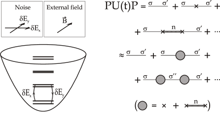
Figure 1: Left: Single electron lateral quantum dot in a magnetic field, which lifts the ground state degeneracy. Virtual transitions to excited states are induced by weak fluctuations of the external fields $\delta E_{x}(t)$, $\delta E_{y}(t)$. Right: Graphical representation of the evolution operator. Virtual transitions to excited states $n$ (wavy lines) are integrated out to yield an effective Hamiltonian within the doublet subspace.

In case of time-reversal symmetry the ground state of the dot is two-fold degenerate. This degeneracy is split in an external magnetic field. If $g\mu_{B}B\ll\omega_{0}$, and as long as the noise is adiabatic with respect to the orbital level splitting, $T\ll\omega_{0}$, the dynamics of the spin remains constrained to these two states. Under these conditions (following the method described in Ref. Hutter et al., ) we can derive an effective Hamiltonian for the two lowest eigenstates $|\sigma=\pm\rangle$ by expanding the evolution operator $U(t)=\mathrm{T\;exp}\{-i\int_{0}^{t}dt^{\prime}\;{\delta V}_{\rm int}(t^{\prime})\}$ and projecting to the subspace $\{|\sigma\rangle\}$ as sketched in Fig. 1. This yields

$$PU(t)P=1-i\int_{0}^{t}dt_{1}P\delta V_{\rm int}(t_{1})P$$

$$-\int\int_{t_{1}>t_{2}}P\delta V_{\rm int}(t_{1})P\delta V_{\rm int}(t_{2})P$$ (4)

$$-\int\int_{t_{1}>t_{2}}P\delta V_{\rm int}(t_{1})(1-P)\delta V_{\rm int}(t_{2})P+\ldots\;.$$

Here $\delta V_{\rm int}(t)$ denotes the fluctuating part of the Hamiltonian in the interaction representation and $P=\sum_{\sigma}|\sigma\rangle\langle\sigma|$. We separated terms that involve direct transitions between the two lowest states from transitions via excited states. In the spirit of an adiabatic approximation, these latter processes can be integrated out to yield an effective Hamiltonian in the two-dimensional subspace. Technically, this is performed by introducing slow and fast variables, $t\equiv(t_{1}+t_{2})/2$ and $\tau\equiv t_{1}-t_{2}$, in the last term of Eq. (4),

$$\sim\;e^{-it(\epsilon_{\sigma}-\epsilon_{\sigma^{\prime}})-i\tau\left[\frac{1}{2}(\epsilon_{\sigma}+\epsilon_{\sigma^{\prime}})-\epsilon_{n}\right]}\;\delta V_{\sigma n}(t_{1})\delta V_{n\sigma^{\prime}}(t_{2})\;,$$

expanding the interaction potential in $\tau$ as $\delta V(t_{1,2})\approx\delta V(t)\pm\frac{\tau}{2}\;\frac{d}{dt}{\delta V}(t)+\dots$, and integrating with respect to $\tau$. Here $\epsilon_{\sigma}$ and $\epsilon_{n}$ denote the eigenenergies of the lowest doublet and higher eigenstates of $H_{0}$, respectively. In this way the last term in Eq. (4) becomes local in time. Retaining only processes up to 2nd order, we find an effective Hamiltonian within the lowest-energy two-dimensional subspace, characterized by the ’pseudospin’ Pauli matrices $\tau_{x,y,z}$,

$$H_{\mathrm{eff}} = -\frac{1}{2}B_{\rm eff}\;{\tau_{z}}+X^{\mu}\vec{C}^{(1)}_{\mu}\cdot\vec{\tau}+X^{\mu}X^{\nu}\vec{C}^{(2)}_{\mu\nu}\cdot\vec{\tau}$$ (5)

$$+ \frac{1}{2}\left(\dot{X}^{\mu}X^{\nu}-X^{\mu}\dot{X}^{\nu}\right)\vec{C}^{(3)}_{\mu\nu}\cdot\vec{\tau}\;.$$

Due to the spin-orbit coupling, which is not assumed to be weak, eigenstates do not factorize into orbital and spin sectors (hence the term ’pseudospin’). The static effective field, ${\vec{B}}_{\rm eff}\equiv(\epsilon_{+}-\epsilon_{-})\hat{z}$, accounts for the spin-orbit renormalization of the $g$-factor and defines the $\hat{z}$ direction in the doublet space. The couplings $\vec{C}^{(i)}$, determining the effective fluctuating magnetic fields felt by the pseudospin, are given by

$$\left[\vec{C}^{(1)}_{\mu}\cdot\vec{\tau}\right]_{\sigma,\sigma^{\prime}}=\hat{O}^{\mu}_{\sigma\sigma^{\prime}}\ ,$$ (6)

$$\left[\vec{C}^{(2)}_{\mu\nu}\cdot\vec{\tau}\right]_{\sigma,\sigma^{\prime}}=-{\sum_{n}}^{\prime}\frac{\hat{O}^{\mu}_{\sigma n}\hat{O}^{\nu}_{n\sigma^{\prime}}}{\frac{\epsilon_{\sigma}+\epsilon_{\sigma^{\prime}}}{2}-\epsilon_{n}}\ ,$$ (7)

$$\left[\vec{C}^{(3)}_{\mu\nu}\cdot\vec{\tau}\right]_{\sigma,\sigma^{\prime}}=-i\,{\sum_{n}}^{\prime}\frac{\hat{O}^{\mu}_{\sigma n}\hat{O}^{\nu}_{n\sigma^{\prime}}}{\left(\frac{\epsilon_{\sigma}+\epsilon_{\sigma^{\prime}}}{2}-\epsilon_{n}\right)^{2}}\ .$$ (8)

The summation is restricted to excited states of higher doublets $n\neq\sigma,\sigma^{\prime}$. We do not provide explicit expressions for the eigenenergies $\epsilon_{\sigma}$, $\epsilon_{n}$, matrix elements $\hat{O}^{\mu}_{\sigma\sigma^{\prime}}$, $\hat{O}^{\mu}_{\sigma n}$, or couplings $\vec{C}^{(i)}$, but below we will evaluate them numerically and provide quantitative estimates for a generic model. We further note that both $\vec{C}^{(1)}_{\mu}$ and $\vec{C}^{(3)}_{\mu\nu}$ turn out to be transversal to ${\vec{B}}_{\rm eff}$, therefore contributing only to relaxation, whereas $\vec{C}^{(2)}_{\mu\nu}$ has in general also a parallel component that leads to pure dephasing.

In time-reversal symmetric situation, (i.e. for $B=0$), the first three terms of Eq. (5) vanish identically Khaetskii and Nazarov (2001). Only the last term survives, and leads to spin dephasing. It has a geometrical origin. To demonstrate this, let us assume that the fluctuating (adiabatic) fields $X_{\mu}$ are classical. We introduce the instantaneous ground states of the Hamiltonian, $|\Phi_{n}(t)\rangle\equiv|\Phi_{n}(X_{\mu}(t))\rangle$ defined through the equation

$$[H_{0}+\delta V(X_{\mu})]|\Phi_{n}(X_{\mu})\rangle=E_{n}(X_{\mu})|\Phi_{n}(X_{\mu})\rangle\;.$$ (9)

Noting that, to lowest order perturbation theory, the two degenerate instantaneous ground states are simply given by $|\Phi_{\sigma}(X_{\mu})\rangle\approx|\sigma\rangle+{\sum_{n}}^{\prime}|n\rangle{\langle n|\delta V|\sigma\rangle}/({\epsilon_{\sigma}-\epsilon_{n}})\;,$ we can rewrite the last term in Eq. (5) in the familiar form

$$H^{\mathrm{eff}}_{\sigma\sigma^{\prime}}(B=0)=-i\langle{\frac{d\Phi_{\sigma}}{dt}|\Phi_{\sigma^{\prime}}}\rangle\;,$$ (10)

which shows clearly that the last term is due to a generalized (possibly non-Abelian) Berry phase Berry (1984); Wilczek and Zee (1984); Mead (1987) acquired in a degenerate 2D subspace. In vanishing magnetic field, Eq. (10) can be shown to hold to all orders of perturbation theory within the adiabatic approximation. If at least two linearly independent fluctuating fields couple to the dot, they can produce a random Berry phase for the system and cause geometric dephasing at $B=0$. When more noise components are present, the Berry phase may become non-Abelian and all components of the spin may decay.

So far, our treatment has been rather general, applicable for arbitrary noise properties and dot geometries. In its full glory, Eq. (5) describes the motion of the pseudo-spin coupled to three fluctuating “magnetic fields”. In general, the dynamics induced by these non-commuting fields is complicated. To obtain a qualitative understanding of the dynamics we analyze the spin relaxation and pure dephasing times Bloch (1957), $T_{1}$ and $T_{2}^{*}$ (with $1/T_{2}=1/2T_{1}+1/T_{2}^{*}$). They are defined only for sufficiently strong effective fields, $B_{\rm eff}\gg 1/T_{1},\;1/T^{*}_{2}$. In the limit $B=0$ we evaluate what we call the geometrical dephasing time $T_{\rm geom}$. For the quantitative estimate we consider a parabolic confining potential, $V({\bf r})=\frac{m^{*}\omega_{0}^{2}}{2}|{\bf r}|^{2}$ with level spacing $\omega_{0}$ and typical size $x_{0}=1/\sqrt{\omega_{0}m^{*}}$. Furthermore, we take into account only dipolar fluctuations, $\hat{X}\equiv e\delta E_{x}x_{0}$ and $\hat{Y}\equiv e\delta E_{y}x_{0}$ coupling to the operators ${\hat{O}}_{X}\equiv x/x_{0}$ and ${\hat{O}}_{Y}\equiv y/x_{0}$, respectively. We assume the two components $\hat{X}$ and $\hat{Y}$ to be independent of each other, but with identical noise spectra, $S_{X}(\omega)=S_{Y}(\omega)=S(\omega)=\pi\varrho(\omega){\rm coth}(\omega/2T)$, with $\varrho(\omega)$ being the spectral function of the bosonic environment (phonons or photons).

The spectral function $\varrho(\omega)$ for phonons can be estimated along the lines of Ref. Khaetskii and Nazarov, 2001. For the parameters specified in Ref. Golovach et al., 2004 we find for piezoelectric phonons in typical GaAs heterostructures at low frequencies, $\varrho_{\rm ph}(\omega)=x_{0}^{2}\;\lambda_{\rm ph}\;\omega^{3}$ with $\lambda_{\rm ph}\approx 4\cdot 10^{-6}{\rm K}^{-2}{\rm nm}^{-2}$ foo (a). With these parameters we obtain relaxation rates generated by the first term in Eq. (5) that coincide with those of Ref. Golovach et al., 2004 at not too high values of the field foo (b). Similar values are obtained for the parameters of Ref. Stano and Fabian, . For Ohmic fluctuations the spectral function is linear at low frequencies, $\varrho_{\Omega}(\omega)=\lambda_{\Omega}\;\omega$ Leggett et al. (1987); Weiss (1999). The prefactor $\lambda_{\Omega}$ depends on the dimensionless impedance of the circuit, $\lambda_{\Omega}\sim\frac{e^{2}}{h}\;{\rm Re}[Z]$. For typical values of the sheet resistance of the 2-DEG ($10^{2}-10^{3}\Omega/\Box$) we estimate it to be in the range $0.1>\lambda_{\Omega}>0.01$. For $1/f$ noise the power spectrum is $S(\omega)=\lambda_{1/f}/|\omega|$. We will further comment on its strength below.

We first estimate the contributions $T_{1}^{(i)}$ and $T_{2}^{*(i)}$, derived from the three terms ($i=1,2,3$) in Eq. (5), for a non-vanishing in-plane magnetic field, $B_{\rm eff}\gg 1/T_{1},\;1/T^{*}_{2}$. The coupling ${\vec{C}}^{(1)}$ turns out to be perpendicular to ${\vec{B}}_{\rm eff}$ Golovach et al. (2004), and for low magnetic fields and weak spin-orbit coupling is proportional to $|{\vec{C}}^{(1)}|\sim\frac{B}{x_{0}\omega_{0}^{2}}\;\max\{{\alpha},{\beta}\}$. This fluctuating field therefore contributes to the $T_{1}$-relaxation only,

$$\frac{1}{T_{1}^{(1)}}=2\left(|\vec{C}^{(1)}_{X}|^{2}+|\vec{C}^{(1)}_{Y}|^{2}\right)\;S_{X}(B_{\rm eff})\ .$$ (11)

It scales as $1/T_{1}^{(1)}\sim B^{2}\max\{B,T\}$ for Ohmic dissipation and as $\sim B^{4}\max\{B,T\}$ for phonons. As a consequence, for dots with level spacing in the range $\omega_{0}\approx 1\dots 10\;{\rm K}$ Ohmic fluctuations dominate over phonons for low fields with $B<1\dots 3\;{\rm T}$.

The second term, $|{\vec{C}}^{(2)}|\sim\frac{B}{x_{0}^{2}\omega_{0}^{4}}\max\{\alpha^{2},\beta^{2}\}$ gives rise to both relaxation and dephasing. The two rates are

$$\frac{1}{T_{1}^{(2)}}=4\left(|\vec{C}^{(2,\perp)}_{XX,s}|^{2}+|\vec{C}^{(2,\perp)}_{YY,s}|^{2}+2|\vec{C}^{(2,\perp)}_{XY,s}|^{2}\right)S_{XY}(B_{\rm eff})\;,$$

$$\frac{1}{T_{2}^{*(2)}}=4\left(|\vec{C}^{(2,\parallel)}_{XX,s}|^{2}+|\vec{C}^{(2,\parallel)}_{YY,s}|^{2}+2|\vec{C}^{(2,\parallel)}_{XY,s}|^{2}\right)S_{XY}(0)\;,$$

$$S_{XY}(\omega)=\frac{\pi}{2}\int d\tilde{\omega}\;\frac{\varrho(\frac{\omega+\tilde{\omega}}{2})\varrho(\frac{\omega-\tilde{\omega}}{2})}{1-\cosh(\tilde{\omega}/2T)/\cosh(\omega/2T)}\ ,$$

with $\vec{C}^{(2,\perp/\parallel)}_{\mu\nu,s}$ denoting the symmetrized component of ${\vec{C}}^{(2)}_{\mu\nu}$ perpendicular/parallel to ${\vec{B}}_{\rm eff}$. Thus, for Ohmic dissipation ${1}/{T_{1}^{(2)}}$ vanishes as $\sim B^{2}\max\{B^{3},T^{3}\}$, while for phonons it scales as $\sim B^{2}\max\{B^{7},T^{7}\}$.

$\vec{C}^{(3)}$ is also perpendicular to ${\vec{B}}_{\rm eff}$. Its contribution to the relaxation is

$$\frac{1}{T_{1}^{(3)}} = 2|\vec{C}^{(3)}_{XY,a}|^{2}S_{\dot{X}Y-X\dot{Y}}(B_{\rm eff})\;,$$ (12)

$$S_{\dot{X}Y-X\dot{Y}}(\omega) = \frac{\pi}{2}\int d\tilde{\omega}\;\frac{\tilde{\omega}^{2}\varrho(\frac{\omega+\tilde{\omega}}{2})\varrho(\frac{\omega-\tilde{\omega}}{2})}{1-\cosh(\tilde{\omega}/2T)/\cosh(\omega/2T)}\;,$$

with $\vec{C}^{(3)}_{\mu\nu,a}$ being the anti-symmetrized component of ${\vec{C}}^{(3)}_{\mu\nu}$. Most importantly, with $|{\vec{C}}^{(3)}_{XY}|\sim\frac{1}{x_{0}^{2}\omega_{0}^{4}}\max\{\alpha^{2},\beta^{2}\}$, the rate ${1}/{T_{1}^{(3)}}$ approaches a non-zero value at low fields, $1/T_{1},1/T_{2}^{*}\ll B\ll T$, and scales as $\sim\max\{B^{5},T^{5}\}$ for Ohmic dissipation and $\sim\max\{B^{9},T^{9}\}$ for phonons.

Finally, at $B=0$ the geometric dephasing rate is given by ${1}/{T_{1}^{(3)}}$, extrapolated to zero field

$$\frac{1}{T_{\rm geom}}=2|\vec{C}^{(3)}_{XY,a}|^{2}S_{\dot{X}Y-X\dot{Y}}(\omega\sim 0)\ .$$ (13)

In our example with only two noise components this process dephases only the components of the spin perpendicular to $\vec{C}^{(3)}_{XY}$.

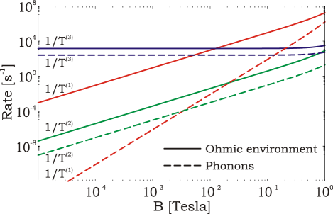
Figure 2: Spin relaxation rates for a GaAs quantum dot with level spacing $\omega_{0}=1{\rm K}$ as function of the Zeeman field. We chose a temperature $T=100\;{\rm mK}$ and Ohmic coupling $\lambda_{\Omega}=0.05$. Below $B^{*}\approx 1\;{\rm T}$ spin relaxation is dominated by coupling to Ohmic fluctuations. For $B<B^{**}\approx 15\;{\rm mT}$ geometrical spin relaxation due to coupling to Ohmic fluctuations dominates. For all $B$ values plotted, the Bloch-Redfield consistency requirement, $B_{\mathrm{eff}}\gg 1/T^{(i)}$, is satisfied.

The relaxation rates corresponding to the different terms in Eq. (5) and various noise sources are shown in Fig. 2. Clearly, for external fields $B<B^{*}\approx 1\dots 3\;{\rm T}$ Ohmic fluctuations provide the leading relaxation mechanism. The crossover field $B^{*}$ is not very sensitive to the specific value of the spectral parameter $\lambda_{\Omega}$ and is independent of the spin-orbit coupling. Below a second crossover field, $B^{**}\approx 15{\rm mT}$, the geometric dephasing induced by Ohmic fluctuations starts to dominate. This second crossover scale is very sensitive to the spin-orbit coupling and temperature, scaling as $B^{**}\sim\max\{\alpha,\beta\}(1/x_{0})(T/\omega_{0})^{2}$. E.g. for a level spacing $\omega_{0}\sim 1{\rm K}$ and temperature $T=100\;{\rm mK}$ ($T=50\;{\rm mK}$) the Berry phase mechanism gives a relaxation time of the order of $700\;{\rm\mu s}$ ($20\;{\rm ms}$). For even lower temperatures or smaller dots with level spacing $\omega_{0}\sim 10{\rm K}$ the $B\to 0$ relaxation time is quickly pushed up to the range of seconds.

Finally, we comment on the effect of $1/f$ noise. In most cases, the non-symmetrized correlators for $1/f$ noise, needed to calculate correlators as $S_{XY}$ or $S_{XX}$, are not known. Yet, for $|\omega|\ll T$ we can provide an estimate $S_{XY}(\omega)\approx\int\limits_{-T}^{T}\frac{d\tilde{\omega}}{2\pi}S_{X}(\omega-\tilde{\omega})S_{Y}(\tilde{\omega})$, and similarly for $S_{\dot{X}Y-X\dot{Y}}$. The $B=0$ geometrical dephasing rate due to the $1/f$ noise can be estimated as $T_{\rm geom}^{-1}\approx|{\vec{C}}^{(3)}_{XY}|^{2}\lambda_{1/f}^{2}(T)\,\omega_{c}$, where $\omega_{c}$ is the upper frequency cut-off for the $1/f$ noise Ithier et al. (2005). Accounting for the high-frequency (Ohmic) noise, sometimes observed to be associated with the $1/f$ noise Astafiev et al. (2004); Shnirman et al. (2005); Faoro et al. (2005); Astafiev et al. (2006), the estimate becomes $T_{\rm geom}^{-1}\approx|{\vec{C}}^{(3)}_{XY}|^{2}\lambda_{1/f}^{2}(T)\,T$. While the $1/f$ noise of background charge fluctuations is well studied in mesoscopic systems, the amplitude of the $1/f$ noise of the electric field in quantum dot systems is yet to be determined. If we assume that this noise is due to two-level systems at the interfaces of the top gate electrodes, we conclude that in the parameter range explored here, the effect of $1/f$ noise is less important than that of Ohmic fluctuations. However, in quantum dots with large level spacings in the low-temperature and low-field regime, these fluctuations could dominate over the effect of Ohmic fluctuations and eventually determine the spin relaxation time.

We thank J. Fabian for valuable discussions. This work has been supported through a research network of the Landesstiftung Baden-Württemberg gGmbH, by Hungarian Grants OTKA Nos. NF061726, T046267, and T046303, and the SQUBIT2 project IST-2001-39083.

References

- Elzerman et al. (2004) J. M. Elzerman et al., Nature 430, 431 (2004).
- Petta et al. (2005) J. R. Petta et al., Science 309, 2180 (2005).
- Loss and DiVincenzo (1998) D. Loss and D. P. DiVincenzo, Phys. Rev. A 57, 120 (1998).
- Khaetskii et al. (2002) A. V. Khaetskii, D. Loss, and L. Glazman, Phys. Rev. Lett. 88, 186802 (2002).
- Khaetskii and Nazarov (2001) A. V. Khaetskii and Y. V. Nazarov, Phys. Rev. B 64, 125316 (2001).
- Woods et al. (2002) L. M. Woods, T. L. Reinecke, and Y. Lyanda-Geller, Phys. Rev. B 66, 161318 (2002).
- Golovach et al. (2004) V. N. Golovach, A. Khaetskii, and D. Loss, Phys. Rev. Lett. 93, 016601 (2004).
- Aronov and Lyanda-Geller (1993) A. G. Aronov and Y. B. Lyanda-Geller, Phys. Rev. Lett. 70, 343 (1993).
- Whitney et al. (2005) R. S. Whitney, Y. Makhlin, A. Shnirman, and Y. Gefen, Phys. Rev. Lett. 94, 070407 (2005).
- Elliott (1954) R. J. Elliott, Phys. Rev. 96, 266 (1954).
- Serebrennikov (2004) Y. A. Serebrennikov, Phys. Rev. Lett. 93, 266601 (2004).
- Abrahams (1957) E. Abrahams, Phys. Rev. 107, 491 (1957).
- (13) M. Borhani, V. N. Golovach, and D. Loss, cond-mat/0510758.
- foo (a) For GaAs , , longitudinal and transverse sound velocities , , piezoelectric const. , density , . For the quantitative analysis we considered Dresselhaus coupling with .
- Winkler (2003) R. Winkler, Spin-orbit coupling effects in two-dimensional electron and hole systems, Springer Tracts in Modern Physics (2003).
- (16) C. Hutter, A. Shnirman, Y. Makhlin, and G. Schön, cond-mat/0602086, accepted in Europhys. Lett.
- Berry (1984) M. V. Berry, Proc. R. Soc. London A 392, 45 (1984).
- Wilczek and Zee (1984) F. Wilczek and A. Zee, Phys. Rev. Lett. 52, 2111 (1984).
- Mead (1987) C. A. Mead, Phys. Rev. Lett. 59, 161 (1987).
- Bloch (1957) F. Bloch, Phys. Rev. 105, 1206 (1957).
- foo (b) For larger frequencies the approximation is not valid since the wavelength of relevant phonons becomes comparable to the size of the dot.
- (22) P. Stano and J. Fabian, cond-mat/0512713.
- Leggett et al. (1987) A. J. Leggett et al., Rev. Mod. Phys. 59, 1 (1987).
- Weiss (1999) U. Weiss, Quantum dissipative systems (World Scientific, Singapore, 1999), 2nd ed.
- Ithier et al. (2005) G. Ithier et al., Phys. Rev. B 72, 134519 (2005).
- Astafiev et al. (2004) O. Astafiev, Y. A. Pashkin, Y. Nakamura, T. Yamamoto, and J. S. Tsai, Phys. Rev. Lett. 93, 267007 (2004).
- Shnirman et al. (2005) A. Shnirman, G. Schön, I. Martin, and Y. Makhlin, Phys. Rev. Lett. 94, 127002 (2005).
- Faoro et al. (2005) L. Faoro, J. Bergli, B. L. Altshuler, and Y. M. Galperin, Phys. Rev. Lett. 95, 046805 (2005).
- Astafiev et al. (2006) O. Astafiev, Y. A. Pashkin, Y. Nakamura, T. Yamamoto, and J. S. Tsai, Phys. Rev. Lett. 96, 137001 (2006).