Magnetic Excitations of Stripes and Checkerboards in the Cuprates

Abstract

We discuss the magnetic excitations of well-ordered stripe and checkerboard phases, including the high energy magnetic excitations of recent interest and possible connections to the “resonance peak” in cuprate superconductors. Using a suitably parametrized Heisenberg model and spin wave theory, we study a variety of magnetically ordered configurations, including vertical and diagonal site- and bond-centered stripes and simple checkerboards. We calculate the expected neutron scattering intensities as a function of energy and momentum. At zero frequency, the satellite peaks of even square-wave stripes are suppressed by as much as a factor of $34$ below the intensity of the main incommensurate peaks. We further find that at low energy, spin wave cones may not always be resolvable experimentally. Rather, the intensity as a function of position around the cone depends strongly on the coupling across the stripe domain walls. At intermediate energy, we find a saddlepoint at $(\pi,\pi)$ for a range of couplings, and discuss its possible connection to the “resonance peak” observed in neutron scattering experiments on cuprate superconductors. At high energy, various structures are possible as a function of coupling strength and configuration, including a high energy square-shaped continuum originally attributed to the quantum excitations of spin ladders. On the other hand, we find that simple checkerboard patterns are inconsistent with experimental results from neutron scattering.

I Introduction

Strong correlations in electronic systems, and especially competing interactions, can cause mesoscale electronic structure to spontaneously develop. In cuprate superconductors and the related nickelate compounds, several locally inhomogenous electronic phases have been proposed, involving charge order, spin order, or both. Several experimental probes corroborate some level of local order, including STM,checknccoc ; hoffman ; aharon neturon scattering,mookchg ; tranquada04a ; hayden04 ; aeppli , NMRhammelwipeout and $\mu$SR studies.neidermeyer Recent experimental advances have made possible the detection of high energy neutron scattering spectra.hayden04 ; tranquada04a ; buyers04 There has been much interest in the interpretation of these spectra in the cuprates, especially since the high energy results from neutron scattering on La_2-xBa_xCuO₄ (LBCO) and YBa₂Cu₃O_6+δ (YBCO) exhibit universal behavior.tranquada04a ; hayden04 This paper extends the previous work of Refs.spinprb1 ; spinprl to look at a broader range of ordered structures, and also to explore the scattering patterns which are possible at high energies. It has been suggested, for example, that the high energy magnetic excitations in LBCO and YBCO may be due to the quantum excitations of stripes.vojta-ulbricht ; uhrig04a ; tranquada04a ; seibold04 We have reported elsewherespinprl that high energy excitations near a quantum critical point (QCP) to disordered laddersvojta-ulbricht ; uhrig04a ; seibold04 ; vojta-sachdev can strongly resemble semiclassical excitations, due to the small critical exponent $\eta=0.037$ associated with this QCP.

One continuing mystery about the low energy results has been the lack of observed spin satellite peaks in neutron scattering, and also that spin wave cones are rarely observed in the cuprates. Rather, what is often seen in the low energy regime may be more accurately termed “legs of scattering”. Both of these results have raised questions about a “stripe” interpretation of the data. We show below that at $\omega=0$, satellite peaks for even the most extreme case of square-wave spin stripes have very low intensity, and may not be resolvable without very high experimental resolution. In addition, although a spin ordered state results in spin wave cones due to Goldstone’s theorem, the intensity is not always uniform. Rather, the intensity can be gathered on the inner branch of the spin wave cones [the side nearest $(\pi,\pi)$], or on the outer branch, depending upon the relative strength of the spin coupling across the charge stripes. For this reason, while spin wave cones are always present for ordered spin stripes, they may not yet be resolvable experimentally.

An important point we wish to emphasize is that although stripes are a unidirectional modulation in an otherwise antiferromagnetic texture, they are a fully two-dimensional (2D) spin order, with a 2D magnetic Bravais lattice, which gives rise to 2D scattering signals at all energies. Our results never show streaks of scattering in the low energy structure, although streaks are possible in the high energy structure for weak coupling, as we report below.

II Model and Method

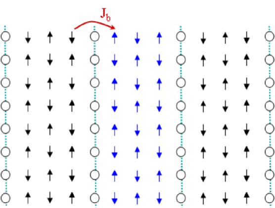
(a) VS4

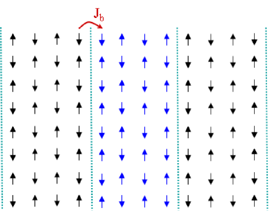
(b) VB4

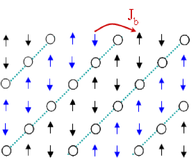
(c) DS3

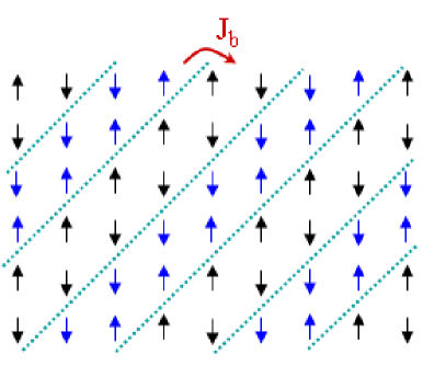
(d) DB2

Figure 1: (Color online) Stripe configurations studied in this paper. The coupling between nearest neighbor spins is $J_{a}$, and the coupling between spins across a domain wall is $J_{b}$, as indicated in the figures. (a) VS4: Vertical site-centered stripes with spacing $d=4$. (b) VB4: Vertical bond-centered stripes with spacing $d=4$. (c) DS3: Diagonal site-centered stripes with spacing $d=3$. (d) DB2: Diagonal bond-centered stripes with spacing $d=2$.

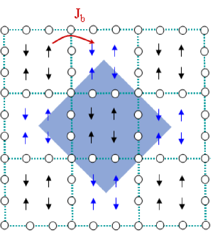
(a) CS3

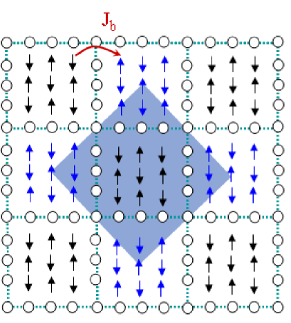
(b) CS4

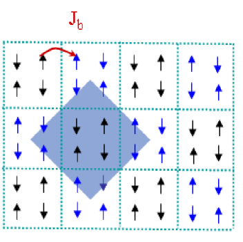
(c) CB2

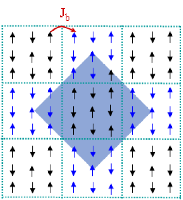
(d) CB3

Figure 2: (Color online) Checkerboard patterns. The coupling between nearest neighbor spins is $J_{a}$, and the coupling between spins across a domain wall is $J_{b}$, as indicated in the figures. (a) CS3: Checkerboard sited-centered pattern with spacing $d=3$. (b) CS4: Checkerboard site-centered pattern with spacing $d=4$. (c) CB2: Checkerboard bond-centered pattern with spacing $d=2$. (d)CB3: Checkerboard bond-centered pattern with spacing $d=3$.

In this work we concentrate on static stripes and checkerboards as arrays of antiphase domain walls in an otherwise antiferromagnetic texture. We are interested solely in the response of the spin degrees of freedom. The dynamics of the charge component which must reside on every domain wall is to renormalize the effective spin couplings in the Hamiltonian. We thus use a suitably parametrized Heisenberg model to describe the elementary excitations of spin stripes, employing a modulation of the exchange integral to capture the effective spin coupling in a well ordered stripe or checkerboard phase.

$$H=\frac{1}{2}\sum_{\mathbf{r},\mathbf{r^{\prime}}}J_{\mathbf{r},\mathbf{r^{\prime}}}\mathbf{S}_{\mathbf{r}}\mathbf{S}_{\mathbf{r^{\prime}}},$$ (1)

where $J_{\mathbf{r},\mathbf{r^{\prime}}}$ is the effective spin coupling. We work in units where $\hbar=1$. Nearest neighbor couplings are antiferromagnetic with $J_{\mathbf{r},\mathbf{r^{\prime}}}=J_{a}>0$ within each antiferromagnetic patch. Couplings across a domain wall are different, and depend upon the configuration (such as spacing and direction of the domain walls). These are enumerated below. When comparing to, e.g., the cuprates (nickelates), our lattice corresponds to the copper (nickel) sites within the copper-oxygen (nickel-oxygen) planes. With these materials in mind, we restrict ourselves to patterns embedded in a two-dimensional square lattice.

II.1 Stripe and Checkerboard Configurations

In the presence of a host crystal, stripes are constrained by the symmetry of the crystal to run along major crystallographic directions. We consider two classes of stripe patterns, vertical and diagonal, as well as checkerboard patterns. These classifications concern the pattern of the antiphase domain walls in the antiferromagnetism. We use the term “vertical” to describe stripes whose domain walls run parallel to the Cu-O (Ni-O) bond direction, and the term “diagonal” to describe stripes that run $45^{o}$ from that direction. These stripe patterns are depicted in Fig. 1.

A further distinction between types of stripes and checkerboards depends on where the antiphase domain walls sit with respect to the atomic lattice. “Site-centered” stripes have domain walls which are centered on the sites of the square lattice (i.e. on the nickel or copper sites). These have antiferromagnetic coupling $J_{\mathbf{r},\mathbf{r^{\prime}}}=J_{b}>0$ across the domain wall. On the other hand, when the domain wall is situated between two square lattice sites (i.e. between nickel or copper sites, on the planar oxygens), the stripes are “bond-centered”. In this case the coupling across the domain wall is effectively ferromagnetic (to preserve the antiphase nature of the domain walls), and $J_{b}<0$.sitecentered

Checkerboard patterns have been proposed to explain the real space structure observed in STM experiments on Bi₂Sr₂CaCu₂O_8+δhoffman (BSCCO) and Ca_2-xNa_xCuO₂Cl₂checknccoc (Na-CCOC). It is important to note that STM is a surface probe, and to date, the $4\times 4$ pattern observed in BSCCO and Na-CCOC has not been confirmed by neutron scattering or other bulk probes in these materials. Likewise, the $4\times 4$ pattern has not yet been confirmed via STM to be present in the lanthanum and yttrium compounds. Nevertheless, it has been noted that the length scale of the charge periodicity observed in BSCCO and Na-CCOC via STM is half that of the spin periodicity found in neutron scattering in related lanthanum-based and yttrium-based cuprate superconductors, and that therefore the two probes may be observing similar charge and spin modulations. Since the neutron scattering shows satellite peaks around antiferromagnetism, rather than a peak at the antiferromagnetic wavevector $(\pi,\pi)$, any universal spin texture which is consistent with the proposed checkerboard pattern must also incorporate antiphase domain walls in the corresponding spin texture. Representative, simple spin checkerboard configurations are shown in Fig. 2. The parameter $d$ is the spacing between domain walls. The low energy peaks of these simple checkerboard patterns are inconsistent with neutron scattering data,vojta-sachdev ; andersen03 as we will show in Sec. V, although more complicated checkerboard patternsabbamonte may be consistent.

We use the notation VSd,VBd,DSd and DBd to refer to vertical (V) or diagonal (D) stripes of spacing d in a site (S)- or bond (B)-centered configuration,spinprb1 as illustrated in Fig. 1. The notation CSd and CBd refers to checkerboards of site (S)- or bond (B)-centered domain walls which are $d$ lattice sites apart.

II.2 Spin-wave method

We use linear spin-wave theory to explore the semiclassical spinwave excitations of well-ordered spin stripes, as modeled by Eq. 1. Ladder operators may be used to rewrite the Hamiltonian in term of spin wave excitations above the semiclassical ground state:

$$H=\frac{1}{2}\sum_{<\mathbf{r},\mathbf{r^{\prime}}>}J_{\mathbf{r},\mathbf{r^{\prime}}}[S^{z}_{\mathbf{r}}S^{z}_{\mathbf{r^{\prime}}}+\frac{1}{2}(S^{+}_{\mathbf{r}}S^{-}_{\mathbf{r^{\prime}}}+S^{-}_{\mathbf{r}}S^{+}_{\mathbf{r^{\prime}}})].$$ (2)

The spin ladder operators may be approximated as Holstein-Primakoff bosons, a standard procedure described elsewhere,spinprb1 ; assa ; kruger03 in order to calculate the spin wave excitation spectrum as well as the zero-temperature dynamical structure factor,

$$S(\mathbf{k},\omega)=\sum_{f}\sum_{i=x,y,z}|\left<f|S^{i}(\mathbf{k})|0\right>|^{2}\delta(\omega-\omega_{f})$$ (3)

which is proportional to the expected neutron scattering intensity for single magnon excitations. Here $\left|0\right>$ is the magnon vacuum state and $\left|f\right>$ denotes the final state of the spin system with excitation energy $\omega_{f}$. We report single magnon excitations, and neglect possible spin-wave interactions since they are higher order effects.

III Results: Spectra of Vertical Stripes

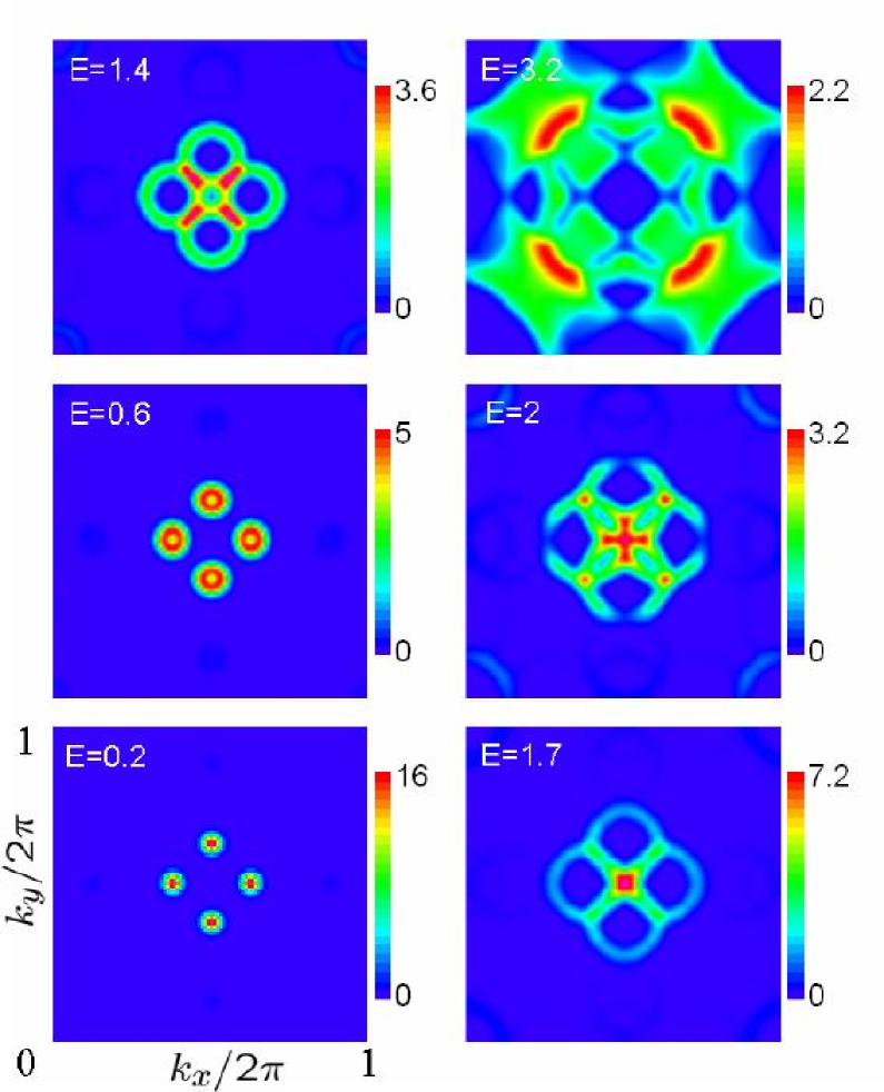
Figure 3: (Color online) VS4 at $J_{b}=0.4J_{a}$: Constant energy cuts with windows $0.2Ja$ for twinned vertical, site-centered stripes of spacing $d=4$ at $J_{b}=0.4J_{a}$. The energy $E$ is in units of $J_{a}S$.

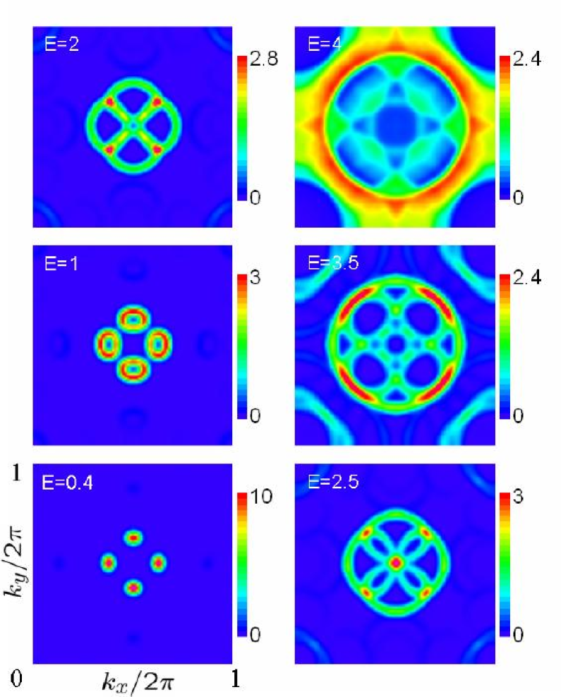
Figure 4: (Color online) VS4 at $J_{b}=J_{a}$: Constant energy cuts with windows $0.2Ja$ for twinned vertical, site-centered stripes of spacing $d=4$ at $J_{b}=J_{a}$. The energy $E$ is in units of $J_{a}S$.

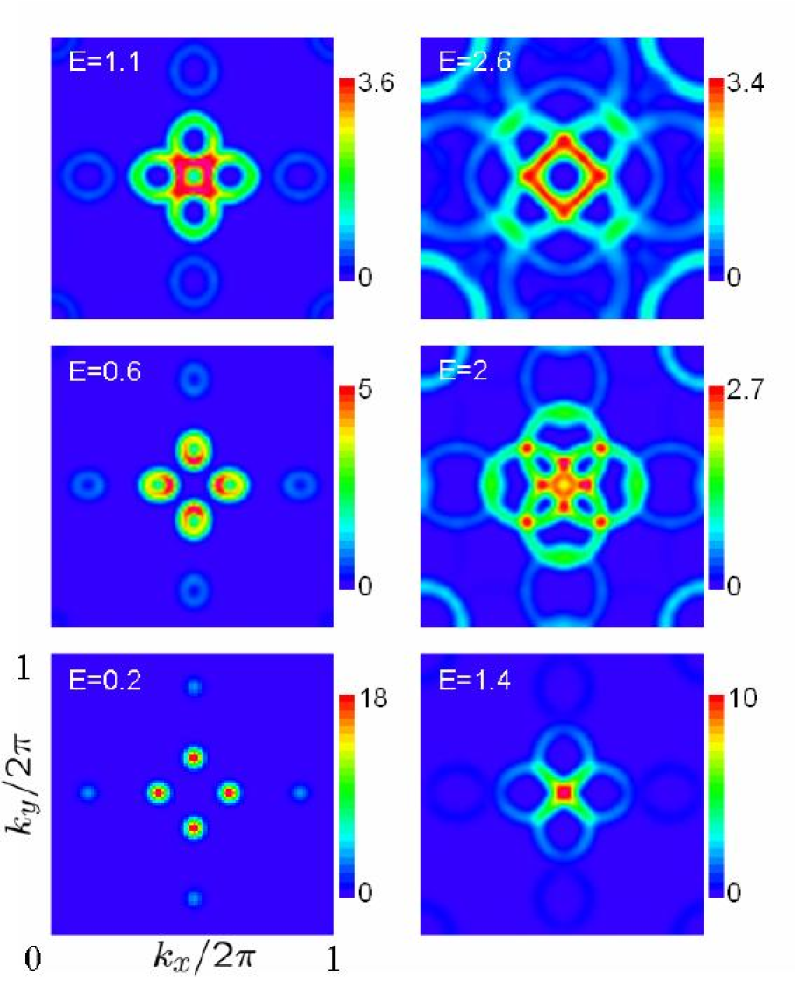
Figure 5: (Color online) VB4 at $J_{b}=-0.4J_{a}$: Constant energy cuts with windows $0.2Ja$ for twinned vertical, bond-centered stripes of spacing $d=4$ at $J_{b}=-0.4J_{a}$. The energy $E$ is in units of $J_{a}S$.

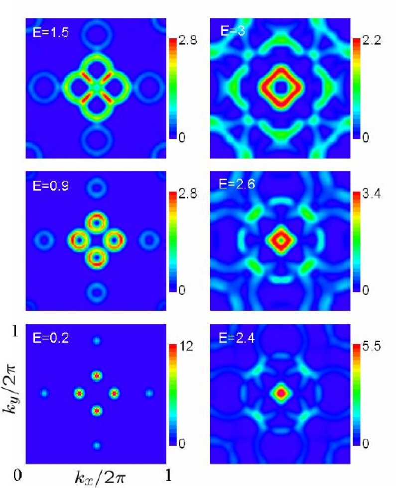
Figure 6: (Color online) VB4 at $J_{b}=-1.5J_{a}$: Constant energy cuts with windows $0.2Ja$ for twinned vertical, bond-centered stripes of spacing $d=4$ at $J_{b}=-1.5J_{a}$. The energy $E$ is in units of $J_{a}S$.

(a) VS4 Intensity Ratio

(b) VB4 Intensity Ratio

Figure 7: Intensity ratio between the “inner” and “outer” branches of the spin wave cones as a function of coupling ratio $|J_{b}/J_{a}|$ for vertical stripes. The ratio is calculated at constant low energy $E=0.4J_{a}S$. The solid points are our numerical calculations of the intensity ratio. The solid line is a fit to the results, as explained in the text. (a) VS4: Vertical, site-centered stripes of spacing $d=4$. (b) VB4: Vertical, bond-centered stripes of spacing $d=4$.

In this section, we report new results on the expected neutron scattering intensity at constant energy for vertical and diagonal stripes. In order to make a comparison with the experiments, we report constant energy plots of intensity in the $(k_{x},k_{y})$ plane. We work in tetragonal units, where the $k_{x}$ and $k_{y}$ directions are oriented along the Cu-O (Ni-O) bond direction and the antiferromagnetic wavevector is at $Q_{AF}=(\pi,\pi)$. In each plot, we integrate over an energy window of $\pm 0.2J_{a}S$. For vertical stripes, we show each plot for a twinned pattern of stripes, adding the intensity from domains rotated $90^{o}$ with respect to each other.

We first consider vertical stripes. Figs. 3 and 4 show results for vertical site-centered stripes at coupling ratio $J_{b}/J_{a}=0.4$ and $J_{b}/J_{a}=1.0$, respectively. Figs. 5 and 6 show results for vertical bond-centered stripes at coupling ratio $|J_{b}/J_{a}|=0.4$ and $|J_{b}/J_{a}|=1.5$, respectively.

The main incommensurate (IC) peaks indicating stripe order have high intensity at low energy in Figs. 3-6. However, the low energy satellite peaks are so weak as to be virtually unresolvable in the site-centered case (Figs. 3 and 4), while they are visible but still weak in the bond-centered case (Figs. 5 and 6). At $\omega=0$, the ratio between the main incommensurate peaks and the satellite peaks is $34$ for VS4, and it is $5.9$ for VB4. This is the maximum intensity ratio, for, e.g., a square wave pattern that follows Figs. 1 (a) and (b), in which every occupied site has the same spin moment. With such a dramatic suppression of the satellite peaks for VS4, and given the fact that the spin wave cone emanating from the satellite peaks in the site-centered case rapidly diminishes in intensity with increasing energy,spinprb1 it is not surprising that the satellite cones are too faint to be seen in the lowest energies of Figs. 3 and 4. Rather than evidence against stripes, the absence of observed satellite peaks may simply be due to insufficient experimental resolution, especially in the case of site-centered stripes. Any envelope softer than a square wave pattern will diminish the satellite peaks even further.wochner98a

At slightly higher energy (the middle left panel in Figs. 3-6), notice that the intensity on the spin wave cones can be different on the “inner branch,” the side closest to ($\pi,\pi$), and the “outer branch,” the side farthest from ($\pi,\pi$). In fact, in Fig. 5 (VB4 at $J_{b}/J_{a}=-0.4$), the intensity is strongest on the inner branch. On the other hand, at higher coupling ratios (Figs. 4 and 6), the strongest intensity is on the outer branch. The intensity ratio between inner and outer branches is a function of the coupling ratio $|J_{b}/J_{a}|$, as shown in Fig. 7. To obtain the figure, we have taken a cut through $k$-space perpendicular to the stripe direction, along $(k_{x},\pi)$, and restricted the plot to a low energy, $E=0.4J_{a}S$ . We divide the peak intensity at the inner branch of the spin wave cone by the peak intensity of the outer branch of the spin wave cone to derive the inner to outer branch intensity ratio in Fig. 7. Based on a fit of the results in Fig. 7, we find the following functional form for the intensity ratio of inner to outer branches for vertical stripes of spacing $d=4$:

$${S(\mathbf{k}_{\rm in},E_{o})\over S(\mathbf{k}_{\rm out},E_{o})}=a+{b\over{c+|J_{b}/J_{a}|^{\mu}}}~{},$$ (4)

where $\mathbf{k}_{\rm in}$ denotes the wavevector of the inner branch of the spin wave cone on the $(\pi,\pi)$ side, and $\mathbf{k}_{\rm out}$ denotes the wavevector of the outer branch away from $(\pi,\pi)$ at a particular energy $E_{o}$. For VS4 (site-centered stripes) at $E_{o}=0.4J_{a}S$ we find that $a=0.85$, $b=0.076$, $c=0$, and $\mu=0.89$. For VB4 (bond-centered stripes) at $E_{o}=0.4J_{a}S$ we find that $a=0.84$, $b=0.18$, $c=-0.033$, and $\mu=0.84$. For both site- and bond-centered stripes, for small enough $|J_{b}/J_{a}|$, the intensity ratio is so dramatic that without sufficiently high resolution, the entire spin wave cone will not be resolvable, and instead only “legs of scattering” will be visible. Several neutron scattering experiments on the cuprates report this kind of behavior,tranquada04a ; hayden04 ; mookchg and our calculations here indicate that the behavior is simply due to weak effective spin coupling across the charge stripes.

For a range of coupling ratios, the acoustic band has a saddlepoint at $(\pi,\pi)$ which has many similarities to the “resonance peak” observed in the cuprates. These saddlepoints can be seen in the bottom right panel of Figs. 3-6. Here, the intensity is gathered into one main peak at the antiferromagnetic wavevector $Q_{AF}$, where the maximum intensity is higher than that at nearby energies. The saddlepoint structure gives rise to an hourglass shape emanating from the resonance peak for twinned stripes in energy vs wavevector plots.uhrigsaddlepoint ; mookchg ; ybco6.7 ; ybco ; normanhourglass The resonance peak associated with a saddlepoint is more pronounced at low coupling ratio. For stronger coupling ratio, the weight in the spin wave cones is shifted to the outer branch, and the extra intensity due to the saddlepoint at ($\pi,\pi$) is reduced.

For the case of vertical, site-centered stripes of spacing $p=4$ (VS4), for $J_{b}=0.05J_{a}$, the resonance energy is $E_{\rm res}=0.63J_{a}S$, and for $J_{b}=0.2J_{a}$, the saddlepoint is at $E_{\rm res}=1.2J_{a}S$. Assuming the value of $J_{a}$ ($\approx 140{\rm meV}$coldea01 ) is relatively unchanged upon doping, this gives a range of $E_{\rm res}=44-84{\rm meV}$. This encompasses the range $E_{\rm res}=50-60{\rm meV}$ given in Ref. tranquada04a for the resonance peak in LBCO. For the case of vertical, bond-centered stripes of the same spacing (VB4), with $J_{b}=0.05J_{a}$, the saddlepoint is at $E_{\rm res}=0.6J_{a}S$, and for $J_{b}=0.2J_{a}$, $E_{\rm res}=1.1J_{a}S$. This corresponds to a range of $E_{\rm res}=42-77{\rm meV}$, again encompassing the experimental range $E_{\rm res}=50-60{\rm meV}$ in Ref. tranquada04a . This would indicate that to match the resonance energy in LBCO requires that $0.05J_{a}\lesssim J_{b}\lesssim 0.2J_{a}$.spinprl

Although doping is not explicitly in our model (rather we treat the stripe spacing in a phenomenological manner), low energy neutron scattering indicates that the stripes move closer together as doping is increased.yamada ; mook2 The energy of the saddlepoint resonance increases monotonically as the stripes are moved closer together in our model, holding $J_{a}$ and $J_{b}$ fixed. If $J_{a}$ and $J_{b}$ are relatively independent of doping (and we believe this is physically reasonable), then we would expect doping to increase the energy scale of, e.g., the resonance, as is observed in underdoped cuprates. However, predicting how $J_{a}$ and $J_{b}$ depend on doping is beyond the scope of our present model. Another important piece of physics in the cuprates is that the intensity of the“resonance peak” increases below $T_{c}$. However, since we do not explicitly include superconductivity, our model does not address the observed increase in intensity of the resonance peak as superconductivity onsets.

It is also possible to tune the coupling ratio $|J_{b}/J_{a}|$ so that the spin wave bands cross instead of exhibiting a saddlepoint. This happens at $J_{b}/J_{a}=1$ for site-centered stripes, and at $|J_{b}/J_{a}|=0.56$ for bond-centered stripes. It is unlikely that such a crossing would be observed experimentally,balatsky because of the fine-tuning it would require. The high energy structure of the spin wave response therefore depends on whether the coupling ratio is above or below these special points. For small coupling ratios, the generic behavior is that there is a high energy square-shaped continuum above the saddlepoint, with vertices rotated $45^{o}$ from the low energy incommensurate peaks,spinprl reminiscent of the universal high energy behavior recently reported in LBCOtranquada04a and YBCO.hayden04 For very weak coupling, the highly anisotropic spin wave structure yields flat square edges in the high energy structure. As the coupling ratio $|J_{b}/J_{a}|$ is increased, the square edges distort. For higher coupling ratios, at and beyond the “crossing point”, the high energy cross sections display a variety of patterns, including circularkeimer04 and square-shaped continua, as well as more complicated patterns. For large coupling ratios, the high energy square-shaped continuum has vertices that are along the same direction as the low energy peaks, as in Fig. 6.

IV Results: Spectra of Diagonal Stripes

Figure 8: (Color online) DB2 at $J_{b}=-0.1J_{a}$: Constant energy cuts with windows of $0.2Ja$ for diagonal, bond-centered stripes of spacing $d=2$ with $J_{b}=-0.1J_{a}$. The left column is untwinned and the right one is twinned. The energy $E$ is in units of $J_{a}S$.

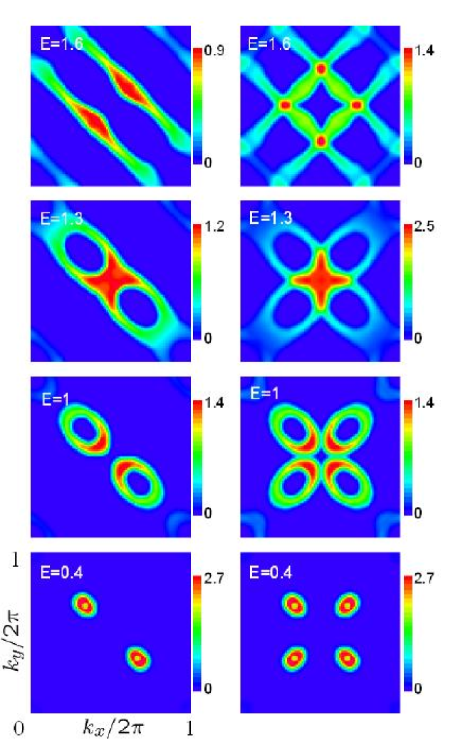
Figure 9: (Color online) DS3 at $J_{b}=0.1J_{a}$: Constant energy cuts with windows of $0.2Ja$ for diagonal, site-centered stripes of spacing $d=3$ at $J_{b}=0.1J_{a}$. The left column is untwinned and the right one is twinned. The energy $E$ is in units of $J_{a}S$.

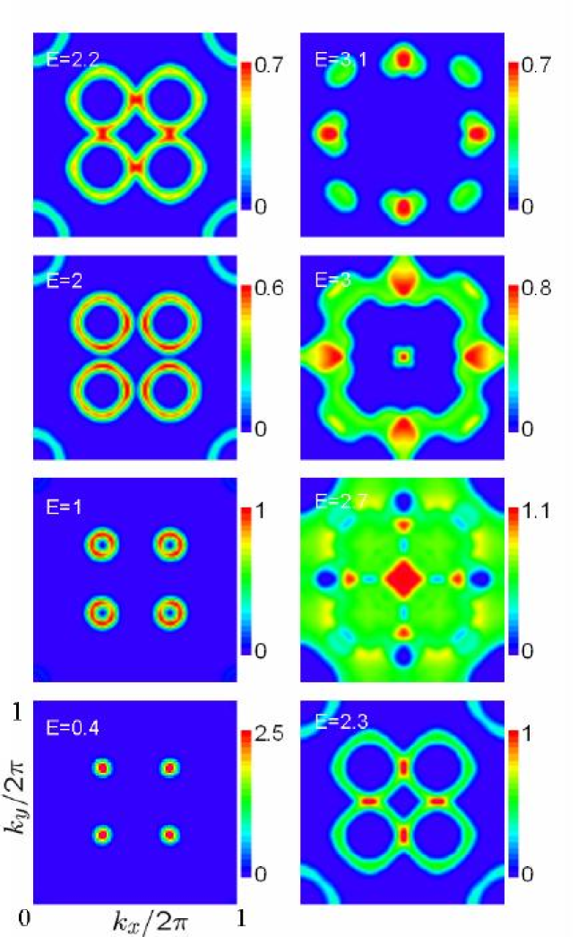
Figure 10: (Color online) DS3 at $J_{b}=0.5J_{a}$: Constant energy cuts with windows of $0.2Ja$ for diagonal, site-centered stripes of spacing $d=3$ at $J_{b}=0.5J_{a}$. Each panel is twinned. The energy $E$ is in units of $J_{a}S$.

(a) DB2 Intensity Ratio

(b) DS3 Intensity Ratio

Figure 11: Intensity ratio between the “inner” and “outer” branches of the spin wave cones as a function of coupling ratio $|J_{b}/J_{a}|$ for diagonal stripes. The solid points are our numerical calculations of the intensity ratio. The solid line is a fit to the results, as explained in the text. (a) DB2: Intensity ratio for diagonal bond-centered stripes of spacing $d=2$ at $E=0.4J_{a}S$. (b) DS3: Intensity ratio for diagonal site-centered stripes of spacing $d=3$ at $E=J_{a}S$.

We now consider diagonal stripes. Diagonal stripes have been observed in the nickelates,tranquadaLSNO ; boothroyd and at low doping in the cuprates, e.g., for $x<0.05$ in La_2-xSr_xCuO₄ (LSCO).wakimoto ; lsco1d When the crystals are detwinned, the diagonal stripe incommensurate peaks are also untwinned in the cuprates.wakimoto ; lsco1d To make a comparison with the experiments on diagonal stripes, we report results for untwinned stripes as well as twinned stripes.

The expected neutron scattering intensities for diagonal stripes depend starkly on whether the stripes have an even or odd spacing. Diagonal bond-centered stripes of odd spacing generally display net ferromagnetism. This is because diagonal bond-centered domain walls have a net magnetic moment, and at odd domain wall spacing, each domain wall will have the same moment. This dramatically changes the nature of the Goldstone modes from linear to quadratic in $|k-k_{o}|$. For site- or bond-centered diagonal stripes of even spacing, the number of magnetic reciprocal lattice vectors doubles, and then even $Q_{AF}=(\pi,\pi)$ is a reciprocal lattice vector. Since stripes are arrays of antiphase domain walls in the antiferromagnetic texture, there can be no net antiferromagnetism, and hence no zero frequency weight at $Q_{AF}$. Nevertheless, a spin wave cone emanates from the $(\pi,\pi)$ point when the diagonal spacing is even. The cone has no weight at zero frequency, and gains a faint appearance as energy is increased.spinprb1 Because of this unique band structure, even-spaced diagonal stripes cannot display a saddlepoint in the acoustic band at $(\pi,\pi)$. There is, however, a saddlepoint in the next optical band.

We show results for diagonal stripes in Figs. 8-11. As with vertical stripes, the intensity profile of the spin wave cones at low energy is a function of $|J_{b}/J_{a}|$. For weak coupling $J_{b}$, the weight is strongly gathered near the $(\pi,\pi)$ point. In Fig. 11, we plot the intensity ratio between the inner and outer branches of the spin wave cones at small energy, for both DB2 (diagonal bond-centered stripes of spacing $d=2$, Fig. 11a) and DS3 (diagonal site-centered stripes of spacing $d=3$, Fig. 11b). To obtain the figures, we have taken a cut through $k$-space perpendicular to the stripe direction, along $(k_{x},-k_{x})$, and we restrict the plots to a low energy, $E=0.4J_{a}S$. We plot the peak intensity at the inner branch of the spin wave cone (toward $(\pi,\pi)$) divided by the peak intensity of the outer branch of the spin wave cone (away from $(\pi,\pi)$). By fitting the results in Fig. 11 for diagonal stripes we find that it is well described by the same functional form that we used for vertical stripes, although the fitted constants are different. Based on a fit to Eqn. 4, we find that for DB2 at $E=0.4J_{a}S$ (Fig. 11a), $a=1.8$, $b=0.022$, $c=0$, and $\mu=2.6$. There is a slight deviation from the fit near $J_{b}=-0.25J_{a}$. For DS3 at $E=J_{a}S$ (Fig. 11b), we find that $a=0.74$, $b=0.15$, $c=-0.11$, and $\mu=0.61$. As with vertical stripes, for diagonal stripes of both the site- and bond-centered type, at small enough coupling ratio $|J_{b}/J_{a}|$, the intensity on the outer branch is so weak that only part of the spin wave cone will be visible without sufficient experimental resolution, indicating that diagonal stripes can also display “legs of scattering” when the spin coupling across the charge stripe is weak. (Similarly, large coupling across the charge stripe can display outwardly dispersing “legs of scattering”.)

In Fig. 8 we show constant energy cuts for DB2, a bond-centered diagonal stripe configuration with spacing $d=2$ between domain walls, at weak coupling across the charge stripes, $J_{b}=-0.1J_{a}$. We report untwinned intensity plots in the left column, and twinned intensity plots in the right column. At low energies, the twinned intensity plots show four spin wave cones dispersing from the incommensurate peaks, with weight concentrated near the $(\pi,\pi)$ point.

At higher energies in Fig. 8, because the stripe spacing $d$ is even, the acoustic band cannot support a saddlepoint at $(\pi,\pi)$, as discussed above. Rather, it is the optical band that has a saddlepoint, appearing at $E=1.4J_{a}S$. Like the resonance peaks in vertical stripes, the saddlepointgruninger has higher intensity, with low energy and high energy branches emanating from it. Due to the weak coupling across charge stripes $|J_{b}|\ll J_{a}$, the high energy branches emanating from the saddlepoint are rather flat, giving rise to a high energy square shaped continuum in the twinned plots, rotated $45^{o}$ from the low energy peaks.

In Fig. 9, we show results for DS3, diagonal site-centered stripes of spacing $d=3$, with $J_{b}=0.1J_{a}$. Because the coupling $J_{b}$ is weak, the spin wave cones have weight gathered near $(\pi,\pi)$. The low energy dispersion for DS3 at this coupling is much steeper than that for DB2 at the same coupling strength, because unlike DB2, DS3 has no magnetic reciprocal lattice vectors at $(\pi,\pi)$, and so the spin wave cones of DS3 continue up in energy to a saddlepoint at $(\pi,\pi)$. The saddlepoint occurs at $E=1.3J_{a}S$, and it has extra intensity when twinned. As with other saddlepoints at low $J_{b}$, there are high energy and low energy branches emanating from it, resulting in an hourglass shape in $E$ vs. $k$ for twinned stripes. The weak coupling $J_{b}\ll J_{a}$ gives rise to a square shaped continuum above the saddlepoint, with vertices rotated $45^{o}$ from the low energy peaks, a familiar pattern at high energy.

In Fig. 10, we show DS3 at higher coupling ratio, $J_{b}=0.5J_{a}$. This pattern and coupling has been shown to capture many essential features of the data for the nickelate compound La_2-xSr_xNiO₄ at $x=1/3$, and to some extent $x=0.275$ as well.tranquadaLSNO To more fully compare with this experiment, we show results only for twinned stripes. Our results may be compared with Figs. $2,~{}5,$ and $10$ of Ref. tranquadaLSNO . (However note that the axes of the plots in Ref. tranquadaLSNO are rotated $45^{o}$ from our plots.) At low energy (up to $E=J_{a}S$), the spin wave cones have intensity peaked on the outer branch. However, at higher energy, $E=2J_{a}S$, the intensity has shifted, and is now peaked on the inner branch. The spin wave cones remain remarkably circular through this energy range, despite the anisotropic coupling ratio. As the spin wave cones touch at $E=2.3J_{a}S$, there are four regions of high scattering radiating out from $(\pi,\pi)$. As the cones merge, they form a central peak at $(\pi,\pi)$, surrounded by four smaller regions of high scattering, rotated $45^{o}$ from the low energy peaks. These four smaller peaks are mainly due to the addition of two twinned stripe patterns. At higher energy, these four peaks move outward (occupying the corners of the graph in Fig. $5$(f) of Ref. tranquadaLSNO ), while the peak at $(\pi,\pi)$ diminishes. Finally at higher energy $E=3.1J_{a}S$, the peak at $(\pi,\pi)$ is no longer visible. This indicates that rather than being a saddlepoint, as happened for $J_{b}\ll J_{a}$, by the time the coupling ratio has reached $J_{b}=0.5J_{a}$, there is no longer a saddlepoint at $(\pi,\pi)$. Rather, there is simply a band edge at $E=3J_{a}S$. This is also consistent with the fact that the $(\pi,\pi)$ peak in this case does not display significantly higher intensity compared to that of nearby energy cuts.

V RESULTS: Spectra of Checkerboards

Figure 12: (Color online) CS3 at $J_{b}=0.1J_{a}$: Constant energy cuts for site-centered checkerboard pattern with stripe spacing $d=3$ at $J_{b}=0.1J_{a}$. The energy $E$ is in units of $J_{a}S$.

We show in Fig. 12 the expected scattering response from a typical simple checkerboard pattern. We show results for a site-centered checkerboard pattern of spacing $d=3$, the real space pattern of which is shown in Fig. 2(a). At low energies, simple checkerboards which use the charged lines as antiphase domain walls in the spin texture yield zero frequency peaks (and therefore low energy spin wave cones) which are in the wrong direction. That is to say, for vertically placed domain walls (as required by both the charge incommensurate peaks in neutron scattering on LNSCO at dopings $x>0.05$tranqnature ; ichikawa and the STM Fourier transform peaks in BSCCOchecknccoc ; aharon ; hoffman ) the spin incommensurate peaks are rotated $45^{o}$ from those observed experimentally.vojta-sachdev Simple checkerboard pattens like these always give IC spin peaks rotated $45^{o}$ from the direction of the charge IC peaks,vojta-sachdev ; andersen03 contrary to what has been seen experimentally. However, more complicated checkerboard patternsabbamonte may be capable of fitting the low energy data, and we plan to explore the finite frequency response of these in a future publication.future

Simple bond-centered checkerboards of odd spacing ($d\in odd$) suffer yet another ill: they support a net magnetization as shown in Fig. 2(b). As a result, they display a ferromagnetic spin peak at $Q_{F}=(0,0)$, and spin waves which are quadratic rather than linear in $|k-k_{o}|$, where $k_{o}$ is a magnetic reciprocal lattice vector. Net ferromagnetism is not attainable for simple vertical stripes, but it is possible with bond-centered diagonal stripes of odd spacing, as discussed in Sec. IV.

The spin wave cones at low energy in Fig. 12 have weight gathered on the inner branches on the side nearest $(\pi,\pi)$. The intensity in these cones merges into a square-like pattern as energy is increased, before the band ends with a peak at $E=1.4J_{a}S$ and $(\pi,\pi)$. The high energy part of the acoustic band also has incommensurate peaks which are in the correct direction for the low energy IC spin peaks, but are overwhelmed in intensity by the central peak at $Q_{AF}$. The high energy peak at $Q_{AF}$ which marks the top of the acoustic band is unlike the resonance peak observed in the experiment, since there is no scattering signal emanating from it at higher energy.vojta-sachdev Rather, above $E=1.4J_{a}S$ in Fig. 12, there is a spin wave gap to a rather flat optical band.

The form of the energy in this checkerboard configuration (CS3) may be calculated analytically. There are four spins in the unit cell, as shown in Fig. 2(a), and only two bands. Along the direction diagonal to the domain walls $(k_{x},k_{x})$, the dispersions for the accoustic and optical bands are

$$\frac{\omega_{acc}}{J_{a}S}=4\sqrt{\lambda}|\sin{\frac{3k_{x}}{2}}|,$$ (5)

$$\frac{\omega_{op}}{J_{a}S}=2(1+\lambda)~{},$$ (6)

with $\lambda=J_{b}/J_{a}$. Notice that the optical band is flat in this direction. Along the direction parallel to the domain walls $(k_{x},0)$, the dispersions are

$$\big{(}\frac{\omega}{J_{a}S}\big{)}^{2}/2 = (1+3\lambda+\lambda^{2}-\lambda\cos{3k_{x}})$$

$$\pm (1+\lambda)\sqrt{1+\lambda^{2}+2\lambda\cos{3k_{x}}}~{},$$

where the $-$ sign refers to the acoustic band, and the $+$ sign refers to the optical band. The spin wave velocities in the diagonal and parallel directions are

$$v_{diag}=\frac{3\sqrt{\lambda}}{2}v_{AF},$$ (8)

$$v_{||}=\frac{3\sqrt{\lambda}}{2\sqrt{2}}v_{AF}~{}.$$ (9)

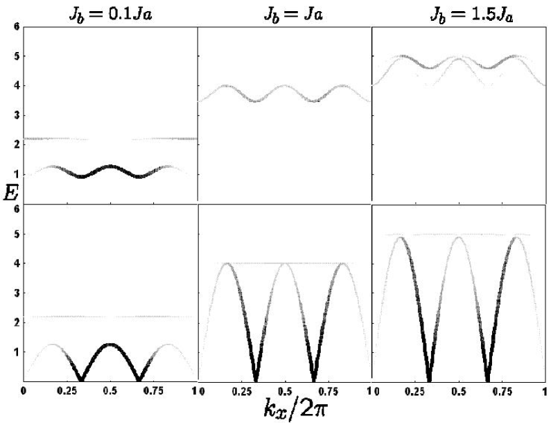
Figure 13: CS3 at $J_{b}=0.1J_{a}$: Dispersion and intensities for a site-centered checkerboard pattern with stripe spacing $d=3$ at $J_{b}=0.1J_{a}$. The upper pannel is along ($k_{x},\pi$) direction ; the lower pannel corresponds to the diagonal direction ($k_{x},k_{x}$). The energy $E$ is in units of $J_{a}S$.

These band structures (with numerically calculated intensities) are shown in Fig. 13 in the $(k_{x},\pi)$ and $(k_{x},k_{x})$ directions. There are always two bands present, although one is often quite weak compared to the other. The coupling at which the two bands touch each other is $J_{b}=J_{a}$. Fig. 13(a) shows the gap that is present between the acoustic and optical bands, and that there is no high energy structure emanating from the peak at $(\pi,\pi)$ which terminates the acoustic band.

VI Conclusions

In conclusion, we have studied the expected inelastic neutron scattering intensities from spin waves for a variety of spin-ordered phases, including vertical and diagonal stripes and a simple checkerboard pattern. We find that the inelastic response is very sensitive to the coupling across domain walls throughout the energy ranges studied. In addition, we wish to emphasize that the elastic response can also hold surprises. For example, we find for vertical stripes of spacing $d=4$ that when the domain walls are site-centered (VS4), the ratio between the main IC peaks and the next satellite peak is at least $34$. This number is independent of coupling strength, and it holds for the most sharply spin-ordered case of a square-wave profile to the antiphase domain walls. Stripes in a real material are expected to have a softer profile due to quantum effects neglected here, and this will diminish the satellite peaks even more. For the bond-centered $d=4$ case (VB4), the satellite peaks are easier to detect, with a ratio of at least $5.9$ between the main IC peaks and the next satellite peaks, even for the most extreme case of a square-wave profile. However, this is still below the noise for current experimental resolution.

For vertical stripes at finite but low energies, the intensity around the spin wave cones is rarely uniform. Rather, it is shifted either toward or away from the $(\pi,\pi)$ point by an amount which depends on the coupling ratio $|J_{b}/J_{a}|$. For weak coupling across the charge stripes, e.g. $|J_{b}|<J_{a}$, the weight is gathered on the inner branch toward the $(\pi,\pi)$ peak, indicating that weak stripe coupling may be responsible for the observed “legs” of scattering in stripe-ordered cuprates at low frequency. For stronger coupling across the charge stripes, e.g. $|J_{b}|>J_{a}$, the intensity shifts to the outer branch. In either case, without sufficient experimental resolution, only part of the spin wave cones will be visible at low energy.

At intermediate energies and for weak coupling, the acoustic band displays a saddlepoint whose intensity profile mimics that of the “resonance peak” observed in cuprate superconductors. For twinned stripes, a saddlepoint displays the characteristic hourglass shape in $E$ vs. $k$ plots seen in some experiments, with both low and high energy legs emanating from a resonance-like peak.mookchg ; ybco6.7 ; ybco ; normanhourglass ; uhrigsaddlepoint

At high energies and weak coupling $J_{b}$, vertical stripes show a square-shaped continuum which is rotated $45^{o}$ from the low energy IC peaks. As we have shown previously,spinprl very weak coupling captures the spin wave excitations of stripe-ordered LBCO at all measured energies, and at higher energies it bears a striking resemblance to the high energy excitations of YBCO. The gap to spin $S=1$ excitations in YBCO is likely due to the stripes being too weakly coupled, and therefore quantum disordered. However, at high energy, the quantum critical excitationsvojta-ulbricht ; uhrig04a ; tranquada04a ; seibold04 strongly resemble the spin waves studied here, which may be due to the proximity of a QCP with small critical exponent $\eta=0.037$.spinprl Near the QCP, one way to distinguish semiclassical spin waves from quantum critical excitations is through the lineshapes. Whereas semiclassical spin waves produce a Lorentzian lineshape, quantum criticality yields a power law cusp. For intermediate and larger couplings $J_{b}$, the high energy response can have a variety of shapes. We have shown here that circular continua are possible, as well as square-shaped continua which either have the same orientation as the low energy peaks, or are rotated $45^{o}$ from that direction.

For diagonal stripes, as with vertical stripes, the low energy spin wave cones have intensity profiles which depend on the strength of the coupling between the stripes. For weak coupling, the intensity is peaked on the inner branches, while for strong coupling, it is peaked on the outer branches. In either extreme case, the entire spin-wave cone may not be visible in an experiment without sufficient resolution. At intermediate energy, weakly coupled diagonal stripes also have a saddlepoint in the acoustic band, with properties akin to the resonance peak. At high energy, weakly coupled diagonal stripes display a high energy square-shaped continuum, rotated $45^{o}$ from the low energy peaks. At higher coupling ratio $|J_{b}/J_{a}|$, the saddlepoint in the acoustic band at $(\pi,\pi)$ is lost, and a variety of high energy scattering patterns are possible. Diagonal bond-centered stripes of odd spacing display net ferromagnetism, changing the nature of Goldstone modes from linear to quadratic in $|k-k_{o}|$. Both site- and bond-centered stripes of even spacing have magnetic reciprocal lattice vectors which include $Q_{\rm AF}=(\pi,\pi)$. Because of the antiphase nature of the domain walls, zero frequency is forbidden at this peak, but the (very low intensity) spin wave cone emanating from $(\pi,\pi)$ precludes a saddlepoint at $Q_{\rm AF}$ in the acoustic band.

For intermediate coupling $J_{b}=0.5J_{a}$, the expected scattering intensity from diagonal, site-centered stripes of spacing $d=3$ strongly resembles that in La_2-xSr_xNiO₄ at $x=1/3$ and $x=0.275$, as pointed out in Ref. tranquadaLSNO . We find for this configuration that while the intensity is peaked on the outer branch of the spin wave cone at low energy, it moves toward the inner branch as energy is increased. Furthermore, the spin wave cones are remarkably circular, despite the anisotropic coupling ratio. With increasing energy, the spin wave cones merge, eventually gathering weight at the central peak $(\pi,\pi)$. However, rather than a saddlepoint, this coupling has a band edge at $(\pi,\pi)$.

Simple checkerboards, on the other hand, have low energy spin IC peaks rotated $45^{o}$ from the observed spin peaks in neutron scattering.vojta-sachdev In addition, for weak coupling across the domain walls $|J_{b}|\ll J_{a}$, rather than showing a resonance-like saddlepoint, the acoustic band has a band edge at $(\pi,\pi)$,vojta-sachdev and therefore no branches emanating from it at high energy. Although the simple checkerboard studied here is incompatible with the experimental data, this does not rule out the possibility of more complicated checkerboard patternsabbamonte which may be able to capture the correct orientation of the low energy spin and charge IC peaks.

References

- (1) T. Hanaguri, C. Lupien, Y. Kohsaka, D. H. Lee, M. Azuma, M. Takano, H. Takagi, and J. C. Davis, Nature 430, 1001 (2004).
- (2) J. E. Hoffman, E. W. Hudson, K. M. Lang, V. Madhavan, H. Eisaki, S. Uchida, and J. C. Davis, Science 295, 466 (2002).
- (3) C. Howald, H. Eisaki, N. Kaneko, and A. Kapitulnik, Proc. Natl. Acad. Sci.U.S.A. 100, 9705 (2003).
- (4) H. A. Mook, P. Dai, and F. Dogan, Phys. Rev. Lett. 88, 097004 (2002).
- (5) J. M. Tranquada, H. Woo, T. G. Perring, H. Goka, G. D. Gu, G. Xu, M. Fujita, and K. Yamada, Nature 429, 534 (2004).
- (6) S. M. Hayden, H. A. Mook, P. Dai, T. G. Perring, and F. Dogan, Nature 429, 531 (2004).
- (7) B. Lake, G. Aeppli, T. E. Mason, A. Schroder, D. F. McMorrow, K. Lefmann, M. Isshiki, M. Nohara, H. Takagi, and S. M. Hayden, Nature 400, 43 (1999).
- (8) N. J. Curro, P. C. Hammel, B. J. Suh, M. Hucker, B. Buchner, U. Ammerahl, and A. Revcolevschi, Phys. Rev. Lett. 85, 642 (2000).
- (9) C. Niedermayer, C. Bernhard, T. Blasius, A. Golnik, A. Moodenbaugh, and J. I. Budnick, Phys. Rev. Lett. 80 3843 (1998).
- (10) C. Stock, W. J. L. Buyers, R. A. Cowley, P. S. Clegg, R. Coldea, C. D. Frost, R. Liang, D. Peets, D. Bonn, W. N. Hardy, and R. J. Birgeneau, Phys. Rev. B 71, 024522 (2004).
- (11) E. W. Carlson, D. X. Yao, and D. K. Campbell, Phys. Rev. B 70, 064505 (2004).
- (12) D. X. Yao, E. W. Carlson, and D. K. Campbell, Phys. Rev. Lett. 97, 017003 (2006).
- (13) M. Vojta and T. Ulbricht, Phys. Rev. Lett. 93, 127002 (2004).
- (14) G. S. Uhrig, K. P. Schmidt, and M. Grninger, Phys. Rev. Lett. 93, 267003 (2004).
- (15) G. Seibold and J. Lorenzana, Phys. Rev. Lett. 94, 107006 (2004).
- (16) M. Vojta and S. Sachdev, J. Phys. Chem. Solids 67, 11 (2006).
- (17) J. M. Tranquada, P. Wochner, A. R. Moodenbaugh, and D. J. Buttrey, Phys. Rev. B 55, R6113 (1997).
- (18) B. M. Andersen, P. Hedegard, and H. Bruus, Phys. Rev. B 67, 134528 (2003).
- (19) P. Abbamonte (private communication).
- (20) A. Auerbach, Phys. Rev. Lett. 72, 2931 (1994).
- (21) F. Krger and S. Scheidl, Phys. Rev. B 67, 134512 (2003).
- (22) P. Wochner, J. M. Tranquada, D. J. Buttrey, and V. Sachan, Phys. Rev. B 57, 1066 (1998).
- (23) G. S. Uhrig, K. P. Schmidt, and M. Grninger, J. Magn. Magn. Mater. 290-291, 330 (2005).
- (24) M. Arai, T. Nishijima, Y. Endoh, T. Egami, S. Tajima, K. Tomimoto, Y. Shiohara, M. Takahashi, A. Garrett, and S. M. Bennington, Phys. Rev. Lett. 83, 608 (1999).
- (25) P. Dai, H. A. Mook, and F. Dogan, Phys. Rev. Lett. 80, 1738 (1998).
- (26) M. R. Norman, Phys. Rev. B 63, 092509 (2001).
- (27) R. Coldea, S. M. Hayden, G. Aeppli, T. G. Perring, C. D. Frost, T. E. Mason, S.-W. Cheong, and Z. Fisk, Phys. Rev. Lett. 86, 5377 (2001).
- (28) K. Yamada, C. H. Lee, K. Kurahashi, J. Wada, S. Wakimoto, S. Ueki, H. Kimura, Y. Endoh, S. Hosoya, G. Shirane, R. J. Birgeneau, M. Greven, M. A. Kastner, and Y. J. Kim, Phys. Rev. B 57, 6165 (1998).
- (29) P. Dai, H. A. Mook, R. D. Hunt, and F. Dogan, Phys. Rev. B 63, 054525 (2001).
- (30) A. V. Balatsky and P. Bourges, Phys. Rev. Lett. 82, 5337 (1999).
- (31) V. Hinkov, S. Pailhes, P. Bourges, Y. Sidis, A. Ivanov, A. Kulakov, C. T. Lin, D. P. Chen, C. Bernhard, and B. Keimer, Nature 430, 650 (2004).
- (32) H. Woo, A. T. Boothroyd, K. Nakajima, T. G. Perring, C. Frost, P. G. Freeman, D. Prabhakaran, K. Yamada, and J. M. Tranquada, Phys. Rev. B 72, 064437 (2005).
- (33) A. T. Boothroyd, D. Prabhakaran, P. G. Freeman, S. J. S. Lister, M. Enderle, A. Hiess, and J. Kulda, Phys. Rev. B 67, 100407(R) (2003).
- (34) S. Wakimoto, J. M. Tranquada, T. Ono, K. M. Kojima, S. Uchida, S. H. Lee, P. M. Gehring, and R. J. Birgeneau, Phys. Rev. B 64, 174505 (2001).
- (35) S. Wakimoto, R. J. Birgeneau, M. A. Kastner, Y. S. Lee, R. Erwin, P. M. Gehring, S. H. Lee, M. Fujita, K. Yamada, Y. Endoh, K. Hirota, and G. Shirane, Phys. Rev. B 61, 3699 (2000).
- (36) U. S. Uhrig, K. P. Schmit, and M. Grninger, J. Phys. Soc. Jpn 74, 86 (2005).
- (37) J. M. Tranquada, B. J. Sternlieb, J. D. Axe, Y. Nakamura, and S. Uchida, Nature 375, 561 (1995).
- (38) N. Ichikawa, S. Uchida, J. M. Tranquada, T. Niemoller, P. M. Gehring, S. H. Lee, and J. R. Schneider, Phys. Rev. Lett. 85, 1738 (2000).
- (39) D. X. Yao, E. W. Carlson, and D. K. Campbell, forthcoming.