Coarse graining the Cyclic Lotka-Volterra Model: SSA and local maximum likelihood estimation.

Abstract

When the output of an atomistic simulation (such as the Gillespie stochastic simulation algorithm, SSA) can be approximated as a diffusion process, we may be interested in the dynamic features of the deterministic (drift) component of this diffusion. We perform traditional scientific computing tasks (integration, steady state and closed orbit computation, and stability analysis) on such a drift component using a SSA simulation of the Cyclic Lotka-Volterra system as our illustrative example. The results of short bursts of appropriately initialized SSA simulations are used to fit local diffusion models using Aït-Sahalia’s transition density expansions ait2 ; aitECO ; aitVEC in a maximum likelihood framework. These estimates are then coupled with standard numerical algorithms (such as Newton-Raphson or numerical integration routines) to help design subsequent SSA experiments. A brief discussion of the validity of the local diffusion approximation of the SSA simulation (a jump process) is included.

1 Introduction

Reactive particle dynamic models arise in scientific fields ranging from physical and chemical processes to systems biology nicolis1 ; nicolis2 ; yanniscatalyst ; VAguy ; doyle ; chemlang ; NatureCircRhythm . Incorporating successive levels of detail in the modeling quickly leads to models that are analytically intractable, necessitating computational exploration. Gillespie’s Stochastic Simulation Algorithm (SSA) and its variants VAguy ; tau2 ; chemlang have gained popularity in recent years for modeling so-called mixed reacting systems; the approach provides a middle ground between detailed molecular dynamics and lumped, Ordinary Differential Equation (ODE) descriptions of chemical kinetics, incorporating fluctuations. Knowing the kinetic scheme underlying such a simulation allows one to write, at the infinite particle limit, the corresponding kinetic ODE. At intermediate particle numbers ($N_{mol}$), the SSA has been approximated with the continuous “chemical Langevin equation” chemlang .

In what follows we will assume that the results of an SSA simulation can be successfully approximated through a continuous diffusion process. Explicit knowledge of the drift and noise components of such a process allows one to easily analyze certain features of the overall behavior; one might, for example, be interested in the bifurcation behavior of the “underlying” drift component of the model, including the number and stability of its steady states and their parametric dependence. In our work we assume that the only available simulation tool is a “black box” SSA simulator, in which the mechanistic rules have been correctly incorporated, but which we, as users, do not know: we can only observe the SSA simulator output. We want to perform a quantitative computational study of the underlying drift component. Since we cannot derive it in closed form (not knowing the evolution rules), we want to perform this study using the least possible simulation with the SSA code. The approach we use follows the so-called “equation-free” framework CommMathSci ; yannisgear : in this framework traditional numerical algorithms become protocols for designing short bursts of numerical experiments with the SSA code. The quantities necessary for numerical computation with the unavailable model (time derivatives, the action of Jacobians) are estimated locally by processing the “fine scale” SSA simulations. In this work we extract such numerical information via parametric local diffusion models using the transition density expansions proposed by Aït-Sahalia aitECO ; aitVEC . The numerical procedures we illustrate can also be used, in principle, for different types of “fine scale” models if their output happens to be well approximated by diffusion processes.

The article is organized as follows: In Section 2 we describe our illustrative model system. We then quickly outline the basic ideas underlying equation-free numerics (Section 3), and discuss our estimation procedure (Section 4). Our computational results are presented in Section 5, and we conclude with a discussion including goodness-of-fit issues.

2 The Lattice Lotka-Volterra Model

Our Cyclic Lotka-Volterra LLV ; durrett illustrative example consists of a three-species ($X$, $Y$ and $S$) nonlinear kinetic scheme of the following form LLV :

$$X\,+\,Y\quad \mathop{\rightarrow}^{k_{1}}\quad 2Y$$

$$Y\,+\,S\quad \mathop{\rightarrow}^{k_{2}}\quad 2S$$

$$S\,+\,X\quad \mathop{\rightarrow}^{k_{3}}\quad 2X.$$

In the remainder of the paper we will refer to it simply as LV. In the deterministic limit, this kinetic scheme gives rise to a set of three coupled nonlinear ODEs for the evolution of the concentrations $X,Y$ and $S$.

$${dX\over dt} = -k_{1}XY+k_{3}XS$$ (1)

$${dY\over dt} = -k_{2}YS+k_{1}YX$$

$${dS\over dt} = -k_{3}SX+k_{2}SY$$

The total concentration ($X+Y+S$) is constant over time; setting (without loss of generality) this constant to unity and eliminating $S$

$$X+Y+S=1,\>\>\>\Longrightarrow\>\>\>S=1-X-Y$$

reduces the system to

$${dX\over dt} = X\left[k_{3}-k_{3}X-(k_{1}+k_{3})Y\right]$$ (2)

$${dY\over dt} = Y\left[-k_{2}+(k_{1}+k_{2})X+k_{2}Y\right].$$

For every (positive) value of $k_{1},k_{2}$ and $k_{3}$ four fixed points exist: three trivial and one non-trivial steady state:

$$X_{s} = 0,\,Y_{s}=0,\,S=1\quad(\rm{system\,invaded\,by\,}S)$$

$$X_{s} = 1,\,Y_{s}=0,\,S=0\quad(\rm{system\,invaded\,by\,}X)$$

$$X_{s} = 0,\,Y_{s}=1,\,S=0\quad(\rm{system\,invaded\,by\,}Y)$$

$$X_{s} = {k_{2}\over{K}},\,Y_{s}={k_{3}\over{K}},S_{s}={k_{1}\over{K}}\quad(\rm{nontrivial\,fixed\,point})$$

where

$$K=k_{1}+k_{2}+k_{3}.$$ (3)

An interesting feature of the phase space of the deterministic model is the existence of a one-parameter family of closed orbits surrounding a “center” (see Figure 3). The neutral stability of these orbits affects, as we will see below, the fixed point algorithms used to converge on them. The system is simulated through both the ODEs (2) and through an SSA implementation of the kinetic scheme (2) using $k_{1},k_{2}=0.5$ and $k_{3}=0.7$ throughout.

3 Equation Free Computation

The basic premise underlying equation-free modeling and computation is that we have available a “black box” fine-scale dynamic simulator, and we believe that an effective evolution equation exists (closes) for some set of (coarse-grained) outputs or observables of the fine scale simulation. As discussed in more detail in yannisgear ; hummer , one can numerically solve this (unavailable explicitly) equation through linking traditional numerical methods with the fine scale code; in particular, the classical continuum algorithms become protocols for the design of short, appropriately initialized numerical experiments with the fine scale code. The process starts by identifying the appropriate coarse-grained observables (sometimes also called order parameters); typically these variables are low-order moments of microscopically/stochastically evolving particle distributions (e.g. concentrations for chemically reacting systems, like our example). In general, good coarse-grained observables are not known, and data analysis techniques to identify them from computational or experimental observations are the subject of intense current research Isomap ; belkin ; PNASCoifman . If the unavailable “effective” equations are deterministic and reasonably smooth, short runs of the fine-scale simulator are used to estimate time derivatives of the coarse-grained observables; initializing fine scale simulations consistent with nearby values of the coarse-grained observables gives estimates of directional derivatives (again assuming appropriate smoothness), and can be linked with matrix-free iterative linear algebra techniques (e.g. kelley ). When an explicit evolution equation is available, these quantities, necessary in numerical computation, are obtained through function or Jacobian evaluations of the model formulas; here, they are estimated on demand from short computational experiments with the fine scale solver. If the underlying effective equation is stochastic, e.g. a diffusion, then the results of the short simulation bursts must be used to estimate both the drift and the noise components of the effective model - this is the case we study here. We will illustrate, using the SSA LV example, how certain types of computations can be accelerated by appealing to classical numerical methods.

4 Estimation Procedure

In what follows, we will assume that species concentrations are good observables, and that the true process (the LV SSA simulation) can be adequately approximated by a diffusion process, that is, a stochastic differential equation (SDE) of the form:

$$d\mathbf{X_{t}}=\mathbf{\mu(X_{t};}\theta)dt+\mathbf{\Sigma(X_{t};}\theta)d\mathbf{W_{t}}.$$ (4)

Here $\mathbf{X_{t}}$ is a stochastic process which is meant to model the evolution of the observable(s), $\mathbf{W_{t}}$ represents a vector of standard Brownian motions, and the functions $\mathbf{\mu(X_{t};}\theta)$ and $\mathbf{\Sigma(X_{t};}\theta)$ are the drift and diffusion coefficients of the process. In the classical parametric setup, one assumes that the parameterized function families to which the drift and diffusion coefficient functions belong are known, and that the parameter vector $\theta$ is finite dimensional. In practice one rarely knows a class of functions which can be used to describe the global dynamics of the observables; in the equation free computations below, however, we simulate the true process for only relatively short bursts of time. It therefore makes sense to (locally) consider the following SDE:

$$d\mathbf{X_{t}}=\Big{(}\mathbf{A}+\mathbf{B(X_{t}-X_{o})}\Big{)}dt+\Big{(}\mathbf{C+D(X_{t}-X_{o})}\Big{)}d\mathbf{W_{t}}.$$ (5)

where $\mathbf{W_{t}}$,$\mathbf{X_{t}}$,$\mathbf{X_{o}}$, $\mathbf{A}$ and $\mathbf{C}$ $\in\mathbb{R}^{d}$ and $\mathbf{B}$ and $\mathbf{D}$ $\in\mathbb{R}^{d\times d}$ (the $d$ Brownian motions are assumed independent; the vector multiplying them, by slight abuse of notation, contains the nonzero elements of the diagonal matrix $\mathbf{\Sigma}$; extending to the correlated case is straightforward).

This simple model is based on the fact that we expect smooth evolution of moments of the observables, while at the same time taking into account the state dependence of the noise (neglecting this dependence can cause bias in the estimation of the drift). The parameters of this local linear model are estimated through techniques associated with maximum likelihood estimation (MLE). The motivation for using MLE techniques stems from the fact that under certain regularity conditions vandervaart such estimators are (asymptotically) efficient as regards the variance of the estimated parameter distribution. In addition, the asymptotic parameter distributions associated with MLE can sometimes be worked out analytically, or approximated through Monte Carlo simulations; this knowledge can guide the selection of the sample size necessary for a given desired accuracy in coarse-grained computations llglassy .

4.1 Maximum Likelihood Estimation for Discretely Observed Diffusions

We now recall a few basic facts about MLE estimation; standard references include, e.g. hamilton ; jeganathan ; vandervaart . It is assumed throughout that the exact distribution associated with the parametric model admits a continuous density whose logarithm is well defined almost everywhere and is three times continuously differentiable with respect to the parameters kl .

MLE is based on maximizing the log-likelihood ($\mathcal{L}_{\theta}$) with respect to the parameter vector (for our model $\theta\equiv[\mathbf{A},\mathbf{B},\mathbf{C},\mathbf{D}]$):

$$\mathcal{L}_{\theta}\equiv\log\Big{(}f(\mathbf{x};\theta)\Big{)}.$$ (6)

In the above equation, $\mathbf{x}$ corresponds to a matrix of observations $\in\mathbb{R}^{d\times M}$ where $d$ is the dimension of the state and $M$ is the length of the time series; $f(\mathbf{x};\theta)$ corresponds to the probability of making observation $\mathbf{x}$. For a single sample path of a discretely observed diffusion known to be initialized at $\mathbf{x}_{0}$, $f(\mathbf{x};\theta)$ can be evaluated as hamilton :

$$f(\mathbf{x};\theta)=\delta_{{x}_{0}}\prod\limits_{m=1}^{M-1}f(\mathbf{x}_{m}|\mathbf{x}_{m-1};\theta).$$ (7)

In this equation $f(\mathbf{x}_{m}|\mathbf{x}_{m-1};\theta)$ represents the conditional probability (transition density) of observing $\mathbf{x}_{m}$ given the observation $\mathbf{x}_{m-1}$ for a given $\theta$ and $\delta_{{x}_{0}}$ is the Dirac distribution. In our applications, we search for the parameter vector that is best over all observations (we have an ensemble of $N$ paths of length $M$). In this case our expression for the log-likelihood (given the data and transition density) takes the form:

$$\mathcal{L}_{\theta}:=\sum\limits_{i=1}^{N}\sum\limits_{m=1}^{M}\log\Big{(}f(\mathbf{x}_{m}^{i}|\mathbf{x}_{m-1}^{i};\theta)\Big{)}.$$ (8)

Assume the existence of an invertible symmetric positive definite “scaling matrix” matrix $\mathcal{F}_{(M,\ \theta)}$ lecam00 associated with the estimator; the subscripts are used to make the dependence of the scaling matrix on $M$ and $\theta$ explicit. For the “standard” case $N=1$ in time series analysis, under some additional regularity assumptions jeganathan ; vandervaart , one has the following limit for a correctly specified parametric model:

$$\mathcal{F}_{(M,\ \hat{\theta})}^{\frac{1}{2}}(\theta_{M}-\hat{\theta})\stackrel{{\scriptstyle\mathbb{P}_{\hat{\theta}}}}{{\Longrightarrow}}N(\mathbf{0},\mathbf{I}).$$ (9)

Here $\hat{\theta}$ is the true parameter vector; $\theta_{M}$ represents the parameters estimated with a finite time series of length $M$; $\stackrel{{\scriptstyle\mathbb{P}_{\hat{\theta}}}}{{\Longrightarrow}}$ denotes convergence in distribution vandervaart ; hamilton under $\mathbb{P}_{\hat{\theta}}$ (the distribution associated with the density $f(\mathbf{x};\hat{\theta)}$); $N(\mathbf{0},\mathbf{I})$ denotes a normal distribution with mean zero and an identity matrix for the covariance. For a correctly specified model family, $\mathcal{F}_{(M,\ \hat{\theta})}$ can be estimated in a variety of ways white ; lecam00 . The appeal of MLE lies in that, asymptotically in $M$, the variance of the estimated parameters is the smallest that can be achieved by an estimator that satisfies the assumed regularity conditions jeganathan ; vandervaart .

4.2 Transition density expansions

Here we briefly outline the key features of the recent work of Aït-Sahalia aitECO ; aitVEC used in our coarse-grained computations below. The problem with using even a simple model like that given in equation 5 is that the transition density associated with the process is not known in closed form. In recent years, many attempts to approximate the transition density have appeared in the literature; some techniques depend on analytical approximations whereas others are simulation based (see, e.g. ait2 ; aitECO ; aitextension ; bibby ; gallant ; smle ). We have used, with some success, the expansions found in ait2 ; aitVEC ; aitECO . High accuracy can be obtained using this method to approximate the transition density associated with a scalar process; the multivariate case is discussed in aitVEC . The basic idea behind the scalar case, presented in ait2 ; aitECO , is as follows: One first transforms the process given in equation 4 into a new process aitECO :

$$dY_{t}=\mu_{Y}(Y_{t};\theta)dt+dW_{t}$$ (10)

$$Y\equiv\gamma(X;\theta)=\int^{X}\frac{du}{\sigma(u,\theta)}$$

$$\mu_{Y}(y;\theta)\equiv$$ (11)

$$\frac{\mu(\gamma^{-1}(y;\theta);\theta)}{\sigma(\gamma^{-1}(y;\theta);\theta)}-\frac{1}{2}\frac{\partial\sigma}{\partial x}(\gamma^{-1}(y;\theta);\theta)$$

An additional change of variables brings the transition density of the process closer to a standard normal density $Z\equiv\Delta^{-\frac{1}{2}}(Y-y_{o})$ where $\Delta$ is the time between observations. The transformations introduced allow the use of a Hermite basis set in order to approximate the transition density of the original process via the following series:

$$p_{Z}(\Delta,z|y_{o};\theta)\approx$$

$$\phi(z)\sum\limits_{j=0}^{K}\eta_{Z}^{(j)}(\Delta,y_{o};\theta)H_{j}(z)$$

$$\eta_{Z}^{(j)}(\Delta,y_{o};\theta)\equiv$$ (13)

$$\frac{1}{j!}\int\limits_{-\infty}^{\infty}H_{j}(z)p_{Z}(\Delta,z|y_{o};\theta)dz:=$$

$$\frac{1}{j!}\mathbb{E}[H_{j}\Big{(}\Delta^{-\frac{1}{2}}(Y_{t+\Delta}-y_{o})\Big{)}|Y_{t}=y_{o};\theta]$$

In the above, $H_{j}$ represents the $j^{th}$ Hermite polynomial and $\phi(\cdot)$ is the standard normal density. The coefficients needed for the approximation are obtained through the conditional moments of the process $Y_{t}$. Aït-Sahalia outlines aitECO a procedure which exploits the connection between the SDE and the associated Kolmogorov equations in order to develop a closed form expression for the $\eta_{Z}^{(j)}$ coefficients. The approximation is exact if $K\rightarrow\infty$ and the coefficient functions satisfy the assumptions laid out in aitECO . In numerical applications one must always deal with a finite K. Problems may arise in the truncated expansion: the approximation of the density may not normalize to unity or, worse, it may become negative (see aitVEC ; ait2 ; aitextension for some possible remedies).

In the multivariate case, it becomes more difficult to introduce an analog of $Y_{t}$ aitVEC . Nonetheless, it is still possible to construct a series motivated by the methodology used in the scalar case; however, one now needs to expand in space and time, whereas the Hermite expansion yielded a series “in time only” aitVEC ). Aït-Sahalia aitVEC outlines an approach which makes use of a recursion for calculating the coefficients of the expansion in the multivariate case. We have had success in using these expansions, even in cases where convergence of the infinite series is not guaranteed by the conditions given in ait2 ; aitECO . Notice, for example, that our local models may allow a value of zero for the diffusion coefficient; using a different function class (made computationally feasible by the extension of Bakshi and Ju aitextension ; bakshi05 ), such as sigmoidal functions for it, may help circumvent such problems. Other pathologies are discussed in llglassy ; estimates of the range of the parameters of interest lecam00 ; vandervaart ; llglassy can enhance the algorithm performance. The comparison study jensen_poulsen recommends the use of the expansions by Aït-Sahalia for a wide class of diffusion models. Beyond the estimation itself, these expansions can also be helpful in obtaining diagnostics that depend on knowledge of the transition density (such as goodness-of-fit tests hong ) and asymptotic error analysis lecam00 .

5 Illustrations of Equation-free Computation

Having estimated the parameters of a local model at a given state point opens the way to several computational possibilities. Such estimates, for example, can be used in an iterative search for zeroes of the (global, nonlinear) drift. A Newton-Raphson iteration for a (hopefully better) guess of this root involves the solution of set of linear equations for which both the matrix and the residual are available from the local linear drift. The resulting estimate of the root is then used to launch a new set of computational experiments with the “inner” SSA code, followed by a new estimation, linear equation solution, and so on to convergence. This illustrates the fundamental underpinnings of equation-free computation. Many numerical algorithms (here, root finding through Newton iteration) do not really require good closed-form global models: each iteration only requires local information (the first very few terms of a Taylor series) in order to “design” the next iteration. Traditional continuum numerical methods can thus be thought of as protocols for the design of a sequence of model evaluations (possibly model and Jacobian evaluations, occasionally even Hessian evaluations). In the absence of an explicit formula for the model, the same protocol can be used to design appropriately initialized computational experiments with a model of the system at a different level (here, the SSA simulator). Processing the results of these appropriately initialized short bursts estimate the quantities required for scientific computation, as opposed to evaluating them from a closed-form model. The so-called “coarse projective integration” is another example of the same principle. Traditional explicit integration routines require a call to a subroutine that evaluates the time-derivative of a dynamic model at a particular state. In the absence of an explicit model, short bursts of simulations of a model of the system at a different level (again, here, SSA) can be used to estimate these time derivatives, and, through local linear models, extrapolate the state at a later time. The fundamental assumption underpinning this entire computational framework, is that an explicit evolution equation exists, and closes, in terms of the (known) coarse-grained observables of the fine-scale simulation (here, the concentrations of the SSA species). If this, unavailable in closed-form, equation is deterministic, then one only need to estimate a drift term from fine scale simulations; if, on the other hand, the coarse-grained equation is stochastic (fluctuations are important), then both the local drift and diffusion terms must be estimated. Certain computational tasks for stochastic effective, coarse-grained models require evaluations of both these terms (e.g. computations of stationary, equilibrium densities, or Kramers’ type computations of escape times for bistable systems, see for example dima ; hummer ). In this paper, we perform equation-free tasks for only the drift component of the model; sometimes it may be interesting to know whether the drift component dynamics possess zeros or closed loops, as well as their parametric dependence. Also, at infinite system size (practically, for sufficiently large particle numbers) the SSA actually closes as a deterministic ODE.

Coarse Newton-Raphson for the fixed point of the drift.

In what follows we work at system sizes large enough that a diffusion approximation of the SSA output is meaningful, and -even more- the dynamics of the drift component of the diffusion are close to the kinetic ODE scheme dynamics. The neutral stability of the fixed point and the closed loops of the kinetic ODE suggest comparable features for the estimated drift, which we set out to investigate. We find the nontrivial root of the estimated drift $\mathbf{F(X;}\theta)=\mathbf{0}$ through a coarse Newton-Raphson procedure as follows: An ensemble of $N_{path}$ SSA simulations are initialized in a neighborhood of the current guess $\mathbf{X}_{0}$ of the root. Each is evolved in time, and the simulations are sampled uniformly $M$ times during a time interval of length $\tau$. A local SDE model of the type (5) is estimated using the transition density expansions of Aït-Sahalia in an MLE-type scheme; the resulting model parameters are used to update the root guess through

$$\mathbf{X}_{n}=\mathbf{X}_{n-1}-\frac{\partial\mathbf{F}(\mathbf{X};\theta)}{\partial\mathbf{X}}^{-1}|_{\mathbf{X}=\mathbf{X}_{n-1}}\mathbf{F}(\mathbf{X}_{n-1};\theta)\approx\mathbf{X}_{n-1}-\mathbf{B}^{-1}\mathbf{A}.$$ (14)

Figure 1 shows this procedure for two different values of $N_{path}$ (other parameters are noted in the caption). Newton-Raphson type procedures for isolated roots are known to converge quickly given a good initial guess; furthermore, upon convergence, the eigenvalues of the linearization of the drift are contained in the matrix $\mathbf{B}$. Estimates of these eigenvalues for different $N_{path}$ are listed, upon convergence of the root finding procedure, in Table 1. The equation-free iterates approach the deterministic ODE root (see inset); the latter is known to possess two pure imaginary eigenvalues. The estimated (from local models) eigenvalues are also characterized by a relatively small $(O(10^{-2}))$ real part.

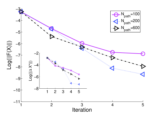
Figure 1: Coarse NR to find stationary points. Roots of $\mathbf{F(X)}\equiv\frac{\mathbf{dX}}{dt}$ using estimated (local) linear SDEs. Parameters: $N_{mol}=1\times 10^{4}$, $\tau=5.032928126\times 10^{-1},M=300$. $N_{path}$ values are shown in the legend and the $l^{2}$ distance of the current guess from the deterministic ODE root is shown in the inset. $\Delta\mathbf{X}^{*}$ (inset y-axis) represents the difference between the current guess and the steady state of the ODE.

Table 1: Representative real and imaginary parts of the eigenvalues of the estimated drift upon convergence to the nontrivial fixed point $\mathbf{X}\approx(0.2941,0.41176)$; the deterministic ODE solution has a pair of pure imaginary eignenvalues.

	Re	Im
$N_{path}=100$	$-2.53\times 10^{-2}$	$3.01\times 10^{-1}$
$N_{path}=600$	$-2.39\times 10^{-2}$	$2.63\times 10^{-1}$

Coarse Projective Integration for the drift

A variety of numerical integration algorithms can be implemented in our framework. Single step methods of the general form

$$\mathbf{X}_{n}=\mathbf{X}_{n-1}+\mathbf{\Phi(X}_{n-1},\mathbf{X}_{n};\Delta t).$$ (15)

include the explicit and implicit Euler algorithms, (for which $\mathbf{\Phi}$ is $\Delta t\mathbf{F(X}_{n-1})$ and $\Delta t\mathbf{F(X}_{n})$ respectively). Estimates of the drift at $\mathbf{X}_{0}$ can be immediately used in a “coarse forward Euler”, while the estimated $\mathbf{B}$ can be used in a root-finding procedure, along the lines illustrated above, in a “coarse backward Euler” scheme. Other schemes can be simply implemented. Here we only demonstrate (explicit) coarse forward Euler; predictor-corrector schemes (more appropriate for stiff problems) are illustrated in llalber . Representative results for our LV problem are shown in Figure 2. The deterministic ODE trajectory (dashed lines connecting points) is compared to the projective integration of the drift component of an SDE estimated locally from SSA simulation ensembles. One clearly sees the evolution of the ensemble of SSA trajectories initialized at every numerical integration point; $N_{path}$ such trajectories were evolved and observed uniformly $M$ times over a time interval $\tau$. The results were processed through the estimation scheme and the value of the drift at the original point $\mathbf{X}_{0}$ provided the forward Euler estimate of the “next” point through $\mathbf{X}_{1}=\mathbf{X}_{0}+\Delta t\mathbf{F}(\mathbf{X}_{0})$. The procedure is then repeated.

Several algorithmic parameters must be carefully selected in such computations. In our case the “lifting” problem (the initialization of SSA simulations at a given value of the coarse observables) is straightforward because of the “mixed” nature of the SSA simulation; in general, the successful initialization of a fine scale code consistent with a few coarse observables can be a complicated and difficult issue, requiring, for example, preparatory constrained dynamic runs Berendsen ; Torrie .

Another important parameter is the length of the integrator “projective” step, $\Delta t$, which for deterministic problems is set by stability and accuracy considerations. Stability discussions for projective integration can be found in CommMathSci ; here the issue is complicated by the fact that the model is estimated rather than evaluated. Multiscale methods for SDEs, including error estimates, can be found in the work of Eijnden ; ELiuEijnden . The total “microscopic integration time” denoted by $\tau$ and the time between observations $\equiv\delta t:=\frac{\tau}{M}$ also require careful selection. If $\tau$ is too large, the simple linear model may break down as nonlinearities in the real system manifest themselves. If the assumed diffusion model is correct, there is no upper limit on $M$; yet a diffusion approximation of a different underlying process, such as the jump SSA here, will break down if the data is sampled too frequently. Similar issues have been addressed in the control literature twoscale . Later on we will outline a goodness-of-fit test that can be used to guide the selection of such algorithmic parameters. In this work, short SSA trajectories in each ensemble are initialized at the same base point $\mathbf{X}_{0}$, or uniformly in a small neighborhood around it; we have not yet explored optimal initialization.

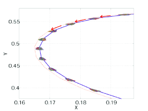
Figure 2: Illustration of Coarse Projective Integration. $N_{path}=600$, $N_{mol}=1\times 10^{4}$, $\Delta t=.50329$, $\tau=\frac{\Delta t}{4}$.

Equation-Free Coarse Variational Calculations

A slight extension of the above coarse integration procedure is the implementation of equation free integration of variational equations. The need for these arises naturally in our example when we attempt to construct an algorithm that searches for possible closed orbits in the dynamics of the estimated drift, and attempts to converge on them. Closed orbits that are limit cycles can be found as (isolated) fixed points of an appropriate Poincaré map. In the deterministic LV problem, however, one has a one-parameter family of such orbits, and the fixed points of the Poincaré map are not isolated. Anticipating a family of such closed orbits for our estimated drift model, we isolate a single orbit from this one-parameter family by selecting its period (the Poincaré return time).

For a deterministic model, the initial value problem for the variational equations is

$$\frac{d\mathbf{X}}{dt}=\mathbf{F(X;}\theta)$$ (16)

$$\mathbf{X}(t=0)=\mathbf{X^{IC}}$$

$$\frac{d\mathbf{V}}{dt}=\frac{\partial\mathbf{F(X;}\theta)}{\partial\mathbf{X}}\cdot\mathbf{V}$$

$$\mathbf{V}(t=0)=\mathbf{I}.$$

If $\mathbf{X}\in\mathbb{R}^{d}$ then $\mathbf{V}\in\mathbb{R}^{d\times d}$. We use the results of integrating such variational equations to locate closed orbits as zeroes of the equation $\mathbf{G(X)\equiv X-\Phi_{\tau}(X)}$ where $\mathbf{\Phi}_{\tau}(\cdot)$ represents the result of integration from the (deterministic) initial condition $\mathbf{X}^{IC}$ for time $\tau$. To isolate the zeroes we seek, we select a Poincaré plane through the value $X_{P}=0.3$ of the first coordinate, and the return time; we thus have one equation with one unknown, the $Y$ coordinate of the intersection of our particular closed orbit with the chosen Poincaré plane. For our coarse integration, the return time $\tau$ is typically too large to permit a single local diffusion model to accurately describe the dynamics; we therefore use the following procedure:

• Specify $\tau$ and the number $N_{grid}$ of local models we will use along the orbit, each valid for $T_{f}^{macro}:=\frac{\tau}{N_{grid}}$.

• Simulate $N_{path}$ SSA trajectories starting at the current fixed point guess; use the data as above to estimate the first local linear model. Use its drift (and the matrix ${\mathbf{B}}$) to obtain the next “base point” as well as to step the variational equations for time $T_{f}^{macro}$.

• Repeat $N_{grid}$ times (see Figure 3).

The output of this procedure gives us the residual of the fixed point equation we wish to solve; the results of the variational integration at time $\tau$ (which, upon convergence, will give us an estimate of the monodromy matrix) are then used to compute the Jacobian of the fixed point scheme. One Newton-Raphson step for the $Y$ coordinate of the fixed point is taken, and the procedure is then repeated. Representative numerical results are shown in Figure 4. Because of the neutral dynamics, the eigenvalues of the monodromy matrix upon convergence are both equal to 1 (in the deterministic ODE). Table 2 shows representative eigenvalue upon convergence for different $N_{path}$ (sometimes the eigenvalues are numerically found as complex conjugates with a small imaginary part). Clearly, in addition to the algorithmic parameters involved in coarse projective integration, we should now also take into account the desired accuracy of the variational integration (quantified in part by the existence of an eigenvalue equal to unity upon convergence).

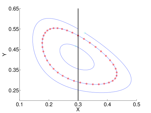
Figure 3: Coarse closed orbit computations for the Lotka Volterra model. The deterministic model phase portrait contains an infinite number of closed orbits. Three such deterministic orbits (obtained by Runge-Kutta integration) are plotted here. To find the closed orbit with a specified period $\tau$, we use the Poincaré surface $X_{P}=0.3$, shown as a solid line. The Jacobian of the coarse Newton-Raphson scheme is computed through variational integrations based on the estimated drift from ensembles of SSA simulations initialized at the $N_{grid}$ base points shown (see text).

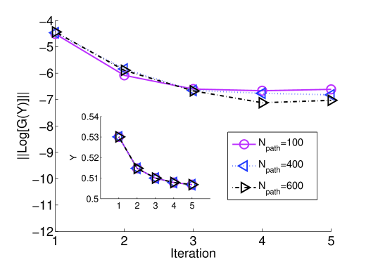
Figure 4: Coarse Newton-Raphson for finding closed orbits of a specified period. The zeroes of $G(Y)\equiv Y-\Phi_{\tau}(Y)$ were calculated using a Jacobian evaluated from coarse variational integration based on SSA simulations. Parameters: $N_{mol}=1\times 10^{4}$, $\tau=2.0131712504\times 10^{1},M=300$, $N_{grid}=40$ ($N_{path}$ given in the legend). The initial guess was $Y=0.53$. For the deterministic ODE model the fixed point is $Y^{ODE}\approx 0.518$; the coarse fixed point for $N_{path}=400$ was calculated to be $Y^{SSA}\approx 0.5075$.

Table 2: Representative monodromy matrix eigenvalues upon convergence of the fixed point iteration for two distinct $N_{path}$ computations (see text).

$N_{path}=100$	$(0.9698,0.1707)$	$(0.9698,-.1707)$
$N_{path}=400$	$(0.9159,0.0252)$	$(0.9159,-.0252)$

6 Discussion

We have illustrated the implementation of certain coarse-grained computations with the LV model; one focus was the coarse-grained integration of the variational equations for the SSA-based drift estimation, as well as the modifications of the coarse Newton-Raphson iteration dictated by the neutral stability of the dynamics (the existence of infinitely many closed orbits in the ODE limit, which appears to approximately persist in our computations). The second focus was the use of Aït-Sahalia’s expansions to estimate local linear SDEs from short bursts of SSA data as an intermediate step. This naturally leads to some crucial questions about the goodness-of-fit of the simple SDE models: (a) is the diffusion approximation a “good” description of the dynamics? (b) Is the linear approximation valid for the time series length chosen? and (c) How reliable is the model for making predictions/forecasts ?

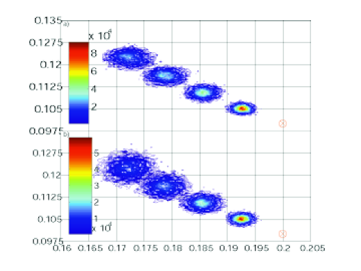
Figure 5: Evolution of actual and model densities. The top figure shows the evolution of the SSA process, initialized as a Dirac distribution (marked in red); the bottom plot shows an ensemble of numerical simulations of the ideal diffusion model using the parameters estimated from the SSA. Both distributions are plotted at $\frac{\tau}{4},\frac{\tau}{2},\frac{3\tau}{4}$,and $\tau$. Relevant parameters: $N_{path}=5\times 10^{3},M=300$, $N_{mol}=1\times 10^{4}$, $\tau=0.50329$.

One should quantitatively know how large $N_{mol}$ needs to be, for a given sampling frequency, for a diffusion model to be a statistically meaningful approximation kurtz05 ; chemlang . Sampling too often may be detrimental in many diffusion approximations (e.g. twoscale ). Local linear models (i.e. short truncations of Taylor series) are used extensively in scientific computations, but only for short time steps, whose length is determined by overall stability and accuracy considerations. Similar considerations arise in choosing the $\tau$ used for SSA data collection towards the estimation of the local linear SDE models used here; clearly, when the underlying drift is nonlinear, $\tau$ cannot be too large. A useful diagnostic tool for questions (a) and (b) applicable if one does have an accurate transition density approximation, is the probability integral transform diebold ; hong . Using the data and the (assumed known) exact transition density, one creates a new random variable which, for a correctly specified model, has a known distribution. The method is applicable to both stationary and non-stationary time series; furthermore it depends on integrations of the transition density approximation rather than differentiations. Given the data, one (appropriately) estimates model parameters and then constructs the random variables $Z_{n}$ for each observation ($x_{n}$). The construction below follows that in Section 3 of diebold :

$$Z_{n}:=\int\limits_{-\infty}^{x_{n}}p(x_{n}^{\prime}|x_{n-1};\theta)dx_{n}^{\prime}$$

$$Z_{n}\sim q(Z_{n})\equiv\frac{d\mathbb{Q}(Z_{n})}{dZ_{n}}$$

$$x_{n}\sim f(x_{n}|x_{n-1})\equiv\frac{d\mathbb{F}(x_{n}|x_{n-1})}{dx_{n}}$$

The symbol $\sim$ denotes that the random variable on the left of the symbol is distributed according to the density to the right. Under a correctly specified model, the $Z_{n}$’s are independent and uniformly distributed on $[0,1]$, independent of the transition density diebold . In hong a comprehensive suite of statistical tests are reviewed which exploit knowledge of the transition density and the transformation shown above. Figure 6 plots a kernel density estimate (see equation 6 on page 44 in hong ) which is based on the estimated parameters and the observed data. If the model is correctly specified, the infinite sample size density should be the product of two uniform densities. Test statistics can be created from this function (see hong for details).

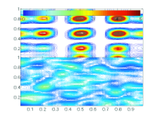
Figure 6: Towards hypothesis testing. The function plotted corresponds to an empirical estimate of the two-dimensional density function described in diebold ; hong . The data are obtained from the same ensemble of SSA simulations as in Fig 5; the top figure is for $N_{mol}=1\times 10^{4}$ and the bottom for $N_{mol}=4\times 10^{5}$. In the infinite sample limit and for a correctly specified model the density would be unity in the entire support ($[0,1]\times[0,1]$) of the function. The figure suggests that the observations of the larger system are closer to a diffusion model.

Inspection of the figures shows that, for a particular representative SSA ensemble run for $N_{mol}=1\times 10^{4}$, and a particular sampling frequency, the diffusion approximation is not acceptable; the situation appears better for $N_{mol}>4\times 10^{5}$. It is interesting to notice that, while $N_{mol}=1\times 10^{4}$ is not large enough for the conditions of Figure 5, visual inspection of the empirical and the SDE-based density evolution might suggest otherwise. In traditional, continuum numerical algorithms issues of on-line error estimation, time-step and mesh adaptation are often built-in in modern, validated software. There is a clear necessity for incorporating, in the same spirit, hypothesis testing techniques in codes implementing the type of computations we described here; yet automating such processes appears to be a major challenge.

In our next application, we evolved an ensemble of trajectories starting from a Dirac initial distribution, and then recorded the Poincaré map for each individual trajectory over a long simulation period. Figure 7 shows the evolution of the $Y$ coordinate of these trajectories as function of the map iterate. For long times, different initial conditions in the ensemble approach some of the “extinction” fixed points of the ODE vector field (see the vertical lines in Fig. 7); once there, the system no longer changes over time. Visual inspection of the evolution of the ensemble suggests that one might try to coarse-grain the Poincaré map evolution as a model SDE; the insets in the figure show the initial evolution of the mean and the variance of the Poincaré map iterates. The smooth line in the insets, a simple least squares fit, seems to suggest a systematic evolution towards “larger” oscillations, bringing the system closer to extinction. If this evolution could be well approximated locally by a diffusion processes, approximations similar in spirit to the ones shown in this article might be used to explore features of the distribution of extinction times for the problem.

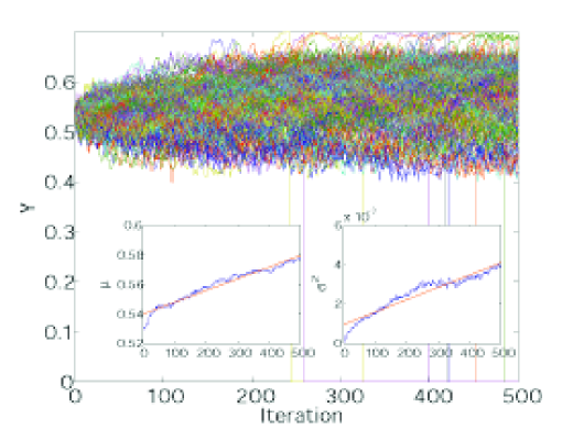
Figure 7: SSA return map computations for the LV model. An ensemble of 200 trajectories initialized at $\mathbf{X}=(0.3,0.53)$ are evolved, and the $Y$ coordinate of their $X_{P}=0.3$ Poincaré map crossings in the negative $X$ direction is recorded. The insets (see text) suggest a systematic upward drift, bringing the system closer to extinction (this event is indicated by vertical lines, see text).

Acknowledgements This work was partially supported by a Ford Foundation/NRC Fellowship to (CC) and an NSF ITR grant (IK).

References

- (1) Y. Aït-Sahalia, Closed-form likelihood expansions for multivariate diffusions, http://www.princeton.edu/~yacine/research.htm, (2001).
- (2) , Maximum-likelihood estimation of discretely-sampled diffusions: A closed-form approximation approach, Econometrica, 70 (2002), pp. 223–262.
- (3) Y. Aït-Sahalia and R. Kimmel, Estimating affine multifactor term structure models using closed-form likelihood expansions, NBER Technical Working Papers 0286, National Bureau of Economic Research, Inc, Dec. 2002. available at http://ideas.repec.org/p/nbr/nberte/0286.html.
- (4) A. Amadei, A.B.M. Linssen, and H.J.C. Berendsen, Essential dynamics of proteins, Proteins, 17 (1993), pp. 412–425.
- (5) G. Bakshi and N. Ju, A refinement to Aït-Sahalia’s (2002) “Maximum likelihood estimation of discretely sampled diffusions: A closed-form approximation approach”, Journal of Business, 78 (2005), pp. 2037–2052.
- (6) G. Bakshi, and N. Ju, and H. Ou-Yang, Estimation of continuous-time models with an applications to equity volatility dynamics (working paper).
- (7) K. Ball, and T. Kurtz, and L. Popovic, and G. Rempala, Asymptotic analysis of multiscale approximations to reaction networks, http://www.citebase.org/cgi-bin/citations?id=oai:arXiv.org:math/0508015, 2005.
- (8) M. Belkin, and P. Niyogi: Laplacian eigenmaps and spectral techniques for embedding and clustering,Advances in Neural Information Processing Systems, vol. 4, edited by S. Becker, and Z. Ghahramani (MIT Press, Cambridge, MA 2002)
- (9) B.M. Bibby and M. Sørensen, Martingale estimation functions for discretely observed diffusion processes, Bernoulli, 1 (1995), pp. 17–39.
- (10) C.P. Calderon and I.G. Kevrekidis, Estimation strategies in equation free numerical methods (in preparation).
- (11) C.P. Calderon, Fitting effective diffusion models to data associated with a “glassy potential”: Estimation, classical inference procedures and some heuristics, http://www.citebase.org/cgi-bin/citations?id=oai:arXiv.org:cond-mat/0510521 (submitted to SIAM MMS) , 2005.
- (12) R.R. Coifman, S. Lafon, A.B. Lee, M. Magionni, B. Nadler, F. Warner, and S.W. Zucker, Geometric diffusions as a tool for harmonic analysis and structure definition of data: Multiscale methods, PNAS, 21 (2005), pp. 7432–7437.
- (13) F.X. Diebold, T. Gunther, and A. Tay, Evaluating density forecasts with applications to financial risk management , International Economic Review, 39 (1998), pp. 863–883.
- (14) R. Durrett, Stochastic Spatial Models , SIAM Review, 41 (1999), pp. 677–718.
- (15) M. El-Ansary and H. Khalil, On the interplay of singular perturbations and wide-band stochastic fluctuations, SIAM J. Control and Optimization, 24 (1986), pp. 83–94.
- (16) W. E, D. Liu, and E. Vanden-Eijnden, Analysis of multiscale methods for stochastic differential equations, Comm. on Pure and Applied Mathematics, 58 (2005), pp. 1544–1585.
- (17) M.B. Elowitz and S. Leibler, A synthetic oscillatory network of transcriptional regulators, Nature, 403 (2000), pp. 335–338.
- (18) A.R. Gallant and G. Tauchen, Which moments to match?, Econometric Theory, 12 (1996), pp. 657–681.
- (19) D. Gillespie, The chemical Langevin equation, J. Chem. Phys, 113 (2000) pp. 297–306.
- (20) D.T. Gillespie and L.R. Petzold, Improved leap-size selection for accelerated stochastic simulation, J. Chem. Phys, 119 (2003), pp. 8229–8234.
- (21) J.D. Hamilton, Time Series Analysis, Princeton University Press, 1994.
- (22) Y. Hong and H. Li, Nonparametric specification testing for continuous-time models with applications to term structure of interest rates, The Review of Financial Studies, 18 (2005), pp. 37–84.
- (23) G. Hummer and I.G. Kevrekidis, Coarse molecular dynamics of a peptide fragment: Free energy, kinetics, and long-time dynamics computations, J. Chem. Phys, 118 (2003), pp. 10762–10773.
- (24) P. Jeganathan, Some aspects of asymptotic theory with applications to time series models, Econometric Theory, 11 (1995), pp. 818–887.
- (25) B. Jensen and R. Poulsen, Transition densities of diffusion processes: Numerical comparison of approximation techniques, Journal of Derivatives, 9 (2002), pp. 18–32.
- (26) C. T. Kelley, Iterative Methods for Linear and Nonlinear Equations, Society for Industrial and Applied Mathematics (SIAM), Philadelphia, PA, 1995.
- (27) I.G. Kevrekidis, C.W. Gear, and G. Hummer, Equation-free: The computer-aided analysis of complex multiscale systems, AIChE Jounral, 50 (2004), pp. 1346–1355.
- (28) I. G. Kevrekidis, C. W. Gear, J. M. Hyman, P. G. Kevrekidis, O. Runborg, and K. Theodoropoulos, Equation-free coarse-grained multiscale computation: enabling microscopic simulators to perform system-level tasks, Comm. Math. Sciences, 1 (2003), pp. 715–762.
- (29) D.I. Kopelevich, A.Z. Panagiotopoulos, and I.G. Kevrekidis, Coarse-grained kinetic computations for rare events: Application to micelle formation, J. Chem. Phys, 122 (2005), p. 044908–044920.
- (30) S. Kullback and R.A. Leibler, On information and sufficiency, The Annals of Mathematical Statistics, 22 (1951), pp. 79–86.
- (31) L. Le Cam and G. L. Yang, Asymptotics in Statistics: Some Basic Concepts, Springer-Verlag, 2000.
- (32) J.D. Murray, Mathematical Biology I: An Introduction, Springer-Verlag, 2004.
- (33) G. Nicolis and I. Prigogine Self-organization in Non-equilibrium Systems, Wiley, New York (1977).
- (34) G. Nicolis Introduction to Non-linear Science, Cambridge University Press, Cambridge (1995).
- (35) A.R. Pedersen, A new approach to maximum likelihood estimation for stochastic differential equations based on discrete observations, Scandinavian J. of Statistics, 22 (1995), pp. 55–71.
- (36) A. Provata, G. Nicolis and F. Baras, Ocillatory Dynamics in Low Dimensional Lattices: A Lattice Lotka-Volterra Model, J. Chem. Phys, 110 (1999), pp. 8361–8368.
- (37) E. Schutz, N. Hartmann, Y. Kevrekidis, and R. Imbihl, Microchemical engineering of catalytic reactions, Catalysis Letters, 54 (1998), pp. 181–186.
- (38) J. Stelling, U. Sauer, Z. Szallasi, F. J. Doyle III, and J. Doyle., Robustness of cellular functions, Cell, 118 (2004), pp. 675–685.
- (39) J. B. Tenenbaum, V. De Silva, and J. C. Langford, A global geometric framework for nonlinear dimensionality reduction, Science, 290 (2000), pp. 2319–2323.
- (40) G. M. Torrie and J. P. Valleau., Nonphysical sampling distributions in Monte Carlo free-energy estimation: Umbrella sampling, J. Comput. Phys, 23 (1977), pp. 187–199.
- (41) J.J. Tyson, A. Csikasz-Nagy , and Novak B., The dynamics of cell cycle regulation, BioEssays, 24 (2002), pp. 1095–1109.
- (42) A. van der Vaart, Asymptotic Statistics, Cambridge University Press, 1998.
- (43) E. Vanden-Eijnden, Numerical techniques for multi-scale dynamical systems with stochastic effects, Comm. Math. Sciences, 1 (2003) pp. 385–391.
- (44) H. White, Maximum likelihood estimation of misspecified models, Econometrica, 50 (1982), pp. 1–25.