Formation of long-range spin distortions by a bound magnetic polaron

Abstract

The structure of bound magnetic polarons in an antiferromagnetic matrix is studied in the framework of two-dimensional (2D) and three-dimensional (3D) Kondo-lattice models in the double exchange limit ($J_{H}\gg t$). The conduction electron is bound by a nonmagnetic donor impurity and forms a ferromagnetic core of the size about the electron localization length (bound magnetic polaron). We find that the magnetic polaron produces rather long-range extended spin distortions of the antiferromagnetic background around the core. In a wide range of distances, these distortions decay as $1/r^{2}$ and $1/r^{4}$ in 2D and 3D cases, respectively. In addition, the magnetization of the core is smaller than its saturation value. Such a magnetic polaron state is favorable in energy in comparison to usually considered one (saturated core without extended distortions).

I Introduction

The physics of electronic phase separation is very popular nowadays in connection with the strongly correlated electron systems, especially, in materials with the colossal magnetoresistance such as manganites dagbook ; DagSci . The phase separation manifests itself in other magnetic materials such as cobaltites cobalt , nickelates nickel and also in low-dimensional magnets low-d . The nanoscale inhomogeneities were also widely discussed for heavy fermion compounds fermion , string oscillators in magnetic semiconductors Bul , electron-hole droplets in semiconducting nanostructures Keld , and high-Tc superconductors Zaanen ; Castel ; NagSup , in particular, in relation to the phase separation in the $t-J$ model Emery and to the formation of paramagnetic spin bags Schrieffer .

The formation of small ferromagnetic (FM) metallic droplets (magnetic polarons or ferrons) in antiferromagnetic (AFM) insulating matrix was discussed beginning from works Refs. Nag67, ; Kasuya, . In application to manganites, this problem was addressed in a number of papers (see for the review Ref. dagbook, ). Usually in manganites, the ’rigid’ (well-defined) magnetic polarons with very rapidly decreasing tails of magnetic distortion are considered. In other words, the intermediate region where the canting angle $\nu$ changes from $0$ (FM domain) to $\pi$ (AFM domain) is narrow (of the order of interatomic distance $d$), so the radius of the magnetic polaron $a$ is a well defined quantity. Moreover, the tails of magnetic distortions exponentially decrease for the distances $r>a$ (outside the ferron).

Long ago, de Gennes discussed the possibility of a slow decay of the AFM order distortions due to the magneto-dipole interaction DeGen . An attempt to get such a type of ’coated’ magnetic polarons was made for a one-dimensional (1D) AFM chain in Refs. Nag01b, ; Ivan1, . These calculations show that the characteristic length of the distorted spin surrounding can be much larger than the size of the trapping region. However, in 1D, the ’coated’ ferrons turn out to be metastable objects while ’rigid’ magnetic polarons correspond to the ground state Fer1D . A continuous 3D model of ’coated’ magnetic polarons with the account taken of the tails of electron wave function in the AFM matrix (which appeared when we consider quantum nature of canting) was studied in Ref. Klap, . Unfortunately, even in this more advanced approach, the tails of the magnetic distortions exponentially decrease outside the ferron. However, in Ref. Klap, , the gradient contribution to the magnetic energy proportional to $(\nabla\nu)^{2}$ was not included to the variational procedure to reduce the order of the differential equations under study. In the present paper, we generalize the 1D model considered in Ref. Fer1D, to the 2D and 3D cases. In contrast to the approach of Ref. Klap, , we take into account the magnetic anisotropy, discrete nature of the lattice, and the gradient terms. Appropriate account of the gradient terms leads to a slower decrease of magnetic distortions outside the ferron.

In our model, we consider an electron, which is bound at a donor impurity by the Coulomb attractive potential. The Coulomb potential $V$ is assumed to be strong in comparison to the other relevant interactions. Namely $V\sim J_{H}\gg t\gg J_{\text{dd}},K$, where $J_{H}$ is the Hund’s rule coupling, $J_{\text{dd}}$ is the AFM exchange interaction, $t$ is a hopping integral, $K$ is a constant of the magnetic anisotropy. In this range of parameters, the radius of the electron localization is of the order of interatomic distance $d$. The magnetic distortions outside the electron localization region (ferron core) are shown to decrease with the distance $r$ as $1/r^{4}$ and $1/r^{2}$ in the 3D and 2D cases, respectively. In contrast to the 1D model Fer1D , these ’coated’ ferrons correspond to the ground state of the system.

Note that the 2D case widely discussed in our paper could be rather relevant to experiment since a lot of magnetic oxides including manganites and cobaltites have layered magnetic structure and a 2D structure is simply a limiting case of the layered system. Actually, as it was shown by neutron diffraction studies HennPRL98 ; HennPRB00 ; HennPRL05 ; HennNJPh05 , the ferrons in low-doped manganites could be ’platelets’ characteristic for 2D rather than spherical droplets characteristic for 3D.

At the end of the paper, we find the applicability range of the proposed approach by taking into account the tails of the electron wave function outside the ferron. Our results enrich the concept of microscopic phase separation for the localized magnetic polarons.

II The model Hamiltonian

We consider 2D or 3D cubic lattice of antiferromagnetically coupled local spins $\mathbf{S_{n}}$ treated as classical vectors. We assume that the crystal has uniaxial magnetic anisotropy, with $x$ axis being the easy axis. The nonmagnetic donor impurities are placed in the center of some unit cells of the lattice. It is assumed that the doping concentration is small enough and therefore we can consider an isolated impurity and restrict ourselves to a single-electron problem. The Hamiltonian of such a system has the following form:

$$\hat{H} = \hat{H}_{\text{el}}+J_{\text{dd}}\sum_{\langle\mathbf{nm}\rangle}\left[\mathbf{S_{n}S_{m}}+S^{2}\right]$$

$$-K^{\prime}\sum_{\mathbf{n}}\left[\left(S_{\mathbf{n}}^{x}\right)^{2}-S^{2}\right],$$

$$\hat{H}_{\text{el}} = -t\sum_{\langle\mathbf{nm}\rangle\sigma}\hat{a}^{{\dagger}}_{\mathbf{n}\sigma}\hat{a}_{\mathbf{m}\sigma}-\frac{1}{2}J_{H}\sum_{\mathbf{n}\sigma\sigma^{\prime}}\hat{a}^{{\dagger}}_{\mathbf{n}\sigma}\left(\mathbf{S_{n}}{\bm{\sigma}}\right)_{\sigma\sigma^{\prime}}\hat{a}_{\mathbf{n}\sigma^{\prime}}$$ (2)

$$-V\sum_{\mathbf{n}\sigma}\frac{\hat{a}^{{\dagger}}_{\mathbf{n}\sigma}\hat{a}_{\mathbf{n}\sigma}}{\left|\mathbf{n-n}_{0}\right|},$$

where $\hat{a}^{{\dagger}}_{\mathbf{n}\sigma}$, $\hat{a}_{\mathbf{n}\sigma}$ are the creation and annihilation operators for the conduction electron with spin projection $\sigma$ at site $\mathbf{n}$, ${\bm{\sigma}}$ are Pauli matrices, and the symbol $\langle\dots\rangle$ denotes the summation over nearest neighbors. The second and third terms in Eq. (II) are the AFM exchange between local spins and the magnetic anisotropy energy, respectively. The first two terms in $\hat{H}_{\text{el}}$ describe the kinetic energy of conduction electrons, and the Hund’s rule coupling between the conduction electrons and the localized spins. The last term in Eq. (2) describes the Coulomb interaction between electrons and the impurity ion placed in the middle of the main diagonal of the unit cell (e.g., in the 3D case, between lattice cites $\mathbf{n}=\{0,\,0,\,0\}$ and $\mathbf{n}=\{1,\,1,\,1\}$, that is, $\mathbf{n}_{0}=\{1/2,\,1/2,\,1/2\}$).

Below we consider the range of parameters $J_{H}\gg t\gg J_{\text{dd}}\gg K^{\prime}$ characteristic of manganites. In the limit $J_{H}\to\infty$, the spin of electron at site $\mathbf{n}$ is parallel to the local spin $\mathbf{S_{n}}=S\{\sin\theta_{\mathbf{n}}\cos\varphi_{\mathbf{n}},\,\sin\theta_{\mathbf{n}}\sin\varphi_{\mathbf{n}},\,\cos\theta_{\mathbf{n}}\}$. This implies the transformation of $\hat{a}_{\mathbf{n}\sigma}$ to operators $\hat{c}_{\mathbf{n}}$ with spin projection $+1/2$ onto the direction of ${\bf S_{n}}$ (spinless fermions) and also to the transformation of hopping amplitudes: $t\to t\cos(\nu_{\mathbf{nm}}/2)e^{-i\omega_{\mathbf{nm}}}$, where $\nu_{\mathbf{nm}}$ is the angle between $\mathbf{S_{n}}$ and $\mathbf{S_{m}}$

$$\cos\nu_{\mathbf{nm}}=\cos\theta_{\mathbf{n}}\cos\theta_{\mathbf{m}}+\sin\theta_{\mathbf{n}}\sin\theta_{\mathbf{m}}\cos(\varphi_{\mathbf{n}}-\varphi_{\mathbf{m}}),$$

and

$$\omega_{\mathbf{nm}}=\arg\left[\cos\frac{\theta_{\mathbf{n}}}{2}\cos\frac{\theta_{\mathbf{m}}}{2}+\sin\frac{\theta_{\mathbf{n}}}{2}\sin\frac{\theta_{\mathbf{m}}}{2}\text{e}^{i(\varphi_{\mathbf{n}}-\varphi_{\mathbf{m}})}\right]$$

is the Berry phase Berry ; MulDag .

At low doping, the electron is bound by the impurity electrostatic potential. In the limit of strong electron-impurity coupling $V\to\infty$, the electron wave function $\Psi_{\mathbf{n}}$ will be nonzero only at sites nearest to the impurity. Let us focus first on the 2D case. The three-dimensional case is considered in the similar way. Supposing that $\Psi_{\mathbf{n}}\neq 0$ only for $\mathbf{n}_{1}=\{1,\,1\}$, $\mathbf{n}_{2}=\{1,\,0\}$, $\mathbf{n}_{3}=\{0,\,0\}$, and $\mathbf{n}_{4}=\{0,\,1\}$, and following the standard diagonalization procedure, we find for smallest eigenvalue of the electron energy

$$E_{\text{el}} = -\displaystyle\frac{t}{\sqrt{2}}\left[c_{12}^{2}+c_{23}^{2}+c_{34}^{2}+c_{41}^{2}\phantom{\sqrt{\sin^{2}\displaystyle\!\!\frac{\Delta\omega}{2}}}\right.$$ (3)

$$\left.+\sqrt{\left[(c_{12}-c_{34})^{2}+(c_{23}+c_{41})^{2}\right]\left[(c_{12}+c_{34})^{2}+(c_{23}-c_{41})^{2}\right]-16c_{12}c_{23}c_{34}c_{41}\sin^{2}\displaystyle\!\!\frac{\Delta\omega}{2}}\right]^{1/2}\!\!\!\!\!\!,$$

where the constant term $-J_{H}S/2-V\sqrt{2}$ is omitted. In expression (3), $c_{ij}=\cos(\nu_{\mathbf{n}_{i}\mathbf{n}_{j}}/2)$, $\omega_{ij}=\omega_{\mathbf{n}_{i}\mathbf{n}_{j}}$, and $\Delta\omega=\omega_{12}+\omega_{23}+\omega_{34}+\omega_{41}$. Note that in the general case we have $\Delta\omega\neq 0$. The electron energy $E_{\text{el}}$ has a minimum when all spins $\mathbf{S}_{\mathbf{n}_{i}}$ are parallel to each other. Thus, we have a bound magnetic polaron state: a ferromagnetic core embedded in the antiferromagnetic matrix.

III Magnetic structure in the 2D case

In this section, we calculate in detail the magnetic structure of bound magnetic polarons for the 2D lattice. The problem can be solved by minimization of the total energy with respect to angles $\theta_{\mathbf{n}}$ and $\varphi_{\mathbf{n}}$. It is convenient to make first the following transformation. In the absence of magnetic polaron, the lattice consists of two magnetic sublattices with antiparallel magnetizations. In one sublattice, we perform the transformation of the angles $\theta_{\mathbf{n}}\to\pi-\theta_{\mathbf{n}}$ and $\varphi_{\mathbf{n}}\to\text{mod}(\pi+\varphi_{\mathbf{n}},2\pi)$. As a result, an AFM order becomes FM, and vice versa. Such a transformation allows us to work with continuously changing orientation of spins outside the ferron core. The total energy then reads

$$E = E_{\text{el}}+J\sum_{\langle\mathbf{nm}\rangle}\left[1-\cos\nu_{\mathbf{nm}}\right]$$ (4)

$$-K\sum_{\mathbf{n}}\left[\sin^{2}\theta_{\mathbf{n}}\cos^{2}\varphi_{\mathbf{n}}-1\right],$$

where $J=J_{\text{dd}}S^{2}$, and $K=K^{\prime}S^{2}$. Note that after the transformation, we should replace in Eq. (3) $c_{ij}\to s_{ij}=\sin(\nu_{\mathbf{n}_{i}\mathbf{n}_{j}}/2)$ and $\Delta\omega\to-\Delta\omega$.

Let the lattice plane be $xy$ plane. In the range of parameters under study, the trivial solution of the problem Eq. (4) corresponds to the case $\theta_{\mathbf{n}}=\pi/2$, $\varphi_{\mathbf{n}}=0$ for $\mathbf{n}\neq\mathbf{n}_{i}$, and $\varphi_{\mathbf{n}_{1}}=\varphi_{\mathbf{n}_{3}}=0$, $\varphi_{\mathbf{n}_{2}}=\varphi_{\mathbf{n}_{4}}=\pi$. So, we have a bound magnetic polaron with completely polarized spins embedded in purely antiferromagnetic background. The total magnetic moment of such a polaron is parallel to the easy axis. We refer this trivial solution as a ’bare’ magnetic polaron. Its energy is $E_{\text{p}}^{0}=-2t+16J$.

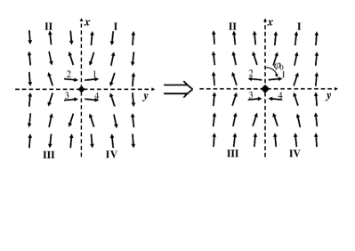
Figure 1: ’Coated’ magnetic polaron before (left figure) and after (right figure) transformation of angles in one sublattice. The magnetic structure is calculated by solving Eqs. (III) at $t/J=50$, $\varkappa=5\times 10^{-3}$. At this values of parameters, $\varphi_{0}=85^{\circ}$.

There is another solution corresponding to the magnetic polaron state with magnetic moment perpendicular to the easy axis: a ’coated’ magnetic polaron. Let us assume again that all spins in the lattice lie in the $xy$ plane, that is, $\theta_{\mathbf{n}}=\pi/2$. It is clear from symmetry that angles $\varphi_{i}\equiv\varphi_{\mathbf{n}_{i}}$ for the local spins inside the magnetic polaron should satisfy the conditions

$$\varphi_{1}=\varphi_{3}=\varphi_{0},\,\,\,\varphi_{2}=\varphi_{4}=-\varphi_{0},$$ (5)

where $0<\varphi_{0}\leq\pi/2$ (see Fig. 1). Minimizing the total energy Eq. (4) with respect to $\varphi_{\mathbf{n}}=\varphi_{n_{x},n_{y}}$, taking into account relation (3) for $E_{\text{el}}$ and the fact that $\Delta\omega=0$ for a planar configuration of spins, we find the following set of nonlinear equations

$$\sum_{{\bm{\Delta}}}\sin(\varphi_{\mathbf{n}+{\bm{\Delta}}}-\varphi_{\mathbf{n}})-\frac{\varkappa}{2}\sin 2\varphi_{\mathbf{n}}=$$

$$=\frac{t}{2J}\sum_{i}\delta_{\mathbf{nn}_{i}}(-1)^{i}\cos\varphi_{i},$$ (6)

where $\varkappa=2K/J$, $\delta_{\mathbf{nm}}$ is the Kronecker symbol, and ${\bm{\Delta}}$ takes values $\{\pm 1,\,0\}$, $\{0,\,\pm 1\}$.

Equations (III) with conditions (5) are solved numerically for the cluster containing $40\times 40$ sites. The further growth of the number of sites in the cluster does not change the obtained results. The initial angle $\varphi_{0}$ is also found. The calculated magnetic structure is shown in Fig. 1. We see from this figure that, in contrast to the ’bare’ ferron, the ’coated’ magnetic polaron produces spin distortions of AFM background outside the region of electron localization. In addition, the ’coated’ magnetic polaron has a magnetization lower than its saturation value ($\varphi_{0}<\pi/2$). Moreover, the ’coat’ has a magnetic moment opposite to that of the core (sites 1– 4 in Fig. 1).

In order to get analytical estimations for the spatial distribution of the spin distortions, we find an approximate solution to Eqs. (III) in the continuum limit. Namely, angles $\varphi_{\mathbf{n}}$ are treated as values of continuous function $\varphi(\mathbf{r})$ at points $\mathbf{r}=\mathbf{n}-\mathbf{n}_{0}$. Assuming that outside the magnetic polaron the following condition is met $|\varphi_{\mathbf{n}+{\bm{\Delta}}}-\varphi_{\mathbf{n}}|\ll 1$, we can expand $\varphi(\mathbf{r}+{\bm{\Delta}})$ in the Taylor series up to the second order in $\Delta$

$$\varphi(\mathbf{r}+{\bm{\Delta}})\approx\varphi({\mathbf{r}})+\Delta^{\alpha}\partial_{\alpha}\varphi({\mathbf{r}})+\frac{1}{2}\Delta^{\alpha}\Delta^{\beta}\partial_{\alpha}\partial_{\beta}\varphi({\mathbf{r}})\,.$$ (7)

Substituting this expansion into Eq. (III), we find that function $\varphi(\mathbf{r})$ outside the magnetic polaron should satisfy the 2D sine-Gordon equation

$$\Delta\varphi-\frac{\varkappa}{2}\sin 2\varphi=0\,.$$ (8)

In the range of parameters under study, $K\ll J$, that is $\varkappa\ll 1$, we can linearize this equation. As a result, we obtain

$$\Delta\varphi-\varkappa\varphi=0\,.$$ (9)

This equation should be solved with the boundary conditions at infinity $\varphi(\mathbf{r})|_{r\to\infty}\!\!\to 0$ and with some boundary conditions at the surface of the magnetic polaron. We model the magnetic polaron by a circle of radius $a=1/\sqrt{2}$ (in the units of lattice constant $d$) and choose the Dirichlet boundary conditions

$$\varphi(\mathbf{r})|_{r=a}=\tilde{\varphi}(\zeta)\,,$$ (10)

where we introduce polar coordinates $(r,\zeta)$ in the $xy$ plane. The function $\tilde{\varphi}(\zeta)$ can be found in the following way. Note, that $\tilde{\varphi}(\zeta)$ should satisfy the symmetry conditions (5) at points $\zeta_{i}=\pi(2i-1)/4$

$$\tilde{\varphi}\left(\zeta_{i}\right)=\varphi_{i}\,,\,\,i=1\dots 4\,.$$ (11)

Since the function $\tilde{\varphi}(\zeta)$ is a periodic one, it can be expanded in the Fourier series

$$\tilde{\varphi}(\zeta)=\sum\limits_{m=0}^{\infty}\left[a_{m}\cos m\zeta+b_{m}\sin m\zeta\right]\,.$$ (12)

In Eq. (12) we neglect the terms with $m>2$ which allows us to keep the minimum number of terms to satisfy the conditions (11). It follows from Eq. (11) that $a_{0}=a_{1}=a_{2}=b_{1}=0$. Finally, we obtain

$$\tilde{\varphi}(\zeta)=\varphi_{0}\sin 2\zeta\,.$$ (13)

Figure 2: Angles $\varphi_{n,n}$ (circles) calculated by solving numerically Eqs. (III) at $t/J=50$, $\varkappa=5\times 10^{-2}$ ($r_{0}\simeq 4.5$). The curve corresponds to the function $\varphi(n-1/2,n-1/2)$, see Eq. (14). The initial angle $\varphi_{0}$ in Eq. (14) is used as a fitting parameter. The range of distances where the quantum fluctuations can play an important role at $S=2$ is shown by the dashed line.

Figure 3: $\varphi(x,y)$ vs $\zeta=\arctan(x/y)$ at $x+y=N$ for $N=3,\,4,\,5,\,7$ from the top to bottom calculated according to Eq. (14) (dashed curves). Points correspond to the numerical calculations of angles $\varphi_{n,N-n+1}$ ($\zeta_{n}=\arctan[(n-1/2)/(N-n+1/2)]$). Parameters of the model are $t/J=50$, $\varkappa=5\times 10^{-2}$.

The solution to Eq. (9) with boundary condition (10) is

$$\varphi(\mathbf{r})=\frac{\varphi_{0}}{K_{2}(a/r_{0})}K_{2}\left(\frac{r}{r_{0}}\right)\sin 2\zeta,\,\,r_{0}=\frac{1}{\sqrt{\varkappa}}\,,$$ (14)

where $K_{2}(x)$ is the Macdonald function. Within the range $|\mathbf{r}|<r_{0}$, $\varphi(\mathbf{r})$ behaves as $a^{2}/r^{2}$, whereas at large distances, it decreases exponentially $\varphi(\mathbf{r})\propto\exp(-r/r_{0})$. The function $\varphi(\mathbf{r})$ at $\zeta=\pi/4$ and the numerical results for $\varphi_{n,n}$ are plotted in Fig. 2. In order to compare the angular dependence of the approximate solution with the numerical results, we plot in Fig. 3 the values of $\varphi(x,y)$ at lines $x+y=N$ depending on the angle $\zeta=\arctan(x/y)$ at different $N$. The values of $\varphi_{n,N-n+1}$ are also shown in this figure. We see from these figures that, except for the small region near the magnetic polaron, the continuous function Eq. (14) is a good interpolation of the function $\varphi_{n_{x},n_{y}}$ at the discrete lattice. Note that at small $r$, the continuum approximation fails because of the large derivatives of $\varphi(\mathbf{r})$. In addition, we cannot neglect the nonlinearity of differential equation (8) in this region.

Figure 4: The energy difference $\Delta E$ between ’coated’ and ’bare’ ferrons vs $\varkappa=2K/J$ calculated at $t/J=50$. Solid curve corresponds to the numerical calculations, whereas dashed curve is calculated using Eq. (16).

Let us calculate now the energy of ’coated’ magnetic polaron, $E_{\text{p}}$, in comparison to the ’bare’ one $E_{\text{p}}^{0}=-2t+16J$. The energy of the system is given by Eq. (4), where $\theta_{\mathbf{n}}=\pi/2$ and $\varphi_{\mathbf{n}}$ is a solution to Eq. (III). In the continuum approximation, we expand $\cos\nu_{\mathbf{nm}}$ and $\cos^{2}\varphi_{\mathbf{n}}$ in the Taylor series up to the second order outside the ferron core. Changing the summation by integration over $\mathbf{r}$, we find for the last two terms in Eq. (4)

$$8J\left(1+\frac{\varkappa}{4}\right)\sin^{2}\varphi_{0}+\frac{J}{2}\!\!\!\int\limits_{|\mathbf{r}|\geq a}\!\!\!d^{2}r\left[({\bm{\nabla}}\varphi)^{2}+\varkappa\varphi^{2}\right]\,.$$ (15)

In Eq.(15), the first term comes from the summation over spins in the core of the magnetic polaron. Substituting solution (14) into Eq. (15) and performing the integration, we find

$$E_{\text{p}}=8J\left(1+\frac{\varkappa}{4}\right)\sin^{2}\varphi_{0}+\frac{J\varphi_{0}^{2}}{2}I(a\sqrt{\varkappa})-2t\sin\varphi_{0}\,,$$ (16)

where

$$I(\rho_{0})=2\pi\left[1+\frac{\rho_{0}K_{1}(\rho_{0})}{2K_{2}(\rho_{0})}\right]\,.$$ (17)

The initial angle $\varphi_{0}$ is found by minimization of energy (16). This value turns out to be slightly different from that found numerically. The dependence of $\Delta E=E_{\text{p}}-E_{\text{p}}^{0}$ on $\varkappa$ is shown in Fig. 4. We see from this figure that $\Delta E<0$ at not too high values of anisotropy constant $K$. So, the magnetic polaron with extended spin distortions can be more favorable than the ’bare’ one. Note also that formula (16) overestimates the energy of the ’coated’ magnetic polaron.

IV Magnetic polaron in 3D lattice

In this section, we calculate the magnetic structure of the ’coated’ magnetic polaron in the 3D case using the approach described above. In the $V\to\infty$ limit, a magnetic polaron includes $8$ sites, that is, $\Psi_{\mathbf{n}}\neq 0$ only for $\mathbf{n}_{1}=\{1,\,1,\,1\}$, $\mathbf{n}_{2}=\{1,\,0,\,1\}$, $\mathbf{n}_{3}=\{0,\,0,\,1\}$, $\mathbf{n}_{4}=\{0,\,1,\,1\}$, $\mathbf{n}_{5}=\{0,\,1,\,0\}$, $\mathbf{n}_{6}=\{1,\,1,\,0\}$, $\mathbf{n}_{7}=\{1,\,0,\,0\}$, $\mathbf{n}_{8}=\{0,\,0,\,0\}$. The electron energy is found then by the diagonalization of the corresponding $8\times 8$ matrix. As in previous section, we assume that all spins in the lattice lie in the $xy$ plane. The symmetry conditions then become

$$\left\{\begin{array}[]{rcl}\varphi_{1}=\varphi_{3}=\varphi_{5}=\varphi_{7}&=&\varphi_{0},\\ \varphi_{2}=\varphi_{4}=\varphi_{6}=\varphi_{8}&=&-\varphi_{0}\,.\end{array}\right.$$ (18)

Minimizing total energy (4) with respect to $\varphi_{\mathbf{n}}$, we get a system of equations similar to Eqs. (III) with the only difference that the factor at the sum in the right-hand side is equal now to $3t/8J$ and ${\bm{\Delta}}$ takes values $\{\pm 1,\,0,\,0\}$, $\{0,\,\pm 1,\,0\}$, and $\{0,\,0,\,\pm 1\}$. We solve this system of equations numerically for the cluster with $30\times 30\times 30$ sites.

In the continuum approximation, the magnetic structure is found in the same manner as in the 2D case. We consider a spherical magnetic polaron of radius $a=\sqrt{3}/2$. The function $\varphi(\mathbf{r})$ satisfies Eq. (9) with the boundary conditions at $|\mathbf{r}|=a$

$$\varphi(\mathbf{r})|_{r=a}=\tilde{\varphi}(\vartheta,\zeta)\,,$$ (19)

where $r$, $\vartheta$, and $\zeta$ are spherical coordinates and the function $\tilde{\varphi}(\vartheta,\zeta)$ should satisfy the symmetry conditions (18) at angles $\vartheta_{i}$, $\zeta_{i}$ corresponding to the directions of $\mathbf{n}_{i}-\mathbf{n}_{0}$ ($i=1\dots 8$). Expanding $\tilde{\varphi}(\vartheta,\zeta)$ in series of spherical functions $\text{Y}_{lm}(\vartheta,\zeta)$ and retaining only the terms with the smallest $l$, one finds

$$\tilde{\varphi}(\vartheta,\zeta) = \varphi_{0}\sqrt{\frac{36\pi}{35}}\left[\text{Y}_{3,+2}(\vartheta,\zeta)-\text{Y}_{3,-2}(\vartheta,\zeta)\right]$$ (20)

$$= \varphi_{0}\sqrt{\frac{27}{2}}\sin^{2}\vartheta\cos\vartheta\sin 2\zeta\,.$$

The solution to Eq. (9) with the boundary conditions (19) is

$$\varphi(x,y,z)=\varphi_{0}\frac{R_{3}(r/r_{0})}{R_{3}(a/r_{0})}\frac{3\sqrt{3}\,xyz}{r^{3}}\,,$$ (21)

where again $r_{0}=1/\sqrt{\varkappa}$, and

$$R_{3}(\rho)=\left(1+\rho+\frac{2\rho^{2}}{5}+\frac{\rho^{3}}{15}\right)\displaystyle\frac{\text{e}^{-\rho}}{\rho^{4}}\,.$$ (22)

Figure 5: The dependence of $\varphi(\mathbf{r})$ on the distance $r$ in the direction $\{1,\,1,\,1\}$ calculated according to Eq. (21) (solid and dashed curve). Circles represent the numerical results for $\varphi_{n,n,n}$ at $t/J=100$, $\varkappa=5\times 10^{-2}$. The initial angle $\varphi_{0}$ in Eq. (21) is used as a fitting parameter. The range of distances where the quantum fluctuations can play an important role at $S=2$ is shown by the dashed line. In the inset, the dependence of $\Delta E$ on $\varkappa$ is shown. The energy difference $\Delta E$ is calculated numerically at $t/J=100$.

It follows from Eqs. (21) and (22) that $\varphi(\mathbf{r})$ decreases at $r<r_{0}$ as $a^{4}/r^{4}$. At distances $r$ exceeding characteristic radius $r_{0}$, the spin distortions decay exponentially, $\varphi(\mathbf{r})\propto\exp(-r/r_{0})$ as in the 2D case. The dependence of $\varphi(\mathbf{r})$ on distance $r$ in the $\mathbf{n}_{1}=\{1,\,1,\,1\}$ direction is shown in Fig. 5. The numerical results for $\varphi_{n,n,n}$ are also presented in this figure.

The energy of the magnetic polaron, $E_{\text{p}}$, is found in the same way as in the previous section. Note that in the 3D case, the energy of a ’bare’ magnetic polaron is $E_{\text{p}}^{0}=-3t+48J$. The dependence of $\Delta E=E_{\text{p}}-E_{\text{p}}^{0}$ on $\varkappa$ is shown in the inset to Fig. 5. We see that in the 3D case, the situation is similar to that considered in the previous section. At not too high anisotropy constant, the ’coated’ magnetic polaron is favorable in energy in comparison to the ’bare’ one.

Note, however, that the two-sublattice AFM state considered here is not eigenstate of the system, and quantum fluctuations play an important role. Indeed, the fluctuation magnitude is about $\delta S/S=0.078/S$ for the isotropic 3D Heisenberg model Kittel . This value becomes of the order of the angle $\phi$ at $r=2$ (second coordination sphere). However, we consider the situation with uniaxial anisotropy, which drastically reduces quantum fluctuations stabilizing the two-sublattice AFM state. For example, for manganites, the characteristic value of the anisotropy parameter $K=0.05J$ (see Ref. Nikiforov, ). At such anisotropy, the fluctuation magnitude decreases by about 30%. This means that we can use our results up to $r=3$. At the concentrations of the impurities higher than 1% the distance between impurities is less than 6 lattice constants and the behavior of the distortions at $r>3$ is not of real physical importance. The similar arguments are valid also for the 2D case. Here, we can find that $\delta S/S=0.092/S$ at $K=0.05J$ (note that the magnetic anisotropy stabilizes the long-range magnetic order in the 2D Heisenberg model). In 2D, the distortions of AFM order decay slower than in the 3D case. Thus, the quantum fluctuations become comparable to the angle $\phi$ at $r\simeq 4$. The range of distances where the quantum fluctuations can play an important role at $S=2$ is shown by the dashed line in Figs. 2 and 5.

V Conclusions

We studied the structure of bound magnetic polarons in 2D and 3D antiferromagnets doped by nonmagnetic donor impurities. The doping concentration was assumed to be small enough, and the system is far from the insulator-metal transition. It was also assumed that the conduction electron is bound by electrostatic potential of impurity with the localization length $a$ close to the lattice constant $d$. We found two possible types of magnetic polarons, ’bare’ and ’coated’. At not too high constant of magnetic anisotropy $K\ll J$, the ’coated’ polarons correspond to a lower energy. Such a ’coated’ ferron consists of a ferromagnetic core of the size $a$ and extended spin distortions of the AFM matrix around it. The characteristic radius of distortions is $r_{0}=d\sqrt{J/2K}$. Within the $a<r<r_{0}$ range, these spin distortions behave as $a^{2}/r^{2}$ in the 2D case and as $a^{4}/r^{4}$ in the 3D case. At larger distances, they decay exponentially as $\exp(-r/r_{0})$. Note that in real systems, the constant of magnetic anisotropy $K$ is small enough in comparison to exchange integral $J$ and the characteristic radius $r_{0}$ can be rather large.

The calculations have been performed in the case of zero temperature $T=0$. At finite temperatures, the regular picture of spin distortions could be, in principle, destroyed, owing to the spin-wave excitations. However, in the case of uniaxial anisotropy, the spin-wave spectrum has a gap of the order of $\sqrt{2KJ}$. So, the characteristic temperature, below which our results (in particular, those presented in Figs. 2 and 5) are applicable, is of the same order. For example, in manganites, a typical value of this temperature is 5 K.

Note that in the 1D case, the ’coated’ ferron was found to be a metastable object Fer1D in contrast to the 2D and 3D cases considered here. The cause of such a difference is the following. In the 1D case, the ’bare’ magnetic polaron has zero surface energy since it does not disturb the AFM ordering at its border. For $D>1$, the surface energy is nonzero due to the geometry of the problem. For the ’coated’ magnetic polaron, the surface energy is nonzero at any dimension. However, the extended ’coat’ reduces its value.

Our results were obtained in the limit of strong electron-impurity coupling, $V\to\infty$. In this case, the wave function $\Psi_{\mathbf{n}}$ of the conduction electron is nonzero only at the sites nearest to the impurity, and one can calculate the electron energy $E_{\text{el}}$ exactly. At finite $V$, the wave function extends over larger distances and one should calculate the magnetic structure simultaneously with $\Psi_{\mathbf{n}}$. Note, that even at $V=0$, the magnetic polaron is a stable object in a wide range of parameters of the model. This is the so called self-trapped magnetic polaron, which exists due to trapping of a charge carrier in the potential well of ferromagnetically oriented local spins Nag67 . The radius of such a polaron was estimated as $a\sim d(t/J)^{1/5}$ and at large $t/J$ it can be of the order of several lattice constants Kak ; Kkm .

Let us find the range of validity for the assumption $V\to\infty$ used in this paper. For this purpose, we rewrite the electron energy $E_{\text{el}}$ in terms of the wave function. Performing the transformation of angles described in Section III, and using the substitution $\Psi_{\mathbf{n}}=\text{e}^{i\varphi_{\mathbf{n}}/2}\psi_{\mathbf{n}}$, we can write at $\theta_{\mathbf{n}}=\pi/2$

$$E_{\text{el}}=t\sum_{\langle\mathbf{nm}\rangle}\sin\left(\frac{\varphi_{\mathbf{n}}-\varphi_{\mathbf{m}}}{2}\right)\text{Im}\left(\psi_{\mathbf{n}}\psi_{\mathbf{m}}^{*}\right)-V\sum_{\mathbf{n}}\frac{\left|\psi_{\mathbf{n}}\right|^{2}}{|\mathbf{n-n}_{0}|}.$$

Minimizing the total energy with respect to angles $\varphi_{\mathbf{n}}$, we obtain the set of equations similar to Eqs. (III) with the right-hand side in the form

$$\frac{t}{2J}\sum_{\bm{\Delta}}\cos\left(\frac{\varphi_{\mathbf{n}+\bm{\Delta}}-\varphi_{\mathbf{n}}}{2}\right)\text{Im}\left(\psi_{\mathbf{n}}\psi_{\mathbf{n}+\bm{\Delta}}^{*}\right)\,.$$ (23)

In the limit of strong electron-impurity coupling, we can assume that the wave function is hydrogen-like, that is, $|\psi_{\mathbf{n}}|\approx N_{\text{p}}^{-1/2}\exp[-(d|\mathbf{n-n}_{0}|-a)/a_{B}^{*}]$, where $N_{\text{p}}$ is the number of sites inside the magnetic polaron and $a_{B}^{*}$ is the effective Bohr radius. The latter one can be estimated as $a_{B}^{*}=\hbar^{2}\epsilon/m^{*}e^{2}$, where $\epsilon$ is the permittivity, and $m^{*}$ is the effective electron mass, which can be found from the relation $\hbar^{2}/2m^{*}=td^{2}$. Taking into account these estimations, we find that one can neglect the right-hand side (23) in Eq. (III) for $\mathbf{n}\neq\mathbf{n}_{i}$ if

$$\frac{t}{2JN_{\text{p}}}\text{e}^{-V/2t}\ll 1\,.$$

In the 3D case, we have $N_{\text{p}}=8$, and the approximation $V\to\infty$ is valid for $V=e^{2}/\epsilon d$ down to $V_{c}=2t\ln(t/16J)$. For realistic values of parameters $V$ is usually of the order of $V_{c}$. So, it is of interest to perform a more detailed analysis of the problem at finite values of $V$ similar to that discussed in Ref. Ivan2, for the 1D case. Nevertheless, we hope that our results concerning the extended spin distortions are valid also at $V<V_{c}$, and, consequently, for magnetic polarons with larger sizes $a$. Indeed, in the continuum approximation, the dependence of the magnetic structure on $a$ is not so important. Moreover, the energy of the magnetic polaron $E_{\text{p}}$ formally depends on $a$ only through the term $J\varphi_{0}^{2}I(a\sqrt{\varkappa})/2\sim J$ coming from the spatial integration (see Eq. (16)). Since $\varkappa\ll 1$, the energy difference $\Delta E$ is negative up to $a\sim r_{0}\gg d$.

In our paper, we studied the isolated ferrons. However, as it was already mentioned above, the substantial overlap of the extended distortions can arise even at very low doping (about 1%). As a result, the magnetic moments of the ferrons could be ordered. In particular, according to Ref. Nag01, , in such a situation, there can exist a long-range ferromagnetic order with the magnetic moment far from the saturation value.

References

- (1) E. Dagotto, Nanoscale Phase Separation and Colossal Magnetoresistance: The Physics of Manganites and Related Compounds (Springer-Verlag, Berlin, 2003).
- (2) E. Dagotto, Science 309, 257 (2005); New J. Phys. 7, 67 (2005).
- (3) P.L. Kuhns, M.J.R. Hoch, W.G. Moulton, A.P. Reyes, J. Wu, and C. Leighton, Phys. Rev. Lett. 91, 127202 (2003).
- (4) G. Blumberg, M.V. Klein, and S.-W. Cheong, Phys. Rev. Lett. 80, 564 (1998); R. Lemanski, J.K. Freericks, and G. Banach, Phys. Rev. Lett. 89, 196403 (2002).
- (5) H. Seo, C. Hotta, and H. Fukuyama, Chem. Rev. 104, 5005 (2004).
- (6) A.H. Castro Neto and B.A. Jones, Phys. Rev. B62, 14975 (2000); P. Chandra, P. Coleman, J.A. Mydosh, and V. Tripathi, Nature (London) 417, 831 (2002).
- (7) L.N. Bulaevskii, E.L. Nagaev, and D.I. Khomskii, Zh. Eksp. Teor. Fiz. 54, 1562 (1968) [Sov. Phys. JETP 27, 836 (1968)].
- (8) L.V. Keldysh, phys. stat. sol. (a) 164, 3 (1997).
- (9) J. Zaanen and O. Gunnarsson, Phys. Rev. B 40, 7391 (1989).
- (10) C. Castellani, C. Di Castro, and M. Grilli, Phys. Rev. Lett. 75, 4650 (1995).
- (11) E.L. Nagaev, Usp. Fiz. Nauk 165, 529 (1995) [Physics-Uspekhi 38, 497 (1995)].
- (12) V.J. Emery, S.A. Kivelson, and H.Q. Lin, Phys. Rev. Lett. 64, 475 (1990).
- (13) A. Kampf and J.R. Schrieffer, Phys. Rev. B41, 6399 (1990).
- (14) E.L. Nagaev, Pis’ma Zh. Eksp. Teor. Fiz. 6, 484 (1967) [JETP Lett. 6, 18 (1967)].
- (15) T. Kasuya, A. Yanase, and T. Takeda, Solid State Commun. 8, 1543, 1551 (1970).
- (16) P.G. de Gennes, Phys. Rev. 118, 141 (1960).
- (17) E.L. Nagaev, Pis’ma Zh. Eksp. Teor. Fiz. 74, 472 (2001) [JETP Lett. 74, 431 (2001)].
- (18) J. Castro, I. González, and D. Baldomir, Eur. Phys. J. B 39, 447 (2004).
- (19) I. González, J. Castro, D. Baldomir, A.O. Sboychakov, A.L. Rakhmanov, and K.I. Kugel, Phys. Rev. B69, 224409 (2004).
- (20) M.Yu. Kagan, A.V. Klaptsov, I.V. Brodsky, K.I. Kugel, A.O. Sboychakov, and A.L. Rakhmanov, J. Phys. A 36, 9155 (2003).
- (21) M. Hennion, F. Moussa, G. Biotteau, J. Rodríguez-Carvajal, L. Pinsard, and A. Revcolevschi, Phys. Rev. Lett. 81, 1957 (1998).
- (22) M. Hennion, F. Moussa, G. Biotteau, J. Rodríguez-Carvajal, L. Pinsard, and A. Revcolevschi, Phys. Rev. B61, 9513 (2000).
- (23) M. Hennion and F. Moussa, New J. Phys. 7, 84 (2005).
- (24) M. Hennion, F. Moussa, P. Lehouelleur, F. Wang, A. Ivanov, Ya.M. Mukovskii, and D. Shulyatev, Phys. Rev. Lett. 94, 057006 (2005).
- (25) M.V. Berry, Proc. Roy. Soc. London A 392, 45 (1984).
- (26) E. Müller-Hartmann and E. Dagotto, Phys. Rev. B54, R6819 (1996).
- (27) C. Kittel, Quantum Theory of Solids (Wiley, New York, 1963).
- (28) L.E. Gontchar, A.E. Nikiforov, and S.E. Popov, J. Magn. Magn. Mater. 223, 175 (2001).
- (29) M.Yu. Kagan and K.I. Kugel, Usp. Fiz. Nauk 171, 577 (2001) [Physics - Uspekhi 44, 553 (2001)].
- (30) M.Yu. Kagan, D.I. Khomskii, and M.V. Mostovoy, Eur. Phys. J. B, 12 217 (1999).
- (31) A.O. Sboychakov, A.L. Rakhmanov, K.I. Kugel, I. González, J. Castro, and D. Baldomir, Phys. Rev. B72, 014438 (2005).
- (32) E.L. Nagaev, Pis’ma Zh. Eksp. Teor. Fiz. 74 472 (2001) [JETP Lett. 74, 431 (2001)].