Intervalley scattering, long-range disorder, and effective time reversal symmetry breaking in graphene.

Abstract

We discuss the effect of certain types of static disorder, like that induced by curvature or topological defects, on the quantum correction to the conductivity in graphene. We find that when the intervalley scattering time is long or comparable to $\tau_{\phi}$, these defects can induce an effective time reversal symmetry breaking of the hamiltonian associated to each one of the two valleys in graphene. The phenomenon suppresses the magnitude of the quantum correction to the conductivity and may result in the complete absence of a low field magnetoresistance, as recently found experimentally. Our work shows that a quantitative description of weak localization in graphene must include the analysis of new regimes, not present in conventional two dimensional electron gases.

Introduction. Graphene provides a two-dimensional electron system that is distinctly different from the two-dimensional electron gases (2DEGs) hosted in common semiconducting heterostrutures. The low energy electronic states of graphene can be described by two sets of two-dimensional spinors associated to two independent points at the corner of the Brillouin zone ($K$ and $K^{\prime}$). In the absence of short range potentials the states associated to the different points are not coupled and, in the long wavelength limit, they satisfy the two dimensional Dirac equation. Theoretical calculations based on these assumptionsPeres et al. (2006) reproduce the unconventional quantization of the quantum Hall conductance observed experimentally Novoselov et al. (2005); Zhang et al. (2005) (see alsoKopelevich et al. (2003)). It is expected that, beside the quantum Hall effect, other phenomena should manifest unusual characteristics as compared to more conventional 2DEGs.

It appears that one of these phenomena is the weak-localization correction to the conductivityAltshuler et al. (1980); Larkin and Khmel’nitskii (1982); Bergman (1984); Khmel’nitskii (1984). In the presence of time-reversal symmetry, the suppression of weak-localization at low magnetic fields produces a negative magnetoresistance, ubiquitous in metallic conductors. The magnitude of the weak-localization correction is of the order of $e^{2}/h$ and it is determined by two characteristic time scales: the phase coherence time $\tau_{\phi}$ and the elastic scattering time $\tau$. In the graphene samples that exhibit very clear QHE, however, no low-field magnetoresistance is observed. In these samples, nevertheless, the observation of high-order quantum Hall plateau indicates that phase coherent propagation of electrons occurs at least on a distance of several hundreds nanometers, which corresponds to the estimated elastic mean-free path, so that a magnetoresistance originating from the suppression of weak-localization is expected.

It has been realized by Suzuura and AndoSuzuura and Ando (2002) that the quantum correction to the conductivity in graphene can differ from what is observed in conventional 2DEGs (see alsoKhveshchenko (2006)). This is due to the pseudo-spin associated to the solutions of the Dirac equation, that in conjunction with the nature of elastic scattering in graphene may change the sign of the localization correction, and turn weak-localization into weak-antilocalization (even in the absence of spin-orbit interaction). The phenomenon crucially depends on the inter-valley scattering time $\tau_{\rm iv}$, i.e. the characteristic times that it takes for a charge carrier to be scattered from one to the other $K$-point in graphene. Specifically, if $\tau_{\rm iv}\gg\tau_{\phi}$ weak antilocalization is expected, resulting in a positive magnetoresistance at low field; if $\tau_{\rm iv}\ll\tau_{\phi}$, conventional weak localization should be observed. Even though these conclusions are at odds with experimental findings, they are important as they clearly illustrate the relevance of inter-valley scattering.

Here, we show that not only weak localization and antilocalization can appear in graphene depending on the nature of elastic scattering, but also that the quantum correction to the conductivity can be entirely suppressed due to time-independent potential slowly varying in space. These static potentials can result in the effective breaking of time reversal symmetry of electronic states around each $K$-point when $\tau_{iv}>\tau_{\phi}$. They originate from defects that are realistically present in graphene, such as long-range distortions induced by topological lattice defects (disclinations and dislocations), non-planarity of the graphene layers, and slowly varying random electrostatic potentials that break the symmetry between the two sublattices of graphene. We estimate the effect of each one of these defects in terms of a characteristic time, which acts as a cut off for the time-reversed trajectories of electrons responsible for weak-localization phenomena. If the characteristic time associated to one of these mechanisms is much shorter than $\tau_{\phi}$, weak-localization is largely suppressed. This explains the absence of weak-localization in the first magneto-transport experiments in graphene.

We emphasize that the potentials that we consider, being static, do not actually break time reversal symmetry in graphene. However, in the presence of these potentials, time reversal symmetry connects electronic states associated to the two different $K$-points. If the electron dynamics is such that electrons cannot be transferred from one to the other $K$-point within their phase coherence time (i.e., if $\tau_{iv}>\tau_{\phi}$), the contribution to interference due to time-reversed trajectories (responsible for weak-localization) is suppressednot (a).

The model. We use the continuum approximation to the band structure near the $K$ and $K^{\prime}$ points of the Brillouin Zone of graphene. The wavefunctions can be expressed as a two component spinor, $[\Psi_{A,K,\uparrow}({\bf\vec{r}}),\Psi_{B,K,\uparrow}({\bf\vec{r}})]$, where $A$ and $B$ stand for the two sublattices of the honeycomb structure. Other spinors can be defined for the $K^{\prime}$ point and the down spin orientation. The curvature of the graphene sheet can be included by generalizing the ordinary derivative operator to the covariant derivativeGonzález et al. (1992, 1993), following the standard procedure used for spinor fieldsBirrell and Davies (1982). These effects are described below by the spin connection operator $\hat{\bf\Sigma}_{\rm curv}$ which breaks the effective time reversal symmetry around each $K$ point. Similarly, certain topological lattice defects imply the existence of rings with an odd number of Carbon atoms. A dislocation has a pentagon at its core, and a dislocation requires a pentagon-heptagon pair. An odd numbered ring of Carbon atoms implies that the two sublattices are interchanged when traversing a path which encloses it. This needs to be taken into account in the continuum description, irrespective of the smoothness of the induced distortion. It can be described by a non Abelian gauge potential $\hat{\bf\Sigma}_{\rm def}$ González et al. (1992, 1993). It has been shown that its inclusion allows for an accurate description of the electronic spectrum in curved graphene sheets, such as fullerenesGonzález et al. (1992, 1993), or graphitic conesLammert and Crespi (2000). Note that this gauge field interchanges the two sublattices and the $K$ and $K^{\prime}$ points. This fact, however, does not prevent the description of the system in terms of two sets of spinorial wavefunctions which obbey equivalent Dirac equations. In fact, using the transformation:

$$\tilde{\Psi}_{A{\cal K}{\bf\vec{k}}s}({\bf\vec{r}}) = \Psi_{AK{\bf\vec{k}}s}({\bf\vec{r}})+i\Psi_{BK^{\prime}{\bf\vec{k}}s}({\bf\vec{r}})$$

$$\tilde{\Psi}_{B{\cal K^{\prime}}{\bf\vec{k}}s}({\bf\vec{r}}) = \Psi_{BK^{\prime}{\bf\vec{k}}s}({\bf\vec{r}})-i\Psi_{AK{\bf\vec{k}}s}({\bf\vec{r}})$$ (1)

the model can be reduced to two independent hamiltonians:

$${\cal H}_{{\cal K},s} \equiv \left(\begin{array}[]{cc}\Delta({\bf\vec{r}})&v_{\rm F}(i\partial_{x}+\partial_{y})+{\hat{\bf A}}_{x}+i{\hat{\bf A}}_{y}+\hat{\bf\Sigma}_{\rm curv}+\hat{\bf\Sigma}_{\rm def}\\ v_{\rm F}(i\partial_{x}-\partial_{y})+{\hat{\bf A}}_{x}-i{\hat{\bf A}}_{y}+\hat{\bf\Sigma}_{\rm curv}+\hat{\bf\Sigma}_{\rm def}&-\Delta({\bf\vec{r}})\end{array}\right)$$ (4)

$${\cal H}_{{\cal K^{\prime}},s} \equiv \left(\begin{array}[]{cc}\Delta({\bf\vec{r}})&v_{\rm F}(i\partial_{x}-\partial_{y})+{\hat{\bf A}}_{x}-i{\hat{\bf A}}_{y}+\hat{\bf\Sigma}_{\rm curv}-\hat{\bf\Sigma}_{\rm def}\\ v_{\rm F}(i\partial_{x}+\partial_{y})+{\hat{\bf A}}_{x}+i{\hat{\bf A}}_{y}+\hat{\bf\Sigma}_{\rm curv}-\hat{\bf\Sigma}_{\rm def}&-\Delta({\bf\vec{r}})\end{array}\right)$$ (7)

where $\hat{\bf A}$ is the ordinary vector potential. $\Delta({\bf\vec{r}})=V_{\rm A}({\bf\vec{r}})-V_{\rm B}({\bf\vec{r}})$ measures the difference of the electrostatic potential in the two sublattices and originates from the environment around the graphene layer (e.g., charges located at random position in the substrate supporting graphene).

A description of quantum interference in terms states associated to two decoupled K-points separately is correct if $\tau_{\rm iv}\gg\tau_{\phi}$. In this regime, the defects described by three terms $\hat{\bf\Sigma}_{\rm def},\hat{\bf\Sigma}_{\rm curv}$ and $\Delta({\bf\vec{r}})$ break the effective time reversal symmetry around the ${\it K}$ and ${\it K^{\prime}}$ points, which can be written as the complex conjugation operator times $\sigma_{y}$McCann and Fal’ko (2004). We will treat separately the effect of the different defects by analyzing the dynamical phase that quasi-classical trajectories in real space acquire in their presence. We will confine ourselves to the qualitative analysis of this problem, but we note that a formal description of weak -(anti)localization in terms of quasi-classical trajectories Larkin and Khmel’nitskii (1982); Khmel’nitskii (1984); Bergman (1984)can be made equivalent to diagrammatic approachesChakravarty and Schmid (1986).

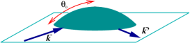
Figure 1: Geometry of the scattering process analyzed in the text. An impurity potential is placed at the center of a spherical bump in a flat sheet.

Curvature effects. Scattering is modified in a curved surface. We analyze the geometry sketched in Fig.[1]. An incoming plane wave moves into a spherical cap parametrized by the angle $\theta$. The wave is scattered by a defect within the bump. We place the defect at the center of the region, in order to simplify the calculation. In flat space, the incoming and outgoing waves can be written as:

$$\begin{array}[]{lr}\Psi_{\bf\vec{k}}\equiv\left(\begin{array}[]{c}1\\ e^{i\phi_{\bf\vec{k}}}\end{array}\right)e^{i{\bf\vec{k}}{\bf\vec{r}}}&\Psi_{\bf\vec{k}^{\prime}}\equiv\left(\begin{array}[]{c}1\\ e^{i\phi_{\bf\vec{k}^{\prime}}}\end{array}\right)e^{i{\bf\vec{k}^{\prime}}{\bf\vec{r}}}\end{array}$$ (8)

where $\phi_{\bf\vec{k}}$ determines the direction of ${\bf\vec{k}}$. The scattering amplitude due to a local potential, $\hat{V}\equiv V\delta({\bf\vec{r}})$ is $A=\langle{\bf\vec{k}}|\hat{V}|{\bf\vec{k}^{\prime}}\rangle\propto V[1+\cos(\phi_{\bf\vec{k}}-\phi_{\bf\vec{k}^{\prime}})]$.

We calculate the scattering amplitude in the geometry shown in Fig.[1] by matching the plane waves in eq.(8) to solutions inside the spherical cap. The wavefunctions can be computed analytically for energies $\epsilon_{l}=v_{\rm F}/R\sqrt{{\bf l}({\bf l}+1)-2}$González et al. (1992). The quasiclassical limit corresponds to ${\bf l}\gg 1$. The main difference between the solutions inside the cap and those in a plane, eq.(8), is that the values of the modulii of the two components of the Dirac spinors are not equal. Because of the radial symmetry of the problem, we only need the solutions inside the cap with $m=0$. The relevant solutions, for a given valley, can be written as:

$$\begin{array}[]{lr}\Psi_{1}\equiv\left(\begin{array}[]{c}\psi_{A}^{1}(\theta)\\ \psi_{B}^{1}(\theta)e^{-i\phi}\end{array}\right)&\Psi_{2}\equiv\left(\begin{array}[]{c}\psi_{A}^{2}(\theta)e^{i\phi}\\ \psi_{B}^{2}(\theta)\end{array}\right)\end{array}$$ (9)

Matching these solutions to those in eq.(8) outside the cap, the scattering amplitude can be written as:

$$A\propto V[|{\psi_{A}^{1}}(\theta_{0})^{2}+{\psi_{B}^{2}}(\theta_{0})^{2}+2{\psi_{A}^{1}}(\theta_{0}){\psi_{B}^{2}}(\theta_{0})\cos(\phi_{\bf\vec{k}}-\phi_{\bf\vec{k}^{\prime}})]$$ (10)

where $\theta_{0}$ is the angle which defines the shape of the cap. The deviation from scattering in a plane is determined by the difference ${\psi_{A}^{1}}(\theta_{0})-{\psi_{B}^{2}}(\theta_{0})$, which is maximum when ${\psi_{A}^{1}}(\theta_{0}),{\psi_{B}^{2}}(\theta_{0})\approx 0$, as shown in Fig.[2].

The first zeros of the functions ${\psi_{A}^{1}}(\theta_{0}),{\psi_{B}^{2}}(\theta_{0})\approx 0$ lie at $\theta_{0}\sim{\bf l}^{-1}$. Hence, we expect deviations from antilocalization for Fermi energies such that $\theta_{0}\sim\epsilon_{\rm F}R/v_{\rm F}$, that is, $k_{\rm F}R\sim 1$. In a sample with height fluctuations of order $h$ oner a length $l$, we have $R^{-1}\sim h^{2}/l$, so that antilocalization effects will be suppressed for $(k_{\rm F}h^{2})/l\sim 1$.

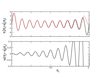
Figure 2: Wavefunctions within the spherical cap shown in Fig.[1] for ${\cal l}=20$. These two solutions, in flat space, are related by the effective time reversal symmetry defined in each valley.

Gauge field induced by lattice defects. As mentioned above, a local rotation of the axes leads to the existence of a gauge field, $\hat{\bf\Sigma}_{\rm def}$. In terms of the lattice strain, $u_{x}({\bf r}),u_{y}({\bf r})$, this rotation is given byGonzález et al. (2001):

$$\theta({\bf r})\approx\frac{\partial_{y}u_{x}-\partial_{x}u_{y}}{2}$$ (11)

and $\hat{\bf\Sigma}_{\rm def}$ in eq.(7) becomes:

$$\hat{\bf\Sigma}_{\rm def}\equiv\frac{1}{2}\nabla\theta({\bf r})$$ (12)

We consider first the effect of gauge field induced by a finite distribution of dislocations, with random Burgess vectors ${\bf b}_{i}$, and average distance $d$, on a quasiparticle moving around a closed loop of length $l$.

At sufficiently long distances from an edge dislocation with Burgess vector ${\bf\vec{b}}$, eq.(11) gives $\theta({\bf r})\propto{\bf\vec{b}}{\bf\vec{r}}/|{\bf r}|^{2}$. The local rotations average to zero when the loop encloses completely the dislocations. A finite contribution is obtained from the dislocations whose core is near the trajectory of the particle. The quasi-classical width of the trajectory of the particle is of order $k_{\rm F}^{-1}$, where $k_{\rm F}$ is the Fermi wavevector. Hence, the number of dislocations which contribute to change the phase around the loop is of order $(k_{\rm F}^{-1}d)/l^{2}$, where $l$ is the length of the loop and $d$ is the average distance between dislocations.

To estimate the effect of the rotation on the phase of the trajectories traversing the loop, we assume that the Burgess vector of the dislocations is distributed randomly. Using the central limit theorem, we find that the rotation associated to the loop becomes non negligible when $[(k_{\rm F}^{-1}d)/l^{2}]^{2}\gg 1$. This rotation leads to a phase of order $\pi$, which dephases randomly trajectories traversed clock- and anticlockwise, which suppresses the quantum interference correction to the conductivity. From the above inequality, the time scale at which these effects are relevant is:

$$\tau_{\rm gauge}^{-1}\sim\frac{v_{\rm F}}{\sqrt{k_{\rm F}^{-1}d}}$$ (13)

Potential gradients. The potential $\Delta({\bf\vec{r}})$ in eq.(7) represents the difference in potentials at the two sites of the unit cell. Physically, this potential originates from charges located in the substrate supporting the graphene layernot (b). An asymmetry between the two sublattices arises from slowly varying potentials, that can be written as the sum of a smooth term which is the same within each unit cell, and a small contribution which breaks the equivalence of the two sites in the unit cell. The second part can be written as $\Delta({\bf\vec{r}})\approx{\bf\vec{c}}\nabla V({\bf\vec{r}})$, We assume this potential to be slowly varying, so that:

$$V({\bf\vec{q}})\approx\left\{\begin{array}[]{lr}V_{0}&|{\bf\vec{q}}|\ll q_{c}\\ 0&|{\bf\vec{q}}|\gg q_{c}\end{array}\right.$$ (14)

where $q_{c}$ is a momentum cutoff such that $q_{c}\ll a^{-1}$, where $a$ is the lattice constant. We are interested in momentum transfers $|{\bf\vec{q}}|\sim k_{\rm F}$, where $k_{\rm F}\ll a^{-1}$ for typical dopings. Eq.(14) implies that:

$$\Delta({\bf\vec{q}})\approx\left\{\begin{array}[]{lr}{\bf\vec{q}}{\bf\vec{c}}V_{0}&|{\bf\vec{q}}|\ll q_{c}\\ 0&|{\bf\vec{q}}|\gg q_{c}\end{array}\right.$$ (15)

The elastic scattering time can be obtained from $V_{\rm disorder}$ using Fermi’s golden rule:

$$\tau_{\rm elastic}^{-1}\approx\frac{V_{0}^{2}\nu(\epsilon_{\rm F})}{a^{2}}$$ (16)

where $\nu(\epsilon_{\rm F})=|\epsilon_{\rm F}|/(\pi v_{\rm F}^{2})$ is the density of states at the Fermi energy.

The potential $\Delta({\bf\vec{r}})$ breaks the effective time reversal symmetry around each $K$ point. We can estimate the inverse time at which this operator induces a significant change in the wavefuction of the spinor applying again Fermi’s golden rule to the symmetry breaking potential:

$$\tau_{\rm grad}^{-1}\approx\frac{V_{0}^{2}\nu(\epsilon_{\rm F})}{a^{2}}|{\bf\vec{c}}|^{2}k_{\rm F}^{2}\sim\tau_{\rm elastic}^{-1}n_{\rm elec}$$ (17)

where $n_{\rm elec}\sim(k_{\rm F}a)^{2}$ is the number of carriers per unit cell (note that the effect can be larger close to the sample edges where the disorder is also larger). In typical experiments, $n_{\rm el}\sim 10^{-4}-10^{-2}$. Thus, there exists a range of energies or temperatures, $\tau_{\rm grad}^{-1}\lesssim T\lesssim\tau_{\rm el}^{-1},\tau^{-1}_{\phi}\ll T$, where the effective time reversal symmetry around each ${\it K}$ is not broken by $\Delta({\bf\vec{r}})$.

Conclusions. Our analysis illustrates that the behavior of the quantum correction to the conductivity in graphene is much richer than what was anticipated in the work of Suzuura and Ando Suzuura and Ando (2002). We conclude that the inter-valley scattering time $\tau_{iv}$ and the phase coherence time $\tau_{\phi}$ are not the only important time scales. An additional time scale describing the effective time reversal symmetry breaking is present, which can cause a complete suppression of weak (anti)localization. This time scale depends on specific defects present in the graphene samples, which leads to the prediction that large differences in the quantum correction to the conductivity measured on different samples should be expected. This is striking, since in all metallic conductors studied in the past weak (antilocalization manifests as a robust and very reproducible phenomenon.

Furthermore, the physical understanding provided by our analysis, which does not rely on any detailed assumption, enables us to draw additional conclusions. For instance, we expect that it will be easier to observe weak-localization in narrow graphene samples, since scattering at the edges couple states at the two different K-points. We also expect that an effective time reversal symmetry breaking similar to the one discussed here should occur more in general, in systems with two or more degenerate valleys with topological defects similar to those considered here. This is the case, for instance, for a graphene bilayerMcCann and Fal’ko (2006); Novoselov et al. (2006). Note, however, that contrary to individual graphene layers, in graphene bilayers the relative phases of the two components in the spinor of the momentum eigenfunctions are twice those in graphene. Therefore, in sufficiently clean samples (where defects are not sufficient to induce an effective time reversal symmetry breaking) the usual negative magnetoresistance is expected, and there should be no weak antilocalization à la Suzuura-Ando.

We gratefully acknowledge very useful discussions with A. Geim, K. Novoselov, P. Kim, B. Trauzettel, A. Castro Neto, N. M. R. Peres, M. Katsnelson, L. Vandersypen, H. Heersche, and P. Jarillo-Herrero. F. G. acknowledges funding from MEC (Spain) through grant FIS2005-05478-C02-01 .

Note added. Since this work was posted, three related works have appearedMorozov et al. (2006); McCann et al. (2006); Nomura and MacDonald (2006) dealing with the same topic. Ref.Morozov et al. (2006) presents experimental results consistent with our work, as well as a theoretical explanation along similar lines. The analysis of weak localization effects inNomura and MacDonald (2006) is also consistent with our results. An alternative explanation is discused inMcCann et al. (2006).

References

- Peres et al. (2006) N. M. R. Peres, F. Guinea, and A. H. Castro Neto, Phys. Rev. B 73, 125411 (2006).
- Novoselov et al. (2005) K. S. Novoselov, A. K. Geim, S. V. Morozov, D. Jiang, M. I. Katsnelson, I. V. Grigorieva, S. V. Dubonos, and A. A. Firsov, Nature 438, 197 (2005).
- Zhang et al. (2005) Y. Zhang, Y.-W. Tan, H. L. Stormer, and P. Kim, Nature 438, 201 (2005).
- Kopelevich et al. (2003) Y. Kopelevich, J. H. S. Torres, R. R. da Silva, F. Mrowka, H. Kempa, and P. Esquinazi, Phys. Rev. Lett. 90, 156402 (2003).
- Altshuler et al. (1980) B. L. Altshuler, D. Khmel’nitzkii, A. I. Larkin, and P. A. Lee, Phys. Rev. B 22, 5142 (1980).
- Larkin and Khmel’nitskii (1982) A. I. Larkin and D. E. Khmel’nitskii, Usp. Fiz. Nauk 136, 1982 (1982), English translation: Sov. Phys. Usp. 25, 185 (1982).
- Bergman (1984) G. Bergman, Phys. Rep. 107, 1 (1984).
- Khmel’nitskii (1984) D. E. Khmel’nitskii, Physica B 126, 235 (1984).
- Suzuura and Ando (2002) H. Suzuura and T. Ando, Phys. Rev. Lett. 89, 266603 (2002).
- Khveshchenko (2006) D. V. Khveshchenko (2006), eprint cond-mat/0602398.
- not (a) For only one species of chiral neutrinos, the lack of time reversal symmetry in chaotic billiards was already noted long ago in M. V. Berry and R. J. Mondragon, Proc. R. Soc. Lon. A 412, 53 (1987).
- González et al. (1992) J. González, F. Guinea, and M. A. H. Vozmediano, Phys. Rev. Lett. 69, 172 (1992).
- González et al. (1993) J. González, F. Guinea, and M. A. H. Vozmediano, Nucl. Phys. B 406 [FS], 771 (1993).
- Birrell and Davies (1982) N. D. Birrell and P. C. W. Davies, Quantum Fields in Curved Space (Cambridge Univ. Press, Cambridge, 1982).
- Lammert and Crespi (2000) P. E. Lammert and V. H. Crespi, Phys. Rev. Lett. 85, 5190 (2000).
- McCann and Fal’ko (2004) E. McCann and V. I. Fal’ko, Journ. Phys.-Cond. Mat. 16, 2371 (2004).
- Chakravarty and Schmid (1986) S. Chakravarty and A. Schmid, Phys. Rep. 140, 193 (1986).
- González et al. (2001) J. González, F. Guinea, and M. A. H. Vozmediano, Phys. Rev. B 63, 134421 (2001).
- not (b) On average, the potential generated by charges in the substrates is identical for both the A and B sublattices. However, for any particular graphene sample the potential will deviate from the average, and will not be identical on the two sublattices.
- McCann and Fal’ko (2006) E. McCann and V. I. Fal’ko, Phys. Rev. Lett. 96, 086805 (2006).
- Novoselov et al. (2006) K. S. Novoselov, E. McCann, S. V. Mozorov, V. I. Fal’ko, M. I. Katsnelson, U. Zeitler, D. Jiang, F. Schedin, and A. K. Geim, Nature Physics 1, 177 (2006).
- Morozov et al. (2006) S. Morozov, K. Novoselov, M. Katsnelson, F. Schedin, D. Jiang, and A. K. Geim (2006), eprint cond-mat/0603826.
- McCann et al. (2006) E. McCann, K. Kechedzhi, V. I. Fal’ko, H. Suzuura, T. Ando, and B. L. Altshuler (2006), eprint cond-mat/0604015.
- Nomura and MacDonald (2006) K. Nomura and A. H. MacDonald (2006), eprint cond-mat/0606589.