Exchange Bias with Interacting Random Anti-ferromagnetic Grains

Abstract

A model consisting of random interacting anti-ferromagnetic (AF) grains coupled to a ferromagnetic (FM) layer is developed to study the exchange bias phenomenon. This simple model is able to describe several exchange bias behavior observed in real materials. Shifts in hysteresis loops are observed as a function of cooling field and average grain size. We establish a direct relationship between cooling field dependence of exchange bias, coercivity and magnetization state on the AF-FM interface. We also verify that the exchange bias field is inversely proportional to the grain size, and this behavior is independent of the inter-grain interactions, AF/FM coupling and cooling field.

When a ferromagnetic (FM) material is coupled to an anti-ferromagnetic (AF) material, under suitable conditions, a unidirectional anisotropy is observed. This results in a shift in the hysteresis loop called exchange bias meiklejohn ; nogues . Because of its application to spin valves, exchange bias has been studied extensively, but the roles of many parameters, such as magnetic domains and cooling field, have not been fully understood. There have been attempts to understand exchange bias in the microscopic level nowak ; almeida . In particular, recent publications on the domain state model beckmann argued that exchange bias is due to different domain orientations in the AF bulk. In this paper, we make a theoretical analysis based on a microscopic model to have a better understanding on the roles of domain orientations. In contrast with previous works beckmann ; scholten , where domains were introduced by dilution, we model domains explicitly with grains on the AF materials. We derive a set of mean-field equations that consider a free boundary on the surface of each AF grain and an effective field on the surface due to interactions with other grains. We study the cooling field and grain size dependences of exchange bias.

Our model for studying exchange bias consists of one FM layer on a square lattice coupled to multiple AF layers on a cubic lattice. We used eight AF layers in all our calculations. Fig. 1 shows a schematic of the AF grains and defines the coordinate system which we shall use hereafter. Periodic boundary conditions are used for in-plane directions, and free boundary conditions are considered in the $z$ direction. The Hamiltonian for the FM layer is given by

$${\cal H}_{\mbox{\tiny FM}}=-J_{\mbox{\tiny FM}}\sum_{\langle ij\rangle}\vec{s}_{i}.\vec{s}_{j}-\sum_{i}\left[d(s_{i}^{x})^{2}+hs_{i}^{x}+J_{\mbox{\tiny I}}s_{i}^{x}\sigma_{i}\right]$$ (1)

where $\vec{s}_{i}$ are Heisenberg spins and $J_{\mbox{\tiny FM}}$ is the exchange coupling between FM spins. The first sum is performed over nearest neighbors $\langle ij\rangle$ within the FM layer. The $i$ sum is taken over all lattice sites. The uniform external field $h$ is chosen to be parallel to the easy axis x, and $d=0.1J_{\mbox{\tiny FM}}$ is the anisotropy constant. $J_{\mbox{\tiny I}}$ is the exchange coupling between FM and AF layers, and several different values of $J_{\mbox{\tiny I}}$ are used in our calculations. For spins of AF layers we take Ising spins $\sigma_{i}=\pm 1$. The Hamiltonian for one AF grain is

$${\cal H}_{\mbox{\tiny grain}}=-J_{\mbox{\tiny AF}}\sum_{\langle ij\rangle}\sigma_{i}\sigma_{j}-h\sum_{i}\sigma_{i}-\sum_{n}^{\mbox{\tiny surface}}h^{\mbox{\tiny sur}}_{n}\sigma_{n}$$ (2)

where the coupling $J_{\mbox{\tiny AF}}$ is chosen as $-0.5J_{\mbox{\tiny FM}}$. The first and second sums are taken over the nearest neighbors and all lattice sites of each grain, respectively. $h_{n}^{\mbox{\tiny sur}}$ is an additional effective field on the surface, and the $n$ sum is performed over the surface of the grain. The effective field $h_{n}^{\mbox{\tiny sur}}$ consists of two terms. The first term is the contribution from the nearest neighbor spins belonging to different grains, $J_{\mbox{\tiny g}}\sum_{j}\sigma_{j}$, where we take $J_{\mbox{\tiny g}}=-0.15J_{\mbox{\tiny FM}}$ ($|J_{\mbox{\tiny g}}|<|J_{\mbox{\tiny AF}}|$). The second term is $J_{\mbox{\tiny I}}s_{k}^{x}$ if the site $n$ belongs to the interface layer, and $k$ is the nearest neighbor site of $n$ in the FM layer.

Figure 1: A schematic of FM layer with AF grains

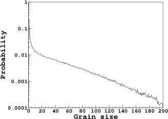
Figure 2: Plot of grain size distribution with mean grain size = 32.

To generate the grain configuration, we have take the following procedure. We start from an “unoccupied” AF lattice and insert $n_{\mbox{\tiny g}}$ seeds, where each seed is the starting point of a distinct grain. From these seeds, we grow grains by the following process. Randomly choose a site. If an empty site is chosen, choose another site. If the chosen site belongs to a grain, let all empty neighbors of this site belong to the same grain. Repeat this step until all sites are occupied. Fig. 2 shows the grain size distribution with 512 grains on $32\times 64\times 8$ lattice averaged over $512$ samples. Grain configurations with $512$ grains and average grain size of 32 lattice sites are used unless otherwise stated.

We derive a set of coupled mean-field equations for the magnetization of each AF grain. These equations account for the free surfaces and the surface fields due to interactions with other grains. Details of derivations will be shown elsewhere hkl . For the $j$th grain, it follows that

$$m^{\chi}_{j}\left[\frac{q}{2}(\rho_{Bj}^{\psi}+\rho_{Bj}^{\chi})+\frac{q_{\mbox{\tiny S}}}{2}(\rho_{Sj}^{\psi}+\rho_{Sj}^{\chi})\right]=$$ (3)

$$\rho_{Bj}^{\chi}q\tanh[\beta(J_{\mbox{\tiny AF}}qm^{\psi}_{j}+h)]+$$

$$\rho_{S\mbox{\tiny free}j}^{\chi}q_{\mbox{\tiny S}}\tanh[\beta(J_{\mbox{\tiny AF}}q_{\mbox{\tiny S}}m^{\psi}_{j}+h)]+$$

$$\rho_{S\mbox{\tiny FM}j}^{\chi}q_{\mbox{\tiny S}}\tanh[\beta(J_{\mbox{\tiny AF}}q_{\mbox{\tiny S}}m^{\psi}_{j}+h+J_{\mbox{\tiny I}}M^{x})]+$$

$$\sum_{k=1}^{n_{\mbox{\tiny g}}}\rho_{Sjk}^{\chi}q_{\mbox{\tiny S}}\tanh[\beta(J_{\mbox{\tiny AF}}q_{\mbox{\tiny S}}m^{\psi}_{j}+h+J_{\mbox{\tiny g}}q_{\mbox{\tiny g}}m^{\psi}_{k})]$$

where the variables $\psi$ and $\chi$ are used to represent sublattices, that is, $m^{\psi}_{j}$ and $m^{\chi}_{j}$ are the magnetization of one sublattice of the $j$th grain and that of the other sublattice, respectively. For each grain, there are a pair of symmetric equations for both sublattices. As a total, Eq. (3) consists of a set of $2n_{\mbox{\tiny g}}$ equations. The variables in Eq. (3) are defined as follows: $q=6$ is the coordination number in the bulk, $q_{\mbox{\tiny S}}$ is the average coordination number on the surface, $q_{\mbox{\tiny g}}$ is the average coordination number between sites belonging to different grains, and $\beta$ is the inverse temperature. By defining the densities of bulk/surface sites as the number of bulk/surface sites divided by the total number of sites in the simulation box, we express the mean-field equation in terms of densities. $\rho_{Bj}^{\psi/\chi}$ and $\rho_{Sj}^{\psi/\chi}$ are the densities of bulk sites and surface sites for sublattice $\psi/\chi$, respectively. $\rho_{S\mbox{\tiny free}j}^{\chi}$ is the density of free surface, $\rho_{S\mbox{\tiny FM}j}^{\chi}$ is the density of sites adjacent to the FM layer, and $\rho_{Sjk}^{\psi}$ is the density of surface sites adjacent to the neighboring $k$th grain. The first term in the right hand side of Eq.(3) gives the contribution to $m^{\chi}_{j}$ due to magnetization ordering in the bulk. The second term gives the contribution due to the free surfaces at $z=0$. The third term is due to interactions with the top FM layer and the last term is due to inter-grain interactions. For the FM layer the free energy is calculated as

$$f = \frac{J_{\mbox{\tiny FM}}q_{\mbox{\tiny FM}}M^{2}}{2}$$

$$-\frac{1}{\beta}\sum_{k}^{n_{\mbox{\tiny g}}}\left(\rho_{S\mbox{\tiny FM}k}^{\psi}\log(I[\vec{M},\vec{h}_{k}^{\psi}])+\rho_{S\mbox{\tiny FM}k}^{\chi}\log(I[\vec{M},\vec{h}_{k}^{\chi}])\right)$$

where $\vec{M}$ is the FM magnetization, $q_{\mbox{\tiny FM}}=4$ is the coordination number of FM layer, $\vec{h}_{k}^{\psi/\chi}$ is an effective field defined by $\vec{h}_{k}^{\psi/\chi}=(h+J_{\mbox{\tiny I}}m_{k}^{\psi/\chi})\hat{e}_{x}$. $I[\vec{M},\vec{h}_{k}^{\psi/\chi}]$ is an integral to be evaluated numerically,

$$I[\vec{M},\vec{h}]=\int_{4\pi}d\vec{s}\exp\left[\beta(J_{\mbox{\tiny FM}}q_{\mbox{\tiny FM}}\vec{M}+\vec{h})\cdot\vec{s}+\beta d(s^{x})^{2}\right]$$ (5)

The $x$ component of $\vec{M}$, $M^{x}$, appears in Eq. (3). Computation of mean-field magnetizations consists of solving Eq. (3) iteratively and simultaneously minimizing Eq. (Exchange Bias with Interacting Random Anti-ferromagnetic Grains).

Let us explain the field-cool process. From now on, we use dimensionless units with $J_{\mbox{\tiny FM}}=1$, and the temperature $T$ is given in units of $J_{\mbox{\tiny FM}}/k_{\mbox{\tiny B}}$, where $k_{\mbox{\tiny B}}$ is the Boltzmann constant. The system is first cooled under the field $h_{\mbox{\tiny cool}}$ from $T=5$ to $T=0.2$ in steps of $T_{i+1}=0.95T_{i}$. There are two possible domain orientations for the AF grains, with sublattice $\psi$ pointing in the $+1$ direction and $\chi$ pointing in the $-1$ direction, or vice versa. During the field-cool process, we attempt to obtain the global free energy minimum by considering two different domain orientations for each AF grain and pick up the one with lower free energy. At the end of the field-cool process, the temperature is kept constant and the field $h$ is reduced in steps of 0.01 and with a higher resolution near the region of magnetization reversal (0.002). At each step, the magnetization is calculated using the previous magnetization state as the starting values for Eq. (3) and Eq. (Exchange Bias with Interacting Random Anti-ferromagnetic Grains). In this way, meta-stable states can be traced out to obtain the hysteresis loop. We simulate the field-cool process and the hysteresis loop based on the mean-field equations.

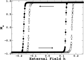
Figure 3: Hysteresis loop for $J_{\mbox{\tiny I}}=-0.5$ (white squares) and $J_{\mbox{\tiny I}}=0.5$ (black circles), with representative error bars obtained from 64 independent simulations.

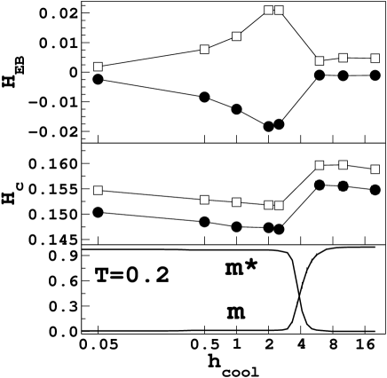
Figure 4: The dependence of $H_{\mbox{\tiny EB}}$ and $H_{\mbox{\tiny C}}$ on cooling field for $J_{\mbox{\tiny I}}=-0.5$ (white squares) and $J_{\mbox{\tiny I}}=0.5$ (black circles). The bottom plot shows the magnetization $m$ and staggered magnetization $m^{*}$ at the AF/FM interface at $T=0.2$.

Fig. 3 shows the hysteresis loops at $T=0.2$. Hysteresis loops shifted to the right for $J_{\mbox{\tiny I}}=-0.5$ (white squares) and left for $J_{\mbox{\tiny I}}=0.5$ (black circles). Field-cooling is performed at $h_{\mbox{\tiny cool}}=2$. The origin of the shift comes from excess magnetization in the AF bulk created during field-cooling. This result is consistent with the intuitive picture discussed by Nogués and Schuller nogues . The shift in hysteresis loop should depend on the magnetization state immediately before the hysteresis loop is traced out. We shall modify the magnetization state by using different cooling fields.

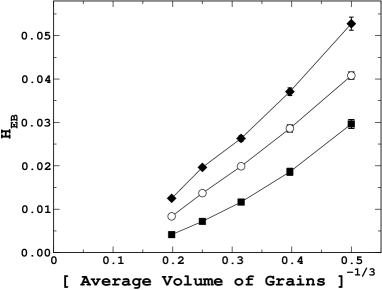
Figure 5: Grain size dependence of exchange bias for $J_{I}=-0.5,J_{g}=-0.15,h_{\mbox{\tiny cool}}=1.0$ (filled squares), $J_{I}=-0.5,J_{g}=-0.15,h_{\mbox{\tiny cool}}=2.0$ (empty circles), $J_{I}=-0.5,J_{g}=0,h_{\mbox{\tiny cool}}=1.0$ (filled diamonds). Error bars are smaller than the size of the symbols.

We performed a systematic study on the dependence of the exchange bias field $H_{\mbox{\tiny EB}}$ and coercivity $H_{\mbox{\tiny C}}$ in the field-cool process. $H_{\mbox{\tiny EB}}$ is defined as $(H_{+}+H_{-})/2$ where $H_{+}$ and $H_{-}$ are the fields at which the magnetization is zero in the hysteresis loop. Similarly, we define $H_{\mbox{\tiny C}}=(H_{+}-H_{-})/2$. Fig. 4 shows that $H_{\mbox{\tiny EB}}$ increases from zero to a maximum at about $h_{\mbox{\tiny cool}}=2.5$ and decreases at $h_{\mbox{\tiny cool}}>6$. The hysteresis loop remains unshifted with $h_{\mbox{\tiny cool}}=0$ when cooled from a demagnetized state; this observation is consistent with experiments on exchange bias meiklejohn ; takahashi ; steams . Increase and decrease of $H_{\mbox{\tiny EB}}$ and $H_{\mbox{\tiny C}}$ with cooling field is also reported in real materials such as Ni/NiFe₂O₄ negulescu and permalloy/CoO timothy ; ambrose . As shown in the bottom plot of Fig. 4, at $h<2.5$, the spins of AF-FM interface are locked in a magnetization state with staggered magnetization $m^{*}\approx 1$, and at $h>6$, the staggered magnetization vanishes. Our result shows that cooling field of $h_{\mbox{\tiny cool}}=2.5$, for the sets of parameters used in the present study, produces maximum excess magnetization in the AF-FM interface while maintaining non-zero staggered magnetization, causing a maximum exchange bias. At higher cooling field, spins in the AF material are aligned during field-cooling; when the field is decreased to sweep the hysteresis loop, the AF grains get locked in AF states with random domain orientations that generate little excess magnetization. Hence there is a close relationship between the magnetization state of the AF/FM interface and $H_{\mbox{\tiny EB}}$. We also found, as in timothy , that there is a decrease of coercivity corresponding to an increase of exchange bias. The dependence of exchange bias on cooling field is of particular importance in fabrication of exchange bias devices where tuning of exchange bias is desirable.

Fig. 5 shows grain size dependence of exchange bias. Average grain sizes of 8, 16, 32, 64 and 128 are used. Simulations with interacting/non-interacting grains and different cooling fields were performed. The exchange bias field is inversely proportional to the grain diameter $D$, $H_{\mbox{\tiny EB}}\sim 1/D$. For non-interacting grains (filled diamonds) and strong cooling field (empty circles), plots of exchange bias versus inverse grain diameter $D^{-1}$ fall on a straight line very well. For smaller cooling fields (filled squares), exchange bias goes to zero asymptotically at large grain sizes. Simulations with $J_{I}=-0.75$ were also performed and the exchange bias field changes only slightly compared to simulations with $J_{I}=-0.5$. This inverse relationship of exchange bias on grains size is also reported in exchange bias systems of permalloy/CoO bilayers takano and Cr₇₀Al₃₀/Fe₁₉Ni₈₁ bilayers uyama .

Other models has been developed to describe the mechanism of unidirectional anisotropy. Stiles and McMichael stiles used an ordered granular model to explain exchange bias through partial domain wall formation. Scholten et al. scholten used mean-field equations on local magnetization to explain the domain state model. The model presented here is distinct from all previous models. The mean-field equations for an explicit grain distribution has been given for the first time in this paper, and the domain state model is realized explicitly by actual grain distribution.

To summarize, we developed a simple model that captures many features of real exchange bias systems. We found a direct relationship between the cooling field dependence of the exchange bias, coercivity and magnetization states on the AF-FM interface. We also verified that the exchange bias field is inversely proportional to the AF grain sizes and this relationship is independent of the inter-grain interactions, AF/FM interactions and cooling fields. Lastly, we would like to mention that the simulations based on mean-field equations used in this paper are general, and may be used to study other exchange bias parameters, such as surface roughness, perpendicular coupling and film thickness.

This work is supported by a Grant-in-Aid for Scientific Research from the Japan Society for the Promotion of Science. The computation of this work has been done using computer facilities of the Supercomputer Center, Institute of Solid State Physics, University of Tokyo.

References

- (1) H. Meiklejohn and C. P. Bean, Phys. Rev. 102, 1413 (1956).
- (2) J. Nogués and I. K. Shuller, J. Magn. Magn. Mater. 192, 203 (1999).
- (3) U. Nowak, A. Misra and K. D. Usadel, J. Magn. Magn. Mater. 240, 243 (2002).
- (4) J. R. L. de Almeida and S. M. Rezende, Phys. Rev. B 65, 092412 (2001).
- (5) P. Miltényi, M. Gierlings, J. Keller, B. Beschoten, G. Güntherodt, U. Nowak and K. D. Usadel, Phys. Rev. Lett. 84, 4224 (2000); B. Beckmann, U. Nowak and K. D. Usadel, Phys. Rev. Lett. 91, 187201 (2003).
- (6) G. Scholten, K. D. Usadel, U. Nowak, Phys. Rev. B 71, 064413 (2005).
- (7) H. K. Lee and Y. Okabe, In preparation.
- (8) M. Takahashi, A. Yanai, S. Taguchi and T. Suzuki, Jpn. J. Appl. Phys. 19, 1093 (1980).
- (9) M. B. Steams, J. Appl. Phys. 55, 1729 (1984).
- (10) C. Negulescu, L. Thomas, M. Guyot and C. Papusoi, J. Optoelectronics Adv. Mater. 6, 719 (2004).
- (11) T. J. Moran and I. K. Schuller, J. Appl. Phys. 79, 5109 (1996).
- (12) T. Ambrose and C. L. Chien, J. Appl. Phys. 83, 7222 (1998).
- (13) K. Takano, R. H. Kodama, A. E. Berkowitz, W. Cao and G. Thomas, Phys. Rev. Lett. 79, 1130 (1997).
- (14) H. Uyama, Y. Otani, K. Fukamichi, O. Kitakami, Y. Shinmada and J-i Echigoya, Appl. Phys. Lett. 71, 1258 (1997).
- (15) M. D. Stiles and R. D. McMichael, Phys. Rev. B 59, 3722 (1999).