Stoke’s efficiency of temporally rocked ratchets

Abstract

We study the generalized efficiency of an adiabatically rocked ratchet with both spatial and temporal asymmetry. We obtain an analytical expression for the generalized efficiency in the deterministic case. Generalized efficiency of the order of $50\%$ is obtained by fine tuning of the parameter range. This is unlike the case of thermodynamic efficiency where we could readily get an enhanced efficiency of upto $90\%$. The observed higher values of generalized efficiency is attributed to be due to the suppression of backward current. We have also discussed briefly the differences between thermodynamic, rectification or generalized efficiency and Stoke’s efficiency. Temperature is found to optimize the generalized efficiency over a wide range of parameter space unlike in the case of thermodynamic efficiency.

I Introduction

Nonequilibrium fluctuations can induce directed transport along periodic extended structures without the application of a net external bias. Diverse studies exist in literature which centralize on this phenomena of noise induced transport julicher ; reiman ; 1amj ; special . The extraction of useful work by the rectification of thermal fluctuations inherent in the medium at the expense of an overall increase in the entropy of the system plus the environment parrondo ; demon ; 2amj have become a major area of research in nonequilibrium statistical mechanics. The key criterion for the possibility of such a transport are the presence of unbiased nonequilibrium perturbations and a broken spatial or temporal symmetry. With the increase in prominence of the study of nano-size particles, the concurrent thermal agitations can no longer be ignored. The perceptivity of the basic mechanism of ratchet operation has been disclosed through various models like flashing ratchets, rocking ratchets, time asymmetric ratchets, frictional ratchets etc julicher ; reiman ; 1amj ; special .

Extensive studies have been done to understand the nature of currents, their possible reversals and also the efficiency of energy transduction. These results are of immense utilization in the development of proper models that efficiently separate particles of micro and nano sizes and also in turn for the development of machines at nano scales raishma-natl . Processes in which the chemical energy stored in a nonequilibrium bath is transformed into useful work are believed to be the basis of molecular motors and are of great importance in active biological processes.

With the development of a separate subfield called stochastic energetics sekimoto ; parrondo , the reaction force exerted by the stochastic system on the bath is identified with the heat discarded by the system to the bath. With this definition, it has become possible to establish the compatibility between the Langevin or Fokker-Planck formalism with the laws of thermodynamics. This framework helps to calculate various physical quantities like efficiency of energy transduction kamgawa , energy dissipation (hysteresis loss), entropy production rkamj etc., thereby rendering a new tool to study systems far from equilibrium.

In the present work we consider time asymmetric ratchet  pre ; chialvo ; ai where the ratchet potential is rocked adiabatically in time in such a way that a large force field $F(t)$ acts for a short time interval of period in the forward direction as compared to a smaller force field for a longer time interval in the opposite direction. The intervals are so chosen that the net external force or bias acting on the particle over a period is zero. With such a time asymmetric forcing, one can generate enhanced unidirectional currents even in the presence of a spatially symmetric periodic potential chialvo .

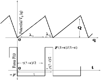
Figure 1: Plot of sawtooth potential as a function of coordinate $q$ and the time asymmetric forcing $F(t)$ as a function of $t$.

The schematic figure of the ratchet potential $V_{0}(q)$ chosen for our present work and the time asymmetric forcing $F(t)$ are shown in Fig. 1. Time asymmetric forcing can also be generated by applying a biharmonic force or harmonic mixing  marchi . Theoretically, time asymmetric ratchets have been considered in earlier literatures under different physical contexts  save ; chacon . Several experimental studies have also been explored such as generation of photo-currents in semiconductors  shmelev , transport in binary mixtures save , realization of Brownian motors using cold atoms in a dissipative optical lattice schiavoni etc.

One of the key concepts in the study of the performance characteristics of Brownian engines/ratchets is the notion of efficiency of energy transduction from the fluctuations linke . The primary need for efficient motors arises either to decrease the energy consumption rate and/or to decrease the heat dissipation in the process of operations and it is the latter concept which is of more importance in the present world of miniaturization of components parrondo . As the ratchet operates in a nonequilibrium state there is always an unavoidable and irreversible transfer of heat via fluctuations (in coordinate and accompanying velocity) thereby making it less efficient as a motor. Any irreversibility or finite entropy production will reduce the efficiency. For instance, the attained value of thermodynamic efficiency in flashing and rocking ratchet are below the subpercentage regime ($<0.01$). However, it has been shown that at very low temperatures fine tuning of parameters could easily lead to a larger efficiency, the regime of parameters being very narrow sokolov . Protocols to optimize the efficiency in saw tooth ratchet potential in presence of spatial symmetry and symmetric temporal rocking have been worked out in detail in sokolov ; hernandez .

By construction of a special type of flashing ratchet with two asymmetric double-well periodic-potential states displaced by half a period tsong a high efficiency of an order of magnitude higher than in earlier models  sekimoto ; parrondo ; kamgawa ; astu05 were obtained. The basic essence here was that even for diffusive Brownian motion the choice of appropriate potential profile ensures suppression of backward motion leading to a reduction in the accompanying dissipation. Similar to the case of flashing ratchets  tsong we had earlier studied the motion of a particle in a rocking ratchet by applying a temporally asymmetric but unbiased periodic forcing in the presence of a sinusoidal pre and saw tooth potential jstat . The efficiency obtained was very high, much above the subpercentage level, about $\sim 30-40\%$, without fine tuning for the case of sinusoidal and $\sim 90\%$ for the saw tooth case in the presence of temporal asymmetry.

It is to be pointed that in all ratchet models the particles move in a periodic potential system and hence it ends up with the same potential energy even after crossing over to the adjacent potential minimum. There is no extra energy stored in the particle which can be usefully expended when needed. Hence to have an engine out of a ratchet it is necessary to use its systematic motion to store potential energy which inturn is achieved if a ratchet lifts a load  parrondo ; kamgawa-parrondo . Thus a load force $L$ is applied in a direction opposite to the direction of current in the ratchet. With this definition, the thermodynamic efficiency assumes a zero value when no load force is acting parrondo ; machura .

However, as not all motors are designed to pull the loads alternate proposals for efficiency have come up depending on the task the motor have been proposed to do without taking recourse to the application of a load force. Some motors may have to achieve high velocity against a frictional drag. This consecutively implies that the objective of the motor considered is to move a certain distance in a given time interval with minimal fluctuations in velocity and its position. In such a case one defines the generalized efficiency derenyi or rectification efficiency munakata which in the absence of load is sometimes called as Stokes efficiency oster , given by the expression

$$\eta_{S}=\frac{E_{min}}{E_{in}}.$$ (1)

$E_{min}=\gamma<v>^{2}$ is the minimum average power necessary to maintain the motion of the motor with an average velocity $<v>$ against an opposing frictional force. $E_{in}$ is the average input power. In the presence of load the generalized efficiency or rectification efficiency is defined as  machura1 ; derenyi ; munakata , $\eta_{g-r}$

$$\eta_{g-r}=\frac{L<v>+\gamma<v>^{2}}{E_{in}}$$ (2)

The numerator in the above equation is the sum of the average power necessary to move against the external load and against the frictional drag with velocity $<v>$ respectively. The thermodynamic efficiency of energy transduction is given by

$$\eta_{t}=\frac{L<v>}{E_{in}}.$$ (3)

This definition can be used for the overdamped munakata as well as in the underdamped case machura . For the case of underdamped Brownian motor there is an added advantage that the input power can be written in terms of experimentally observable quantities namely, $<v>$ and its fluctuations machura ; munakata . This is independent of the model of the ratchet chosen.

In the present work we mainly analyze the nature of generalized efficiency in the absence of load, namely Stoke’s efficiency. The behavior in presence of load is also briefly discussed. We obtain values of Stoke’s efficiency of the order of $50\%$ by fine tuning the parameters. In the generic parameter space, we obtain efficiencies much above the sub percentage regime. The earlier model for the case of flashing ratchet munakata gave a generalized efficiency of the order of $0.2$. In a recent study machura2 , it has been shown that Stoke’s efficiency exhibits a high value of around $0.75$, when the motor operates in an inertial regime and at very low temperatures. However, these inertial motors do not exhibit high thermodynamic efficiency. We also show that unlike thermodynamic efficiency, the generalized efficiency is aided or optimized by temperature.

Our paper is organized as follows. We first describe our model in Section II. Results and discussions are given in Section III which is consecutively followed by conclusions in Section IV.

II The Model:

Our model consists of an overdamped Brownian particle with co-ordinate $q(t)$ in a spatially asymmetric potential $V(q)$ subjected to a temporally asymmetric rocking. The stochastic differential equation or the Langevin equation for such a particle is given by overdamp

$${\dot{q}}={-{\frac{(V^{\prime}(q)-F(t))}{\gamma}}}+\xi(t),$$ (4)

with $\xi(t)$ being the randomly fluctuating Gaussian thermal noise having zero mean and correlation, $<\xi(t)\xi(t^{\prime})>\,=\,(2\,{k_{B}T}/\gamma)\delta(t-t^{\prime})$ with $\gamma$ being the friction coefficient. We consider in the present work a piecewise linear ratchet potential as in the case of Magnasco  magnasco with periodicity $\lambda=\lambda_{1}+\lambda_{2}$ set equal to unity, Fig. 1 . This also corresponds to the spacing between the wells. We later on scale all the lengths with respect to $\lambda$.

$$V(q) = \frac{Q}{\lambda_{1}}q,\,\,\,\,\,\,\,\,q\leq\lambda_{1}$$ (5)

$$= \frac{Q}{\lambda_{2}}(1-q),\,\,\lambda_{1}<q\leq\lambda$$

$F(t)$ which is the externally applied time asymmetric force with zero average over the period is also shown in Fig. 1. The force in the gentler and steeper side of the potential are respectively $f^{+}=\frac{-Q}{\lambda_{1}}$ and $f^{-}=\frac{Q}{\lambda_{2}}$ and $Q$ is the height of the potential.

We are interested in the adiabatic rocking regime where the forcing $F(t)$ is assumed to change very slowly, i.e., its frequency is smaller than any other frequency related to the relaxation rate in the problem such that the system is in a steady state at each instant of time.

Following Stratonovich interpretation stratanovich , the corresponding Fokker-Planck equation riskin is given by

$$\frac{\partial P(q,t)}{\partial t} = \frac{\partial}{\partial q}\Big{[}k_{B}T\frac{\partial P(q,t)}{\partial q}$$

$$+ [V^{\prime}(q)-F(t)+L]P(q,t)\Big{]}.$$

The probability current density $j$ for the case of constant force (or static tilt) F is given by

$$j(F_{0})=\frac{{P_{2}}^{2}\sinh\{\lambda[F_{0}-L]/2k_{B}T\}}{{{k_{B}T{(\lambda/Q)}^{2}}P_{3}}-{(\lambda/Q)P_{1}P_{2}\sinh\{\lambda[F_{0}-L]/2k_{B}T\}}}$$ (7)

where

$$P_{1} = \Delta+\frac{\lambda^{2}-\Delta^{2}}{4}\frac{F_{0}-L}{Q}$$ (8)

$$P_{2} = (1-\frac{\Delta[F_{0}-L]}{2Q})^{2}-(\frac{\lambda[F_{0}-L]}{2Q})^{2}$$ (9)

$$P_{3} = \cosh(\{Q-\Delta/2[F_{0}-L]\}/k_{B}T)-$$ (10)

$$\mbox{}\cosh\{\lambda[F_{0}-L]/2k_{B}T\}$$

where $\Delta=\lambda_{1}-\lambda_{2}$ is the spatial asymmetry factor. In the above expression we have also included the presence of an external load $L$, which is essential for defining thermodynamic efficiency. The current in the stationary adiabatic regime averaged over the period $\tau$ of the driving force $F(t)$ is given by

$$<j>=\frac{1}{\tau}\,\int_{0}^{\tau}\,j(F(t))\,dt.$$ (11)

The form of the time asymmetric ratchets with a zero mean periodic driving force that we have chosen  pre ; chialvo ; ai is given by

$$F(t) = \frac{1+\epsilon}{1-\epsilon}\,F,\,\,(n\tau\leq t<n\tau+\frac{1}{2}\tau(1-\epsilon)),$$

$$= -F,\,\,(n\tau+\frac{1}{2}\tau(1-\epsilon)<t\leq(n+1)\tau).$$

Here, the parameter $\epsilon$ signifies the temporal asymmetry in the periodic forcing, $\tau$ the period of the driving force $F(t)$ and $n=0,1,2....$ is an integer. For this forcing in the adiabatic limit the expression for time averaged current is chialvo ; kamgawa

$$<j>=j^{+}+j^{-}\,,$$ (13)

with

$$j^{+} = \frac{1}{2}(1-\epsilon)\,j(\frac{1+\epsilon}{1-\epsilon}F)\,,$$ (14)

$$j^{-} = \frac{1}{2}(1+\epsilon)\,j(-F)$$

where $j^{+}$ is the current fraction in the positive direction over a fraction of time period $(1-\epsilon)/2$ of $\tau$ when the external driving force field is $(\frac{1+\epsilon}{1-\epsilon})F$ and $j^{-}$ is the current fraction over the time period $(1+\epsilon)/2$ of $\tau$ when the external driving force field is $-F$. The input energy $E_{in}$ per unit time is given by kamgawa ; pre

$$E_{in}=F[(\frac{1+\epsilon}{1-\epsilon})j^{+}-j^{-}].$$ (15)

In order for the system to do useful work, a load force $L$ is applied in a direction opposite to the direction of current in the ratchet. The overall potential is then $V(x)=-[V_{0}(x)-xL]$. As long as the load is less than the stopping force $L_{s}$ current flows against the load and the ratchet does work. Beyond the stopping force the current flows in the same direction as the load and hence no useful work is done. Thus in the operating range of the load, $0<\,L<\,L_{s}$, the Brownian particles move in the direction opposite to the load and the ratchet does useful work kamgawa-parrondo . The average rate of work done over a period is given by kamgawa

$$E_{out}=L[j^{+}+j^{-}]\,.$$ (16)

The thermodynamic efficiency of energy transduction is  sekimoto ; parrondo

$$\eta_{t}=\frac{L[j^{+}+j^{-}]}{F[(\frac{1+\epsilon}{1-\epsilon})j^{+}-j^{-}]}.$$ (17)

At very low temperatures or in the deterministic limit and also in the absence of applied load, the barriers in the forward direction disappears when $\frac{(1+\epsilon)}{(1-\epsilon)}F>\frac{Q}{\lambda_{1}}$ or $F>\frac{Q(1-\epsilon)}{\lambda_{1}(1+\epsilon)}$, and a finite current starts to flow in the forward direction. When $F>Q/\lambda_{2}$, the barriers in the backward direction also disappears and hence we now have a current in the backward direction as well leading to a decrease in the average current. In between the above two values of $F$, the current increases monotonically and peaks around $Q/\lambda_{2}$. In this range, a high efficiency is expected sokolov ; rkamj ; pre ; jstat . In the limit when there is only forward current in the ratchet i.e. $j^{+}>>j^{-}$ and $L=0$ generalized efficiency reduces to Stoke’s efficiency and is given by

$$\eta_{S}=\frac{(1-\epsilon)j^{+}}{(1+\epsilon)F}.$$ (18)

In the present work we mainly focus on the case when the load $L=0$.

For the case of adiabatic rocking the ratchet can be considered as a rectifier sokolov and in the deterministic limit of operation and with zero applied load when $F$ is in the range $\frac{Q}{\lambda_{2}}>F>\frac{Q(1-\epsilon)}{\lambda_{1}(1+\epsilon)}$, finite forward current alone exists and the analytic expression for current is given by

$$j^{+}=\frac{1}{2}{\Big{[}{\frac{\lambda_{1}^{2}}{(1+\epsilon)F\lambda_{1}-Q(1-\epsilon)}+\frac{\lambda_{2}^{2}}{(1+\epsilon)F\lambda_{2}+Q(1-\epsilon)}}\Big{]}}^{-1}$$ (19)

Thus, Eqns. 18 and  19 give an analytical expression for the Stoke’s efficiency in the deterministic limit. We take all physical quantities in dimensionless units. The energies are scaled with respect to the height of the ratchet potential, $Q$; all lengths are scaled with respect to the period of the potential, $\lambda$, which is taken to be unity and we also set $\gamma=1$ . In the following section we present our results followed by discussions pre ; jstat ; overdamp .

III Results and Discussions

Figure 2: Plot of efficiency as a function of $F$ at $T=0.01$ for different $\epsilon$ values with $\Delta=0.0$. Inset shows the behavior of current for the parameters given in the figure

Figure 3: Plot of efficiency as a function of $F$ at $T=0.01$ for different $\epsilon$ values $\Delta=0.9$. Inset shows the behavior of current for the parameters given in the figure.

In Fig. 2 and Fig.3 we plot generalized efficiency in the absence of load or Stoke’s efficiency as a function of $F$ for different values of $\epsilon$ at $T=0.01$ for symmetric $\Delta=0.0$ and asymmetric potential $\Delta=0.9$ respectively. As we increase $F$ in the interval from zero to $F_{min}=\frac{Q(1-\epsilon)}{\lambda_{1}(1+\epsilon)}$ the current is almost zero since barriers to motion exist in both forward (right) and backward (left) directions. This critical value of $F$ will decrease as we increase $\epsilon$ as seen from Figs. 2 and  3. For $F>F_{min}$ barriers to the right disappears and as a consequence the current (inset) increases as a function of $F$ till $F_{max}=\frac{Q}{\lambda_{2}}$ beyond which the current also starts flowing in the backward direction. The behaviour of Stoke’s efficiency reflects the nature of current (cf Eqn. 18). Note that the value of $F_{max}$ does not depend on the time asymmetry parameter $\epsilon$, as is clear from Figs. 2 and  3. Beyond $F_{max}$, barriers to motion in both the directions disappear and currents as well as generalized efficiency starts decreasing beyond $F_{max}$. We have seen that input energy increases monotonically with $F$ for all the parameters. Hence the qualitative behaviour of current is reflected in the nature of generalized efficiency. From the plot we see that the dependence of generalized efficiency on $\epsilon$ is not in a chronological manner. High $\epsilon$ value need not correspond to high generalized efficiency. For a given $\epsilon$ the current and Stoke’s efficiency exhibits a peak around $F_{max}$.

We see from Eqn. 19 that for $\lambda_{1}>>\lambda_{2}$ (i.e., large spatial asymmetry) and $F_{min}<F<F_{max}$, the analytical results from Eqn. 19 for the forward current fraction is simply given by $j_{+}=\frac{(1+\epsilon)F}{2\lambda_{1}}$, while the Stoke’s efficiency becomes $\eta_{S}=\frac{1-\epsilon}{2\lambda_{1}}$. It is obvious from Fig. 3 that in this domain, $j+$ is a linear function of $F$ (inset) while $\eta_{S}$ exhibits a plateau in this regime. This plateau regime is clearly observable for $\epsilon=0.9$ and $\Delta=0.9$ as in Fig.3. For these parameters, the ranges between $F_{min}$ and $F_{max}$ is large and moreover $\lambda_{1}>>\lambda_{2}$. The value of $\eta_{S}$ at the plateau is $0.05$, which is consistent with the analytical result.

Figure 4: Plot of Stoke’s efficiency as a function of $\epsilon$ at $T=0.01$ for $F=0.5$ and $1.5$ for $\Delta=0.0$. Inset shows the behaviour of efficiency for $F=0.5\,,\,1.5$ and $F=5.0$ but with $\Delta=0.9$ for the parameters given in the figure.

In contrast to the nature of $\eta_{S}$, we see that the average current, for a given $F$ and $\Delta$, always increases as $\epsilon$ is increased, see insets of Figs. 2 and 3. However, we see from Eqn. 18 that $\eta_{S}$ also depends on $\epsilon$ through the factor $\frac{(1-\epsilon)}{(1+\epsilon)}$ which is a decreasing function of $\epsilon$ and hence the existence of optimal value of $\epsilon$ for $\eta_{S}$ is understandable. For a large spatial asymmetry, $\Delta=0.9$, in the ratchet potential the magnitude of the average currents are quite large even for given $\epsilon$ as compared to the case when $\Delta$ is small.

From Fig. 2 we notice that the optimum value of generalized efficiency obtained is around $20\%$. This is the case of symmetric potential driven by temporally asymmetric force. From Fig. 3, we notice that the inclusion of spatial asymmetry in the potential helps in enhancing the generalized efficiency and we can obtain an optimal value of nearly $50\%$ for efficiency in a particular parameter space.

In Fig. 4 we plot the generalized efficiency with zero load (or Stoke’s efficiency $\eta_{S}$) as a function of $\epsilon$ for different $F$ and symmetric potential. We have taken $T=0.01$ so as to be closer to the deterministic limit. The inset shows the same plot with asymmetric potential. We observe that for a given value of $F$, only those $\epsilon$ values contribute to $\eta_{S}$ for which $F>F_{min}$. The minimum value of $\epsilon$ is given by $\epsilon_{min}=\frac{(Q-\lambda_{1}F)}{(Q+\lambda_{1}F)}$. For larger $F$, $\epsilon_{min}$ shifts to a smaller value as can be seen easily from the figure. Moreover from Eqn.18 we can see that as $\epsilon$ approaches 1, the $\eta_{S}$ approaches zero (even though, strictly speaking, the $\epsilon\rightarrow 1$ limit is pathological). Thus, for the chosen parameter values the $\eta_{S}$ exhibits a peaking behavior. Note that the current vanishes due to the spatial symmetry of the potential in the limit $\epsilon\rightarrow 0$.

We now study the case when there is a spatial asymmetry which is shown in the inset of Fig. 4. Here, a finite current can arise even when $\epsilon=0$ provided force $F>\frac{Q}{\lambda_{1}}$. Thus $\eta_{S}$ in this regime can have finite value at $\epsilon=0$ and can show a peaking behaviour. For $F>>\frac{Q}{\lambda_{1}}$, efficiency shows a monotonically decreasing behavior as a function of $\epsilon$. This clearly brings out the fact that in certain parameter ranges, time-asymmetric driving need not help in enhancing $\eta_{S}$ in the presence of spatially asymmetric potential. In the range $F<\frac{Q}{\lambda_{1}}$, currents are zero at $\epsilon=0$; thus $\eta_{S}$ exhibits a peaking behaviour with a value of zero for $\epsilon=0$ and $\epsilon=1$ in accordance with Eqn. 18. These results show that $\eta_{S}$ is not a monotonically increasing function of $\epsilon$.

Figure 5: Efficiency as a function of temperature for $F=1.0$ and $\epsilon=0.2$ for varying $\Delta$. Inset shows the behaviour of current with temperature for the same set of parameters.

We next discuss the behaviour of $\eta_{S}$ with temperature. In Fig. 5 we plot $\eta_{S}$ as a function of temperature for a fixed $F=0.1$ and temporal asymmetry $\epsilon=0.9$ but with varying potential asymmetry $\Delta$. In most of the generic parameter space, we observe that temperature (or noise) facilitates $\eta_{S}$ which quite is opposite to the generically observed behavior of thermodynamic efficiency jstat . For example, if we take a particular curve say, $\Delta=0.0,F=0.1,\epsilon=0.9$, we can see that the value of efficiency is zero at $T=0$. This is because of the presence of the barriers in either directions during rocking. Thus when $F<F_{min}$, efficiency (current) is zero and as temperature is increased current starts to build up since Brownian particles can readily overcome the barriers to the right in the adiabatic limit. Beyond a certain $T$, current or efficiency will start to subside again as too much of noise will help the particle to overcome the barriers in both directions, thereby reducing the ratchet effect. Hence both current and generalized efficiency will fall. Thus for $F<F_{min}$ temperature always facilitates $\eta_{S}$.

Figure 6: Plot of thermodynamic efficiency, input energy, current and output energy as a function of load for $\epsilon=0.9$, $F=0.1$, $\Delta=0.9$ and $T=0.01$. The $E_{out}$ is scaled by a factor of $10$ to make it comparable to the scale chosen. Inset shows a comparison of the behaviour of thermodynamic, generalized and Stoke’s efficiency for the same set of parameter values.

With increase in spatial asymmetry we see a finite current even when temperature is zero. This is because of the disappearance of the barriers to motion in the forward direction. However Stokes efficiency increases and shows a peaking behavior as a function of temperature even in this range. In Fig. 5 note that peak value of current (inset) shifts to the right as we increase $\Delta$. With increase in $\Delta$ barriers to the left increases and hence to overcome these larger barriers higher temperature is required. Only above these temperatures does current in backward direction begin to flow causing decrease of average current. Hence it is understandable that peak in average current shifts to higher $T$ with increase in $\Delta$.

When $F>F_{max}$, the barriers in both directions disappear. We have separately verified that in this case both $\eta_{S}$ and the net current decreases monotonically as a function of temperature.

In the end we discuss briefly the differences between the nature of thermodynamic efficiency ($\eta_{t}$), generalized efficiency ($\eta_{g-r}$) and stokes efficiency ($\eta_{S}$). For the sake of comparison, we apply a load to the system. In Fig. 6 we plot the $\eta_{t}$, net current $<j>$, input ($E_{in}$) and output ($E_{out}$) power as a function of load for $\epsilon=0.9$, $\Delta=0.9$, $F=0.1$ and $T=0.01$. In the inset we plot the $\eta_{g-r}$, $\eta_{S}$ and $\eta_{t}$ as a function of load for the same set of parameters so as to have a comparative idea of the behaviour of the different definitions of efficiency.

We notice that the thermodynamic efficiency increases with load from zero and exhibits a high value ($90\%$) just before the stopping force or critical load, the range within which $\eta_{t}$ is defined. In contrast, $\eta_{S}$ (shown in the inset) has a finite value even when the load force is zero and then decreases monotonically with load. $\eta_{S}$ is almost zero and so is the velocity and current in the range where $\eta_{t}$ is very high. The magnitudes of current, $\eta_{S}$, $E_{in}$ and $E_{out}$ are very small near the stopping force, and hence are not observable on Fig. 6 due to the scale used. Both $\eta_{g-r}$ or $\eta_{S}$ starts with a finite value when load $L=0$ and it differs from $\eta_{t}$ in the low load limit. When the load value increases, $\eta_{g-r}$ also increases and at larger values of $L$ (near stopping force) it coincides with $\eta_{t}$. The main contribution to $\eta_{g-r}$ comes essentially from the work done against the load since velocity of particle is almost negligible and thus average power needed to move against the frictional drag becomes very small.

Another observation is that the average work done exhibits a peaking behavior where the thermodynamic efficiency is small and it is vanishingly small where the latter peaks. The average input power and current monotonically decreases with the load. The figure clearly indicates that high thermodynamic efficiency does not lead to higher currents / work / Stoke’s efficiency. These results clearly bring out glaring differences between different definitions of efficiency as they are based on physically different criteria of motor performance  derenyi ; munakata ; munakata1 ; machura2 .

IV Conclusions

We have studied the generalized efficiency in an adiabatically rocked system in the presence of spatial and temporal asymmetry. The Stoke’s efficiency exhibits a value of $50\%$ by fine tuning the parameters. Moreover, in a wide range of parameters this efficiency is much above the subpercentage regime. We have shown that in a wider parameter space temporal asymmetry may or may not facilitate the generalized efficiency whereas generically, temperature facilitates it. In the regime of parameter space where the current is zero in the deterministic limit, temperature always facilitates Stoke’s efficiency. In contrast, if the current is non-zero in the deterministic regime, depending on the parameters, it may happen that Stoke’s efficiency monotonically decreases with temperature. The obtained high values for both the thermodynamic and generalized efficiency is attributed to the effect of suppression of current in the backward direction. Recently, it has also been shown that the same effect in these ratchet systems leads to enhanced coherency or reliability in transport. unpub . In conclusion, in suitable parameter ranges, our system exhibits high values for all the performance characteristics, namely, Stoke’s efficiency, thermodynamic efficiency along with a pronounced transport coherency.

V Acknowledgement

One of us (AMJ) thanks Dr. M. C. Mahato for useful discussions.

References

- (1) F. Jülicher, A. Ajdari and J. Prost, Rev. Mod. Phys. 69, 1269 (1997).
- (2) P. Reimann, Phys. Rep. 361, 57 (2002) and references therein.
- (3) A. M. Jayannavar, Frontiers in Condensed Matter Physics, Vol 5, p215, ed. J. K. Bhattacharjee and B. K. Chakrabarti, Allied Publishers, India (2005); cond-mat 0107079.
- (4) Special issue on “Ratchets and Brownian motors: basics, experiments and applications” ed. H. Linke, Appl. Phys. A75(2) 2002.
- (5) J. M. R. Parrondo and B. J. De Cisneros, Appl. Phys. A75, 179 (2002).
- (6) M. M. Millonas, Phys. Rev. Lett. 74 p10 (1995); 75 p3027 (1997).
- (7) A. M. Jayannavar, Phys Rev E53, p2957 (1996).
- (8) Raishma Krishnan and A. M. Jayannavar, Natl. Acad. Sci. Lett. 27, 301 (2004).
- (9) K. Sekimoto, J. Phys. Soc. Jpn. 66, 6335 (1997).
- (10) F. Takagi and T. Hondou, Phys. Rev. E60, 4954 (1999); D. Dan, M. C Mahato and A. M. Jayannavar, Int. J. Mod. Phys B,14, 1585, (2000); D. Dan, Mangal C Mahato and A. M. Jayannavar, Physica A, 296, 375 (2001); K. Sumithra and T. Sintes, Physica A, 297, 1 (2001); D. Dan and A. M. Jayannavar, Phys. Rev. E66, 41106 (2002).
- (11) Raishma Krishnan and A. M. Jayannavar, Physica A, 345, 61 (2005).
- (12) Raishma Krishnan, Mangal C. Mahato and A. M. Jayannavar, Phys. Rev. E70, 21102 (2004).
- (13) D. R. Chialvo, M. M. Millonas, Phys. Lett. A 209, 26 (1995); M. C. Mahato and A. M. Jayannavar, Phys. Lett. 209 21 (1995); A. Adjari, D. Mukamel, L. Peliti and J. Prost, J. Phys., 1 (France) 4 1551 (1994).
- (14) Bao-Quan Ai, X. J. Wang, G. T. Liu, D. H. Wen, H. Z. Xie, W. Chen and L. G. Liu, Phys. Rev. E68, 061105 (2003).
- (15) F. Marchesoni, Phys. Lett. A, 119 221 (1986).
- (16) S. Savel’ev, F. Marchesoni, P. Hänggi and F. Nori, Europhys Lett 67 179(2004); Phys. Rev. E 70 066109 (2004); Euro. Phys. J. B 40 403 (2004).
- (17) R. Chacon and R. Quintero, Preprint physics/0503125 and references therein.
- (18) G. M. Shmelev, N. H. Song and G. I. Tsurkan, Sov. Phys. J. (USA), 28 161(1985); M. V. Entin, Sov. Phys. Semicond. 23 664(1989); R. Atanasov, A. Haché, J. L. P. Hughes, H. M. vanDriel and J. E. Sipe, Phys. Rev. Lett. 76 1703(1996); A. Haché, Y. Kostoulas,R. Atanasov, J. L. P. Hughes, J. E. Sipe and H. M. van Driel, Phys. Rev. Lett. 78 306(1997); K. N. Alekseev, M. V. Erementchouk and F. V. Kusmartsev, Europhys. Lett. 47 595(1999)
- (19) M. Schiavoni, L. Sanchez-Palencia, F. Renzoni and G. Grynberg, Phys. Rev. Lett.90 094101(2003) and references therein; P. H. Jones, M. Goonasekera and F. Renzoni, Phys. Rev. Lett. 93 073904(2004); R. Gommers, P. Douglas, S. Bergamini, M. Goonasekera, P.H. Jones and F. Renzoni, Phys. Rev. Lett. 94 143001(2005)
- (20) H. Linke, M. Downtown and M. Zuckermann, Chaos 15, 026111 (2005).
- (21) I. M. Sokolov, Phys. Rev. E63, 021107, (2001); I. M. Sokolov, cond-mat 0207685v1.
- (22) N. Sánchez Salas and A. C. Hernández, Phys. Rev. E68, 046125 (2003).
- (23) Yu.A. Makhnovskii, V. M. Rozenbaum, D.-Y. Yang, S. H. Lin and T. Y. Tsong, Phys. Rev. E69, 021102 (2004).
- (24) R. D. Astumian, J. Phys. Chem. 100, 19075 (1999).
- (25) Raishma Krishnan, Soumen Roy and A. M. Jayannavar, J. Stat. Mech., P04012 (2005).
- (26) H. Kamegawa, T. Hondou and F. Takagi, Phys. Rev. Lett. 80, 5251 (1998); J. M. R. Parrondo, J. M. Blanco, F. J. Cao and R. Brito, Europhys. Lett. 43, 248 (1998).
- (27) L. Machura, M. Kostur, P. Talker, J. Luczka, F. Marchesoni and P. Hänggi, Phys. Rev. E70, 061105 (2004).
- (28) I. Derenyi, M. Beir and R. D. Astumian, Phys. Rev. Lett.83,903 (1999).
- (29) D. Suzuki and T. Munakata, Phys. Rev. E 68, 021906 (2003).
- (30) H. Wang and G. Oster, Europhys. Lett. 57, 134 (1997).
- (31) L. Machura, M. Kostur, F. Marchesoni, P. Talker, P. Hänggi and J. Luzka, J. Phys. Cond. Matter 17, 33741-52 (2005).
- (32) M. Kostur, L. Machura, P. Hänggi, J. Luczka and P. Talker, cond-mat/0512152
- (33) D. Dan, M. C. Mahato and A. M. Jayannavar, Phys. Lett. A 258, 217 (1999); Int. J. Mod. Phys. B 14 1585 (2000); Phys. Rev. E60, 6421 (1999); Phys. Rev. E63, 56307 (2001).
- (34) M. O. Magnasco, Phys. Rev. Lett. 71, 1477, (1993).
- (35) R. L. Stratonovich, Radiotekh. Elektron. (Moscow) 3, 497 (1958). English translation in Non-Linear Transformations of Stochastic Processes, edited by P. I. Kuznetsov, R. L. Stratonovich and V. I. Tikhonov (Pergamon, Oxford, (1965).
- (36) H. Risken, The Fokker-Planck Equation (Springer Verlag, Berlin, 1984).
- (37) T. Munakata and D. Suzuki, J Phys. Soc. Jpn 74, 550 (2005).
- (38) S Roy, D Dan and A M Jayannavar, cond-mat/0511519