Dirac Fermion Confinement in Graphene

Abstract

We study the problem of Dirac fermion confinement in graphene in the presence of a perpendicular magnetic field $B$. We show, analytically and numerically, that confinement leads to anomalies in the electronic spectrum and to a magnetic field dependent crossover from $\sqrt{B}$, characteristic of Dirac-Landau level behavior, to linear in $B$ behavior, characteristic of confinement. This crossover occurs when the radius of the Landau level becomes of the order of the width of the system. As a result, we show that the Shubnikov-de Haas oscillations also change as a function of field, and lead to a singular Landau plot. We show that our theory is in excellent agreement with the experimental data.

The production of two-dimensional (2D) graphene Novoselov et al. (2004); Novoselov et al. (2005a), and the confirmation, via an anomalous integer quantum Hall effect Novoselov et al. (2005b); Zhang et al. (2005a), of the presence of Dirac particles in its electronic spectrum, has attracted a great deal of interest. Because of the vanishing of the density of states at the Dirac point, these semi-metallic systems present properties that deviate considerably from Landau’s Fermi liquid theory Peres et al. (2006); Pereira et al. (2006). In fact, these systems show properties that are similar to models in particle physics and, in particular, to relativistic quantum electrodynamics (QED) but with an effective ”speed of light” (the Fermi-Dirac velocity, $v_{F}$) that is substantially smaller than the actual speed of light, $c$ ($v_{F}\approx 10^{-2}c$). In the most general case, the electron dispersion in graphene can be written in the form of Einstein’s equation: $E_{\pm}(k)=\pm\sqrt{m^{2}v_{F}^{4}+v_{F}^{2}k^{2}}$, where $k$ is the electron momentum (from now on we use units such that $c=\hbar=1=k_{B}$) and $m$ is the relativistic mass. In solids this mass represents a gap, $\Delta=mv^{2}_{F}$, in the electronic spectrum. This gap can be generated, for instance, by the spin-orbit coupling Kane and Mele (2005).

Furthermore, due to experimental constraints, graphene samples are usually mesoscopic in size Berger et al. (2004); Zhang et al. (2005b) leading to a situation where Dirac fermions are confined by either zig-zag or armchair edges to a finite region in space Peres et al. (2005). Confinement is also particularly important for the production of electron wave-guides that are the main elements for the production of electronic devices such as all-carbon transistors. Dirac fermion confinement was a particularly enigmatic problem in the early days of quantum mechanics since the formation of wave packets in a region of the size of the Compton wavelength, $\approx 1/m$, requires the use of negative energy solutions, or anti-particles, leading to a ground state with time dependent currents, the phenomenon called zitterbewegung Itzykson and Zuber (1980). Another manifestation of this confinement effect is Klein’s paradox where a flux of particles incident on a square potential barrier produces a reflected current that is larger than the incident one.

In this paper we show that graphene’s zitterbewegung can be studied directly with the application of a transverse magnetic field. We show that the confinement, generated by the finite size of the sample, shows up in a rather non-trivial way in the electronic spectrum. In particular, we show that the so-called Landau plots (the dependence of electronic spectrum in the magnetic field Beenakker and van Houten (1991)) is rather non-trivial when the cyclotron length becomes of the order of the size of the sample. We address this problem analytically by studying the Dirac equation in a magnetic field and also by solving numerically the tight-binding model for graphene in a finite geometry.

Graphene is a honeycomb lattice of carbon atoms (with two sublattices, $A$ and $B$) with one electron per $\pi$-orbital (half-filled band) and can be described by a tight-binding Hamiltonian of the form:

$$H_{{\rm t.b.}} = -\sum_{\langle i,j\rangle,\alpha}t_{ij}(a^{{\dagger}}_{i,\alpha}b_{j,\alpha}+{\rm h.c.})\,,$$ (1)

where $a^{{\dagger}}_{i,\alpha}$ ($a_{i,\alpha}$) creates (annihilates) an electron on site ${\bf R}_{i}$, with spin $\alpha$ ($\alpha=\uparrow,\downarrow$), on sub-lattice $A$, $b^{{\dagger}}_{i,\alpha}$ ($b_{i,\alpha}$) creates (annihilates) an electron on site ${\bf R}_{i}$, with spin $\alpha$, on sub-lattice $B$, $t_{ij}=t\exp\{i\theta_{ij}\}$ is the nearest neighbor hopping energy ($t\approx 2.7$ eV) in the presence of a magnetic field ${\bf B}=B\,{\bf z}$ ($\theta_{ij}=2\pi\int_{i}^{j}\bm{A}\cdot d\bm{l}/\Phi_{0}$, with ${\bf A}=B\,x\,{\bf y}$ and $\Phi_{0}=2\pi/e$ is the quantum of magnetic flux). In the absence of next-nearest neighbor hopping, $t^{\prime}$ ($\approx 0.1t$), the Hamiltonian is particle-hole symmetric Peres et al. (2006) (the Zeeman energy is disregarded).

In a finite system, one has to add the confining potential: $H_{e}=\sum_{i}V_{i}n_{i}\,,$ where $n_{i}$ is the local electronic density. $V_{i}$ vanishes in the bulk but becomes large at the edge of the sample. We have studied different types of potentials (hard wall, exponential, and parabolic nex ) but in this paper we will focus on a potential that decays exponentially away from the edges into the bulk with a penetration depth, $\lambda$. In Fig. 1 we show the electronic spectrum for a graphene ribbon of width $L=600a$ ($a=1.42$ Å, is the Carbon-Carbon distance), in the presence of a confining potential, $V(x)=V_{0}\left[e^{-(x-L/2)/\lambda}+e^{-(L/2-x)/\lambda}\right]$, with strength $V_{0}=0.1t$, and a penetration depth $\lambda=150a$ (we choose this large value of $\lambda$ just to illustrate the effect of the confining potential in detail, in real samples we expect $\lambda\approx a$, which is the case discussed in the text), as a function of the momentum $k$ along the ribbon. One can clearly see that in the presence of the confining potential the particle-hole symmetry is broken and, for $V_{i}>0$, the hole part of the spectrum is strongly distorted. In particular, for $k$ close to the Dirac point, we see that the hole dispersion is given by: $E_{n,\sigma=-1}(k)\approx-\gamma_{n}k^{2}-\beta_{n}k^{4}$ where $n$ is a positive integer, and $\gamma_{n}<0$ ($\gamma_{n}>0$) for $n<N^{*}$ ($n>N^{*}$). Hence, at $n=N^{*}$ the hole effective mass diverges ($\gamma_{N^{*}}=0$) and, by tuning the chemical potential, $\mu$, via a back gate, to the hole region of the spectrum ($\mu<0$) one should be able to observe an anomaly in the Shubnikov-de Haas (SdH) magneto-transport oscillations.

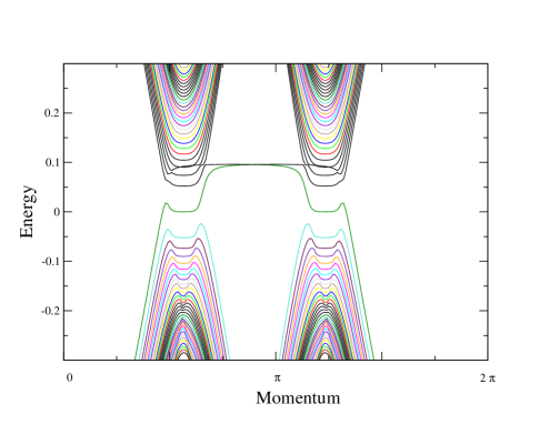
Figure 1: (color on line) Energy spectrum (in units of $t$) for a graphene ribbon $600a$ wide, as a function of the momentum $k$ along the ribbon (in units of $1/(\sqrt{3}a)$), with a magnetic flux of $5\times 10^{-4}\Phi_{0}$ per hexagon, in the presence of confining potential (see text).

At low energies and long wavelengths, the energy spectrum of Hamiltonian (1) reduces to two Dirac cones centered at the $K$ and $K^{\prime}$ points in the Brillouin zone. Around each Dirac point the Hamiltonian (1) can be written as:

$$H_{0}=\bm{\sigma}\cdot(v_{F}\bm{p}+e\bm{A})\,,$$ (2)

where $v_{F}=3ta/2$, $\bm{\sigma}$ are Pauli matrices acting on the states, $\psi({\bf r})=(\psi_{A}({\bf r}),\psi_{B}({\bf r}))$, of the two sub-lattices, and ${\bf p}=(p_{x},p_{y})=-i\bm{\nabla}$ is the 2D momentum operator. In the absence of confinement ($V(x)=0$) we can diagonalize (2) and one finds Landau levels given by:

$$E_{n,\sigma} = \sigma\sqrt{2}v_{F}\sqrt{n}\,\,/\ell_{B}=\sigma v_{F}\sqrt{2eB\,n}\,,$$ (3)

where $\ell_{B}=1/\sqrt{eB}$ is the cyclotron length, $n$ is a positive integer, and $\sigma=1$ $(-1)$ labels the electron (hole) levels.

As discussed in the context of neutrino billiards Berry and Mondragon (1987), the problem in the continuum suffers from the difficulty that in trying to confine massless Dirac particles in a region of size $L$ by including a large potential $V$ at the edge, leads to a situation where particles still exist even at energies higher than $V$. This problem, of course, does not arise in the tight-binding description. In order to avoid this problem in the continuum description, we introduce a position dependent mass term: $H_{c}=v_{F}^{2}M(x)\sigma_{z}\,,$ where,

$$M(x)=\left\{\begin{array}[]{c}M,\hskip 28.45274ptx<-L/2\,,\\ 0,\hskip 11.38092pt-L/2\leq x\leq L/2\,,\\ M,\hskip 28.45274ptx>L/2\,,\\ \end{array}\right.$$ (4)

where $L$ is the width of the graphene stripe. We are interested in the hard wall case ($M\to\infty$) although other potentials can be studied in analogous way nex . Notice that in the absence of an applied magnetic field, a mass term does not break particle-hole symmetry, as in the case of a potential $V(x)$)Berry and Mondragon (1987). Nevertheless, since both $V(x)$ and $M(x)$ are strongly concentrated at the edge (in a distance of the order of the lattice spacing), they do not modify the states in the bulk. It is also worth mentioning that although (2) is not time reversal symmetric in the absence of a magnetic field Berry and Mondragon (1987), time reversal is recovered by the inclusion of the second Dirac cone at the opposite side of the Brillouin zone.

The Dirac equation, $H\psi=E\psi$, where $H=H_{0}+H_{c}$, can be recast in terms of a wavefunction ansatz, $\phi=(H+E)\psi$, as: $H^{2}\phi=E^{2}\phi$. It is easy to show that this wavefunction has the form: $\phi(x,y)\propto e^{-iky}\varphi_{\sigma}(x)\,,$ where $k$ is the momentum along the $y$ direction, $\sigma=\pm 1$ are the eigenstates of $\sigma_{z}$, and $\varphi_{\sigma}(x)$ obeys the following equation:

$$\left[-\frac{\partial^{2}}{\partial\xi^{2}}+\xi^{2}+V(\xi)\right]\varphi_{\sigma}(\xi)=\epsilon\varphi_{\sigma}(\xi)\,$$ (5)

where,

$$\xi = x/\ell_{B}-k\ell_{B}\,,$$ (6)

$$V(\xi) = [v_{F}\ell_{B}M(\xi)]^{2}\,,$$ (7)

$$\epsilon = (\ell_{B}E_{\sigma}/v_{F})^{2}-\sigma\,.$$ (8)

Equation (5) is a dimensionless Schrödinger equation for a non-relativistic particle (of mass $1/2$) in a parabolic potential (of frequency $\omega_{0}=2$) superimposed to a potential well, $V(\xi)$, whose position shifts with the momentum $k$ (see Fig. 2). We see, from (8), that the Dirac fermion spectrum in the presence of the magnetic field and confining potential can be written as:

$$E_{\epsilon,\sigma}=\sigma v_{F}\sqrt{\epsilon+\sigma}/\ell_{B}\,.$$ (9)

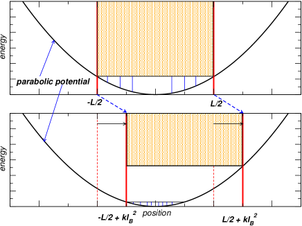
Figure 2: (color on line) Illustration of the potentials in the problem: $k=0$ (top) and $k\neq 0$ (bottom).

At low energies (small $\epsilon$) the parabolic potential dominates and the wavefunctions look like the ones in the infinite system ($L\to\infty$) in the presence of magnetic field Peres et al. (2006). In this limit, the spectrum of (5) is given by the 1D harmonic oscillator: $\epsilon\approx\omega_{0}(n+1/2)=2n+1$. This result, together with (9), gives rise to eq. (3), with the energy proportional to $\sqrt{B}$. On the other hand, at large energies, the confining potential becomes more important and the energy spectrum changes to: $\epsilon\approx[\pi n/(L/\ell_{B})]^{2}$, leading to a Dirac fermion spectrum of the form:

$$E_{n,\sigma}\approx\sigma v_{F}[\pi n/L+\sigma LeB/(2\pi n)]\,,$$ (10)

which leads to a spectrum proportional to $B$. These simple arguments show that the SdH magneto-resistance oscillations changes behavior as a function of magnetic field. On the one hand, for a given chemical potential $\mu$, eq. (3) predicts that the maxima of the SdH should happen at fields:

$$1/B_{F}(N,L)=(2v_{F}^{2}e/\mu^{2})\,N\,,$$ (11)

where $N$ is the Landau level index. On the other hand, eq. (10) shows that the maxima occur at fields:

$$1/B_{F}(N,L)=[L^{2}e/(2\pi^{2}N)]/(N_{c}(L)-N)\,,$$ (12)

where

$$N_{c}(L)=\mu L/(\pi v_{F})\,.$$ (13)

Hence, $1/B_{F}(N)$ diverges at a critical Landau level index $N_{c}(L)$ which increases linearly with the width $L$ of the graphene stripe. The deviation from (11) to (12) is a clear sign of the Dirac fermion confinement.

Figure 3: (color on line) Energy spectrum, $E_{\sigma}(k)$, as function of $k\ell_{B}^{2}/L$ for two system sizes, $L=50$ nm and $L=500$ nm, at $B=1$ T, for 10 eigenstates. Each Landau level is sub-divided into two sub-levels, distinguished be the quantum number $\sigma$.

Notice that the crossover from (3) to (10) (or from (11) and (12)) occurs when the Landau orbit fits into the confining potential. Since each orbit must enclose exactly an integer number of flux quantum, $\Phi_{0}$, the crossover occurs at a magnetic field $B^{*}$ such that, $B^{*}L^{2}\approx N\Phi_{0}$, that is,

$$B^{*}(N,L)=N\Phi_{0}/L^{2}\,.$$ (14)

Let us now consider the numerical solution of the differential equation (5) written in terms of the above introduced dimensionless variables in the case $M\rightarrow\infty$. Because our treatment of the Dirac equation leads to a second order differential equation, the appropriate boundary conditions for a sharp confining edge with a mass term is McCann and Fal’ko (2004): $\varphi_{\sigma}(-L/(2\ell_{B})+k\ell_{B})=\varphi_{\sigma}(L/(2\ell_{B})+k\ell_{B})=0$. In Fig. 3 we show the energy spectrum at $B=1$ T for two different system sizes as a function of $k\ell^{2}/L$. One can clearly see that the degeneracy of the Landau levels is lifted for small enough system sizes or large enough $k$ Brey and Fertig (2006); Abanin et al. (2006). For small $k$ the energy states are dispersionless and degenerate.

Figure 4: (color on line) Wave functions $\varphi_{\sigma}$ for $L=500$ nm. The values of the magnetic field are, from left to right and top to bottom, $B=$ 5, 2.5, 1.25, 0.6, 0.3, 0.1, 0.05, 0.025, 0.01 (T).

In Fig. 4 we show the first two state eigenvalues of the effective Schrödinger equation (5), for $k=0$ and different values of the field (or, equivalently, different system sizes). One can clearly observe the change in the wavefunction from cosine (sine) to gaussian (first order Hermite polynomial times gaussian) behavior as $l_{B}$ decreases. Clearly the system evolves from a state where the boundaries introduced by the confining potential are irrelevant (the wave functions and the energy levels are essentially those of the 1D harmonic oscillator at $B=5$ T, and $l_{B}\simeq$ 12 nm), passing to a state where the gaussian decay of the wave function in the classically forbidden regions is important allowing the electrons to feel the presence of the confinement potential (the wave functions and the energy levels cannot be described either by the 1D harmonic oscillator or by the particle in a box for $B=0.1$ T at $l_{B}\simeq$ 80 nm). Finally, when the Landau orbit is of the order of size of the confinement potential, the eigenstates are essentially those of the particle in a box ($B=0.01$ T, $l_{B}\simeq$ 250 nm).

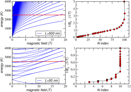
Figure 5: (color on line) Landau plots for two system sizes, $L$= 500, 50 nm. On the right hand side, we depict the energy levels (in K) as a function of magnetic field (in T) and the horizontal line marks the position of the Fermi energy. On the left hand size we plot $1/B_{F}(T)$ as a function of the Landau index $N$.

In Fig. 5, we show the energy spectrum as a function of the magnetic field for different system sizes together with their respective Landau plots. Note that at small fields (when $L$ is large enough) the energy spectrum follows the $\sqrt{B}$ dependence of (3) while at larger fields it becomes linear in $B$ as predicted by (10). The crossover from these two asymptotic behaviors is indeed given by eq. (14), as one can see from the size dependence. More striking, however, is that fact that $1/B_{F}$ indeed diverges at sufficiently high Landau level index and that the size dependence is given by (13).

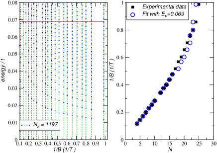
Figure 6: (color on line) On the left hand side, we show the energy spectrum (in units of $t$) as a function of $B^{-1}$ (in T^-1). The horizontal line shows position of the Fermi energy ($\approx 0.069t$). On the right hand side, we show the theoretical Landau plot (open circles) in comparison with the experiments of ref. [Berger et al., 2006] (close squares).

In Fig. 6 we compare our tight binding results with with the experimental data of ref. [Berger et al., 2006]. We choose a ribbon of size $295$ nm (equivalent to $N_{c}=1197$ unit cells), and Fermi energy $0.069t$ (equivalent to $0.22$ eV). Notice the excellent agreement between theory and experiment for $N<16$ ($2{\rm T}<B<10{\rm T}$). For $N>16$ there is shift of $N$ by one (either plus or minus one) relative to the experiment. This discrepancy, we believe, can be assigned to the experimental difficulty in assigning the Landau indices at small magnetic fields Berger et al. (2006).

In summary, we have studied the problem of Dirac confinement in graphene, that is, graphene’s zitterbewegung, for graphene stripes of size $L$ in the presence of a transverse magnetic field, $B$. We show that the interplay between size effects and magnetic field can be studied in the continuum limit using the Dirac equation coupled to a vector potential. We present arguments that show that the spectrum of the problem shows a crossover from magnetic field dominated to confinement dominated as a function of magnetic field or system size. The crossover occurs when the radius of the Landau level becomes of the order of the width of the system. In the crossover the spectrum changes from $\sqrt{B}$ to linear in $B$ and that the Landau plots, that can be measured in a SdH experiment, change from dramatically in the presence of a finite system. Our results are in excellent agreement with experiments.

We are very grateful to C. Berger and W. A. de Heer for providing the experimental data. A.H.C.N. was supported through NSF grant DMR-0343790. N. M. R. P. thanks ESF Science Programme INSTANS 2005-2010, and FCT under the grant POCTI/FIS/58133/2004. F. G. acknowledges funding from MEC (Spain) through grant FIS2005-05478-C02-01.

References

- Novoselov et al. (2004) K. S. Novoselov et al., Science 306, 666 (2004).
- Novoselov et al. (2005a) K. S. Novoselov et al., Proc. Nat. Acad. Sc. 102, 10451 (2005a).
- Novoselov et al. (2005b) K. S. Novoselov et al., Nature 438, 197 (2005b).
- Zhang et al. (2005a) Y. Zhang et al., Nature 438, 201 (2005a).
- Pereira et al. (2006) V. M. Pereira et al., Phys. Rev. Lett. 96, 036801 (2006).
- Peres et al. (2006) N. M. R. Peres et al., Phys. Rev. B 73, 125411 (2006).
- Kane and Mele (2005) C. Kane and E. J. Mele, Phys.Rev.Lett. 95, 146802 (2005).
- Berger et al. (2004) C. Berger et al., J. Phys. Chem. B 108, 19912 (2004).
- Zhang et al. (2005b) Y. Zhang et al., Phys. Rev. Lett. 94, 176803 (2005b).
- Peres et al. (2005) N. M. R. Peres et al. (2005), eprint cond-mat/0512476.
- Itzykson and Zuber (1980) C. Itzykson and J. Zuber, Quantum Field Theory (McGraw-Hill, 1980).
- Beenakker and van Houten (1991) C. W. J. Beenakker and H. van Houten, Quantum transport in semiconductor nanostructures, vol. 44 (Academic Press, New York, 1991), eprint cond-mat/0412664.
- (13) N. M. R. Peres et al., unpublished.
- Berry and Mondragon (1987) M. V. Berry and R. J. Mondragon, Proc. R. Soc. Lond. A 412, 53 (1987).
- McCann and Fal’ko (2004) E. McCann and V. I. Fal’ko, J. Phys.: Condens. Matter 16, 2371 (2004).
- Abanin et al. (2006) D. A. Abanin et al. (2006), eprint cond-mat/0602645.
- Brey and Fertig (2006) L. Brey and H. Fertig (2006), eprint cond-mat/0603107.
- Berger et al. (2006) C. Berger et al., to appear on Science (2006).