Optimized multicanonical simulations: a new proposal based on classical fluctuation theory

Abstract

We propose a new recursive procedure to estimate the microcanonical density of states in multicanonical Monte Carlo simulations which relies only on measurements of moments of the energy distribution, avoiding entirely the need for energy histograms. This method yields directly a piecewise analytical approximation to the microcanonical inverse temperature, $\beta(E)$, and allows improved control over the statistics and efficiency of the simulations. We demonstrate its utility in connection with recently proposed schemes for improving the efficiency of multicanonical sampling, either with adjustment of the asymptotic energy distribution or with the replacement of single spin flip dynamics with collective updates.

I Introduction

Over the past decade, the use of Monte Carlo methods Newman and Barkema (1999) has broken the boundaries of statistical physics and has become a widely used computational tool in fields as diverse as chemistry, biology and even sociology or finance.

Despite the enormous success of the well known Metropolis importance sampling algorithm, its narrow exploration of the phase space and characteristic convergence difficulties motivated a number of different approaches. Firstly, the techniques for harvesting useful information from the statistical data obtained at a given temperature were improved in order to extrapolate the results in a small temperature range and, therefore, reduce the number of required independent simulations Ferrenberg and Swendsen (1988, 1989). Secondly, cluster update algorithms were proposed Niedermayer (1988); Wolff (1989); Swendsen and Wang (1987) in order to overcome critical slowing down. Finally, the requirement of constant temperature was lifted, allowing the system to explore a wider range of the energy spectrum. In Simulated Tempering, the temperature becomes a dynamical variable, which can change in the Markov process Marinari and Parisi (1992); Parallel Tempering uses several replicas of the system running at different temperatures and introduces the swapping of configurations between the various Markov chains Hukushima and Nemoto (1996); Tesi et al. (1996); Hagura et al. (1998). The flat histogram approach Berg and Celik (1992); Lee (1993) replaces the asymptotic Boltzmann distribution for the asymptotic probability of sampling a given state of energy $E_{i}$, $p_{i}\propto\exp(\beta E_{i})$, by $p_{i}\propto 1/n(E)$, $n(E)$ being the microcanonical density of states, thus ensuring that every energy is sampled with equal probability.

The first major obstacle to this last approach is the obvious difficulty of accessing the true density of states of a given system; several clever algorithms have been proposed to this end Berg and Celik (1992); Wang and Landau (2001a). Nevertheless, even in cases where the true density of states is known a priori, recent studies Dayal et al. (2004); Costa et al. (2005) have shown that very long equilibration times can remain a serious concern with multicanonical methods. Furthermore, the number of independent samples is strongly dependent on energy, making error estimation rather tricky Viana Lopes and Lopes Dos Santos . This has led some authors (Marinari et al. (2001)) to question the reliability of the results obtained by the Multicanonical Method in spin glass models at low temperatures. To address these issues, the requirement of a perfectly flat histogram was also lifted Trebst et al. (2004), sacrificing the equal probability of sampling each energy in favor of minimizing tunneling times.

In section II, we propose a variation of the algorithm to estimate the density of states that does not use histograms, instead relying entirely of measurements of cumulants of the energy distribution at each stage of the simulation to build a piecewise analytical approximation to the statistical entropy, $S(E)=\ln\left(n(E)\right)$, and inverse temperature $\beta(E)=dS(E)/dE$. We find that the time required to explore the entire energy spectrum scales more favorably with system size than histogram based methods. The method is as easy to apply in systems with continuous spectrum as in the discrete case, can be quite naturally adapted to running a simulation in a chosen energy range, and accommodates without difficulty tunneling times optimization schemes and cluster update methods.

In Section III we show that the optimization scheme proposed in Trebst et al. (2004) can be applied during the process of estimating the density of states, still avoiding histograms, and with significant efficiency gains.

In Section IV, we demonstrate the usefulness of the analytical approximation of $\beta(E)$ in generalizing Wolff’s cluster algorithm Wolff (1989) to multicanonical simulations. This generalization maintains an acceptance probability still very close to unity, growing large clusters at low temperatures and small ones at higher temperatures. The optimization procedure reported in Trebst et al. (2004) is also implemented for this cluster dynamics.

This algorithm has already been applied with success to both discrete (Ising models on regular lattices and Small World networks, Ising Spin Glasses)Viana Lopes et al. (2004) and continuous models (XY and Heisenberg models, with both short and long-range interactions, namely dipolar interactions)Costa (2001), but this is its first systematic presentation.

II Proposal

The usual way of ensuring an asymptotic distribution $p_{i}\propto\exp\left[-\omega(E_{i})\right]$ is to use a Markov chain algorithm in which the transition probability to go from state $i$ to state $j$ with respective energies $E_{i}$ and $E_{j}$ is

$$W_{ij}=\min(1,e^{-\Delta\omega(E)}).$$ (1)

This choice leads to an asymptotic energy distribution probability given by

$$H(E)\propto\exp(S(E)-\omega(E)),$$ (2)

where the entropy is defined as the logarithm of the (unknown) density of energy states, $S(E)=\ln\left(n(E)\right)$. In principle, this relation allows a calculation of the entropy $S(E)$ (up to an irrelevant constant $S_{0}$) from a numerical determination of the distribution $H(E)$ for any value of the energy $E$ simply as:

$$S(E)=S_{0}+\omega(E)+\ln H(E)$$ (3)

However, this is not always efficient for any choice of the function $\omega(E)$. Consider, for example, the widely used Metropolis choice, $\omega(E)=\beta E$ (with $\beta=1/T$, the inverse temperature). In many systems, the resulting distribution $H(E)$ has the shape of a bell curve, usually approximated by a Gaussian distribution (Figure 1). Since it is very unlikely to generate statistically significant configurations in the tails of the distribution for $H(E)$, the usefulness of the formula (3) is limited to values of $E$ not too far from the mean value $\mu_{\beta}$. “Not too far” means explicitly that the above formula is limited to those values of $E$ such that $|E-\mu_{\beta}|<\alpha\sigma_{\beta}$ with $\alpha\sim 2-4$. The mean value $\mu_{\beta}$ and the variance $\sigma_{\beta}^{2}$ of the distribution $H(E)$ satisfy:

$$\left.\frac{dS}{dE}\right|_{\mu_{\beta}}=\beta;\hskip 14.22636pt\left.\frac{d^{2}S}{dE^{2}}\right|_{\mu_{\beta}}=-\frac{1}{\sigma_{\beta}^{2}}$$ (4)

A clever choice for $\omega(E)$ can greatly improve the range of values of $E$ for which the formula (3) is useful. For instance, if we were to chose $\omega(E)\propto\ln(n(E))$ then the resulting distribution $H(E)$ would be constant in $E$ and all the energy values would be sampled with the same frequency. However, it is clear that this is impossible since $n(E)$ is precisely the function we want to determine.

Berg’s scheme uses a series of functions $\omega_{i}(E)$, each one of them gives information on $n(E)$ for a range of energy values. The initial choice $\omega_{0}(E)=0$ (equivalent to a Metropolis choice at infinite temperature) provides a histogram $H_{0}(E)$ from which one derives an estimation of the entropy, $S_{0}(E)$, valid for those values of $E$ visited in a statistically significant way. After this stage, a new simulation is performed with $\omega_{1}(E)=S_{0}(E)$ in the region visited in the previous simulation, from which we obtain an entropy estimate $S_{1}(E)$ valid in another range of energies, and so on. Berg proposes a recursion scheme that allows systematic corrections of $\omega_{i}(E)$ at all visited energies, and ensures the convergence to the true entropy for any energy, so ensuring a flat energy histogram.

Figure 1: Schematic representation of the true derivative of the entropy $S(E)$ and two different choices for the derivative of $\omega(E)$, with the corresponding energy probability distributions. In panel a), the Metropolis approach, where $\omega(E)=\beta E$ and, in panel b), the ideal extended ensemble approach with $\omega(E)=S(E)$.

This procedure has some limitations. To begin with, the entropy can only be estimated inside the energy range visited in the last simulation and a bad choice for the entropy outside this region can severely limit the exploration of lower energies; secondly, rarely visited energies introduce a large error in the estimated entropy (hence the need for recursion introduced by Berg in order to minimize this error). Furthermore, the fact that one counts visits in each energy implies that, for continuous systems, the energy spectrum must be discretized.

Thermodynamic functions such as the entropy can be treated as continuous functions of energy, both for discrete and continuous spectra, for not too small systems. We make use of the Gaussian approximation:

$$S(E)\approx S(\mu_{\beta})+\beta(E-\mu_{\beta})-\frac{1}{2\sigma_{\beta}^{2}}(E-\mu_{\beta})^{2}$$ (5)

to propose the sequence of weight functions $\omega(E)$.

Figure 2: In the current proposal, the weight function $\omega(E)$ approximates the entropy between two energies $\mu_{r}$ and $\mu_{0}$ and is linear in energy outside this region, $d\omega/dE=\beta_{r}$ for $E<\mu_{r}$ and $d\omega/dE=\beta_{0}$ for $E>\mu_{0}$.

After running an initial simulation at a inverse temperature $\beta_{0}$, with $\omega_{0}=\beta_{0}E$, and measuring $\mu_{0}$ and $\sigma_{0}$, we modify the weight function to $\omega_{1}(E)$ defined by:

$$\frac{d\omega_{1}(E)}{dE}=\left\{\begin{array}[]{ccc}\beta_{0}&&E>\mu_{0}\\ \beta_{0}-\frac{1}{\sigma_{0}^{2}}(E-\mu_{0})&&\mu_{1}<E<\mu_{0}\\ \beta_{1}&&E<\mu_{1}\end{array}\right.$$ (6)

with $\mu_{1}=\mu_{0}-\alpha\sigma_{0}$ and $\beta_{1}=\beta_{0}+\alpha/\sigma_{0}$. In a new simulation with transition rates $W_{ij}=\min(1,e^{-\Delta\omega_{1}(E)})$ we obtain $H(E)\simeq\texttt{constant}$, for energies such that $\mu_{1}<E<\mu_{0}$, while for $E<\mu_{1}$, $H(E)$ is a “half Gaussian” with maximum at $\mu_{1}$. It is straightforward to estimate $\sigma_{1}$ from the average of $\left(E-\mu_{1}\right)^{2}$ for $E<\mu_{1}$. We are therefore be able to add another branch to $\omega(E)$, and so on, until we reach the lowest temperature we wish to study. On the iteration of order $r$ the histogram is flat between $\mu_{0}$ and $\mu_{r}$ and half Gaussian below $\mu_{r}$ (Figure 2). Using $\omega(E)=\beta_{0}$ for $E>\mu_{0}$, we effectively restrict the simulation to energies below $\mu_{0}$, apart from a Gaussian tail above this energy.

The fact that $\beta(E)=\texttt{const}$ in the unexplored energy regions, corresponding to Boltzmann sampling, means that we can use all techniques developed for the Metropolis algorithm in order to be confident on the results obtained in this region, before moving on to lower energies. These regions of canonical sampling can also be used to restrict the simulation to a specific temperature range, for instance around a critical temperature, which can dramatically increase the efficiency and precision of the simulation. The method can also be refined by keeping higher order terms in the expansion of the entropy which can be obtained by measuring higher order moments of the energy. We have successfully used an expansion of $S(E)$ up to fourth order terms.

II.1 Comparison with histogram based recursion

We compared an implementation of this proposal based on classical fluctuation theory (CFP) with the multicanonical recursion as described in Berg (2003) in a simulation of a two dimensional Ising model:

$$H=-J\sum_{<ij>}s_{i}s_{j}.$$

Except for the method of estimating the density of states (or rather, its logarithm, the entropy), the results were obtained using exactly the same code, specifically with the same number of steps per run. We chose the number of Monte Carlo steps (MCS) in each iteration (run) to increase linearly with the iteration number, $r$, specifically as $r\times 10^{5}\,\texttt{MCS}$. This is a rather arbitrary choice which is necessary for comparison purposes. In fact, our proposal allows us to set the number of steps in the yet unexplored energy region as the criteria for moving on to the next run, which, in turn, allows better statistical control over the next estimate for the entropy. For a fair comparison between the two algorithms we choose $\beta_{0}=0$ for CFP and impose $\beta(E)=0$ in the histogram based method for $E>\mu_{0}$. In this way the algorithms only explore the positive temperature region of the spectra.

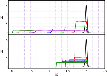
Figure 3: A comparison of the evolution of the multicanonical recursion in the present scheme (upper panel) and the one described in Berg (2003) (lower panel). The simulation was done for a Ising square sample with $L=64$, and, for simplicity, we only show histograms from 1 out of each 5 runs.

Figure 3 shows 7 histograms out of 35 runs of simulations on a $64\times 64$ Ising model, with $r\times 10^{5}\texttt{\, MCS}$ per run, which was enough to reach the ground state with our algorithm. Several more runs are required using an histogram based method (lower panel of fig. 3). It is important to note that the full range of visited energies, $\sim\left(\mu_{0}-\mu_{r}\right)$, does not increase linearly with run number, $r,$ because the spectral range added in each run shrinks as one approaches the ground state. In this respect the difference in performance of the two methods is quite remarkable. Histogram based methods do not provide an estimate for the entropy outside the previously visited energy range. As a result, for energies in the previously unvisited range, $H(E)$ decays as

$$H(E)\sim\exp\left[S(E)\right]\sim\exp\left[-\beta_{r}(E_{r}-E)\right]$$

where $E_{r}$ is the lowest energy of the previous run and $\beta_{r}=\beta(E_{r}).$ Our method uses $\omega(E)=\beta_{r}E$ which leaves

$$H(E)\sim\exp\left[S(E)-\omega(E)\right]\sim\exp\left[-\frac{1}{2\sigma_{r}^{2}}(E_{r}-E)^{2}\right]$$

Since $\sigma_{r}^{2}$ scales linearly with $N$, the added energy range in each iteration scales differently in the two methods. In terms of energy per particle, the added energy range per run, $\Delta\epsilon=\Delta E/N$, scales as $1/L=N^{-1/2}$ in the current proposal instead of $\left(\beta_{r}N\right)^{-1}$ in histogram based methods. In Figure 4 we plot the visited energy per particle range after $r$ iterations, for various system sizes, as a function of $r/L$ for the CFP method and $r/N$ for histogram based method. The collapse of the curves for the various systems sizes shows that the number of runs required to cover the same energy per particle range scales with with $L=\sqrt{N}$ in the current proposal (left panel) and $N$ in histogram based methods (right panel).

Figure 4: Full range of visited energies ($E_{r}-E_{0})/N$, as a function of the system size and number of iterations, $r$, for current method (left panel) and for histogram based recursion (right panel); in our moment based method $r$ scales $L=\sqrt{N}$ whereas, with histograms, it scales with $N$.

The two methods perform similarly for small systems, but the advantage of CFP method becomes obvious for large $N$ and no amount of fine tuning can disguise it.

Nevertheless, other alternative schemes to Berg’s recursion have already been proposed like Wang-Landau sampling Wang and Landau (2001b) or the transition matrix method Wang et al. (1999). As will be seen shortly, the main advantage of our method is that, unlike these previous methods, it produces an analytic approximation to the microcanonical inverse temperature, $\beta(E)$, in an increasing energy range, right from the start of the simulation. That proves an asset in the implementation of procedures designed to overcome the slow down with system size that affects multicanonical simulations Dayal et al. (2004); Trebst et al. (2004); Wu et al. (2005).

III Optimization of tunneling times

In a recent publication, Trebst, Huse and Troyer showed that it is possible to decrease significantly the tunneling times of a multicanonical simulation, by abandoning the requirement of a flat histogram Trebst et al. (2004). Our procedure of construction of the statistical entropy is well suited to implement their optimization method, right from the start of the simulation, without having to construct an approximation to $n(E)$ for the entire spectrum.

The procedure proposed in Trebst et al. (2004) minimizes the average time required to span the gap between two fixed energies in the spectrum, $E_{-}$ and $E_{+}$.

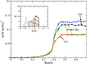
Figure 5: Tunneling time (scaled by $(N\log N))^{2}$, for system sizes $N=48\times 48$ and $N=64\times 64$, as an function of the recursion run divided by $L$ which is proportional to the energy per particle range. (a) CFP without optimization; (b) for an application of the optimization procedure only after an estimation of density of states in the chosen range of temperatures; (c) our implementation of the optimization. The inset shows the histograms obtained for the sample with $L=64$ in several runs during the exploration of the energy spectrum with optimization.

To achieve this purpose, one must distinguish each energy entry during the simulation according to which of the two energies, $E_{-}$ or $E_{+}$, was visited last. We can thus measure separately $n_{-}(E)$, the number of visits to energy $E$ occurring when the simulation has visited $E_{-}$ more recently than $E_{+}$, and $n_{+}(E)$ for the other way around. To minimize the tunneling times between the two energies $E_{-}$ and $E_{+}$ one must choose an asymptotic energy distribution that satisfies

$$H(E)\propto\frac{df(E)}{dE}$$ (7)

where $f(E)=n_{+}(E)/H(E)$. The implementation proposed in Trebst et al. (2004) used the knowledge of the density of states, $n(E)$ in the whole spectrum to measure the $f(E)$, following with a recursion procedure that converges to the asymptotic distribution which satisfies eq. 7. In our method of construction of the density of states there are, at each step, two energies which are the current boundaries of the known density states, namely $\mu_{0}$ (that remains fixed) and $\mu_{r}$ (that changes with each run, $r$). Therefore, by using $E_{-}=\mu_{r}$ and $E_{+}=\mu_{0}$ we can measure $f(E)$. In the first run, for $\mu_{1}<E_{i}<\mu_{0}$, we observe $H_{1}(E_{i})\propto\exp\left(-\omega_{1}(E)\right)$, with $\omega_{1}(E)$ defined in eq. 6, rather than the optimal distribution $H^{opt}(E)\propto\exp\left[\ln\left(df_{1}/dE\right)\right]$. To converge to the optimal distribution (changing the weight alters $f(E)$), we use, in the next run, the geometric mean $\sqrt{H_{1}H^{opt}}$ in the interval $\mu_{1}\leq E\leq\mu_{0}$ Trebst et al. (2004): the weight factor becomes $-\omega_{2}(E)+\phi_{2}(E)$, where

$$\phi_{2}(E)=\frac{1}{2}\ln\left(\frac{df_{1}}{dE}\right)\qquad\mbox{for }\mu_{1}\leq E\leq\mu_{0},$$

with constant values of $\phi_{2}(\mu_{1})$ for $E<\mu_{1}$ and $\phi_{2}(\mu_{0})$ for $E>\mu_{0}$. Notice that the correction to the microcanonical temperature, $\beta(E)$, is $-d\phi_{2}(E)/dE$ which is zero for $E<\mu_{1}$. This choice ensures the convergence to the criterion of eq. 7 in the range where the entropy is already known and where $f(E)$ was measured, $\mu_{1}<E<\mu_{0}$, and gives a flat histogram in the region where the entropy was estimated by calculating moments of the Gaussian tail, i.e. $\mu_{2}<E<\mu_{1}$. This procedure is iterated in the following runs with $\phi_{r}(E)$ defined as,

$$\phi_{r}(E)=\frac{1}{2}\left[\phi_{r-1}+\ln\left(\frac{df_{r-1}}{dE}\right)\right];\qquad\mu_{r-1}\leq E\leq\mu_{0}$$

with constant values $\phi_{r}(\mu_{r-1})$ for $E<\mu_{r-1}$ and $\phi_{r}(\mu_{0})$ for $E>\mu_{0}$. To extract the numerical derivative of $f(E)$, avoiding the difficulties of the fluctuations in histogram entries, we use the natural scale afforded by $\sigma_{\beta}$, and calculate $df/E$ as

$$\left.\frac{df}{dE}\right|_{\mu_{\beta}}=\frac{\left\langle f(E)\left(E-\mu_{\beta}\right)\right\rangle_{\beta}}{\sigma_{\beta}^{2}}.$$

In figure 5 we plot the average tunneling time, divided by $(N\ln N)^{2}$, for two different system sizes, as an function of the run number of the multicanonical recursion divided by $L=\sqrt{N}$; simulations with the same horizontal coordinate correspond to the same energy per particle range. Curves (a) correspond to the situation without optimization, and the average tunneling times vary faster than $(N\ln N)^{2}$; the two sizes do not collapse to a single curve. In case (c), with the optimization carried out while the density of states is being determined, the curves for the two system sizes track each other. If the optimization correction is only performed after full exploration of the energy spectrum, curve (b), there is no further gain in tunneling time, as the average tunneling times of (b) merge with curve (c). This observation clearly supports our suggestion that optimization can be implemented while the density of states is being constructed. In this fashion, it not only reduces tunneling times when $n(E)$ is known, but also speeds up the actual calculation of $n(E)$. As found in Trebst et al. (2004), the inset shows a strong signature of the optimizing procedure in the critical energy where the diffusivity is low.

IV Cluster Dynamics

An alternative way to improve the efficiency of multicanonical simulations consists in changing the specific dynamics of the Markov chain, i.e., the algorithms used to propose and accept configuration moves.

In canonical ensemble simulations, cluster update algorithms like Wolff’s Wolff (1989), Swendsen-Wang Swendsen and Wang (1987) or Niedermeyer’s Niedermayer (1988) have proved very effective in overcoming critical slowing down of correlations. Several proposals have been presented to generalize cluster update approaches in multicanonical ensemble simulations, either using spin-bond representations of the partition function, Janke and Kappler (1995a, b); Yamaguchi and Kawashima (2002); Wu et al. (2005), or cluster building algorithms based on alternative ways of computing the microcanonical temperature, $\beta(E)$ Reynal and Diep (2005a, b).

Wolff’s cluster algorithm Wolff (1989) provides a clever way of growing a cluster of parallel spins which can be flipped with probability 1, and still maintain the required Boltzmann asymptotic distribution. This remarkable possibility is intimately related to the fact that $\omega(E)$ is linear in energy, $\omega(E)=\beta E$, in a Metropolis simulation.

In a multicanonical simulation, each step of the corresponding Markov chain occurs with the same probability as that of a canonical ensemble simulation, with an effective temperature $\beta_{i}$ chosen as $\beta_{i}=\beta(E_{i})$, $E_{i}$ being the energy of the current configuration; hence the designation “Multicanonical”. With this in mind, the simplest way of implementing cluster dynamics in a multicanonical simulation is to use $\beta_{i}=\beta(E_{i})$ to grow a cluster exactly as proposed in Wolff’s algorithm. However, since the reverse path implies a different value of $\beta$, $\beta_{j}=\beta(E_{j})$, where $E_{j}$ is the energy of the next configuration in the chain, we must include an acceptance probability to ensure detailed balance.

In figure 6 we illustrate a move involving the flipping of four spins (labelled $1$ to $4$) on the left, and the reverse move on the right. The site marked with the number 1 has been chosen with uniform probability. If a bond connects spin 1 to a neighboring spin parallel to 1 it is added to the cluster with a probability $p_{i}$ and rejected with probability $1-p_{i}$. This step is then repeated for the neighbours of the initial spin which were added to the cluster, until the process stops and there are no further bonds that can be aggregated to the cluster. The probability of generating a cluster with $n_{a}$ accepted bonds, in which $n_{r}$ bonds to spins parallel to the initial one were inspected and rejected, is given by:

$$G_{i\to f}=p_{i}^{n_{a}}(1-p_{i})^{n_{r}}.$$

It is important to note that $n_{r}$ includes a number of rejected bonds that now link spins inside the cluster (like the bond from spin $1$ to spin $4$ in fig. 6). We write $n_{r}=n_{p}+n_{f}$, where $n_{p}$ counts the number of such bonds and $n_{f}$ is the number of bonds from spins in the cluster to parallel spins outside the cluster. This distinction is important when considering the reverse move.

The difference in energy between the final and initial configuration is determined only by the frontier of the cluster; it is given as $\Delta E=-2J(n_{d}-n_{f})$ where $n_{d}$ is the number of bonds to spins opposite to the spins in the cluster. Let us now consider the reverse move, which requires us to select the same cluster in the same order with the spins now reversed we respect to the original state.

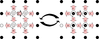
Figure 6: This scheme shows, on the left, how, starting from a given spin (marked as $1$), the bonds to neighbouring spins are inspected and marked according to the algorithm. On the right, are shown the resulting configuration and the way the initial state can be reached from it.

Referring once again to figure 6, one can see that the $n_{a}$ bonds that were accepted in the direct move (left) with probability $p_{i}$ must be accepted in the reverse move (right), each with probability $p_{j}$; the $n_{d}$ bonds to opposite spins in the direct move now connect to spins parallel to those in the cluster and must be rejected probability $(1-p_{j})$; the bonds to spins that were rejected in the direct move ($n_{f}$) are, in the reverse process, bonds to opposite spins and are, hence, rejected with probability $1$; finally the $n_{p}$ bonds that were rejected but link spins inside the cluster, must now also be rejected. In other words, for the direct move

$$G_{i\to f}=p_{i}^{n_{a}}(1-p_{i})^{n_{f}}(1-p_{i})^{n_{p}}$$ (8)

while, for the reverse process,

$$G_{f\to i}=p_{j}^{n_{a}}(1-p_{j})^{n_{d}}(1-p_{j})^{n_{p}}.$$ (9)

Wolff’s algorithm corresponds to choosing $p_{i}=p_{j}=1-\exp(-2J\beta)$ which implies that

$$\frac{G_{f\to i}}{G_{i\to f}}=(1-p_{i})^{n_{d}-n_{f}}=e^{\beta\Delta E}.$$

The detailed balance condition for Boltzmann’s equilibrium distribution is obtained for an acceptance probability of 1 for flipping the cluster. To ensure an asymptotic distribution proportional to $\exp\left[-S\left(E\right)\right],$ the detailed balance requires an acceptance probability given by

$$A_{i\to f}=\min\left(1,\frac{G_{f\to i}}{G_{i\to f}}e^{-\Delta S(E)}\right).$$ (10)

If we choose $p_{i}=1-e^{-2\beta_{i}J}$ where $\beta_{i}=\beta(E_{i})$, we find that this acceptance probability remains close to $1$ for most of the energy range (see fig.  7), falling only at very low temperatures. This behaviour is in strong contrast with the one for single spin flip dynamics, where the acceptance rate is only $1$ at the maximum of the density of states. If the inverse temperatures of the initial and final states are close, $\beta_{i}\approx\beta_{j}$, the acceptance rate becomes

$$A_{i\to f} \approx \min\left(1,\left(1-p_{i}\right)^{n_{f}-n_{d}}e^{-\Delta S(E)}\right)$$ (11)

$$= \min\left(1,e^{\beta_{i}\Delta E}e^{-\Delta S(E)}\right)$$ (12)

where we used $\Delta E=-2J(n_{d}-n_{f})$ to obtain the second expression. For small energy differences, $\Delta S\approx\beta_{i}\Delta E$ and the acceptance rate becomes close to unity.

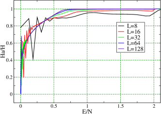
Figure 7: Acceptance ratio of the Wolff ’s cluster algorithm, with a microcanonical $\beta(E)$, for the 2D ferromagnetic Ising model. In the paramagnetic phase the acceptance ratio grows to $1$ with the increase of system size; in the ferromagnetic phase the acceptance ratio tends to a finite value, smaller than $1$, as $N$ grows.

In the case of the 2D ferromagnetic Ising model, the average excitation energy, $\Delta E$, is of $O(\sqrt{N})$ for energies below $\mu_{c}$ ($\mu_{c}=\mu_{\beta_{c}}$ where $\beta_{c}$ is the inverse critical temperature), of $O(1)$ for energies above $\mu_{c}$, with a crossover between these regimes in the neighborhood of $\mu_{c}$ (fig. 8). This behaviour reflects a huge difference with respect to single spin flip dynamics (SSF), where $\Delta E$ is always of $O(1)$. A similar behaviour exists for the number of spins, $n_{v}$ that are inspected in each call of the Markov chain: $n_{v}\sim O(1)$ for $E>\mu_{c}$ and $n_{v}\sim O(N)$ for $E<\mu_{c}$.

Figure 8: Two regime behavior of the Wolff’s cluster algorithm for the 2D ferromagnetic Ising model, with a microcanonical temperature $\beta(E)$. The left panel represents the equal energy average of the fraction of visited spins, $n_{v}$, during the cluster growing. In the ferromagnetic phase the number of visited spins is of the order of $O(N)$ and in the paramagnetic phase is of $O(1)$. The right panel it is represents the equal energy average of the excitations, $\Delta E$. In the paramagnetic phase $\sqrt{\left\langle\Delta E^{2}\right\rangle}$ becomes independent of the system size, while in the ferromagnetic phase it scales as $\sqrt{N}$.

This two regime behaviour introduces an additional complexity in this method. In particular, the tunneling time measured in Markov chains calls, no longer scales as the computational time with system size, since Markov chain calls can take a computational time of order $O(N)$. We therefore redefine the time scale so that a Markov chain call in a state of energy $E$ corresponds to a time span of $n_{v}(E)$, the average number of inspected spins in the cluster buildup process.

We now consider the system’s coarse grained random walk in energy space. When the energy is close to $E$, the mean square energy change in $M$ Markov chain calls is

$$\left\langle\Delta E^{2}\right\rangle_{M}=\left\langle\Delta E^{2}\right\rangle\times M$$

and this occurs in a time $\tau_{M}=M\times n_{v}(E)$. With time measured in this way, the diffusivity of this random walk in energy space is

$$D(E)\propto\frac{\left\langle\Delta E^{2}\right\rangle}{n_{v}(E)}.$$ (13)

On the other hand, the probability that the system is at energy $E$ is proportional to

$$H_{v}(E)=H(E)\times n_{v}(E),$$ (14)

since each visit to energy $E$ lasts a time $n_{v}(E)$. The probability current is given, quite generally, by

$$j=\rho(E)V(E)-\frac{d}{dE}\left(D(E)\rho(E)\right)$$

where, in equilibrium, $j=0$, and

$$\rho(E)=\rho_{0}(E)\equiv\frac{H_{v}(E)}{\int dEH_{v}(E)}.$$

$V(E)$ is a bias field, in general non-zero, which, together with $D(E)$, determines the equilibrium distribution.

It can be shown J. Penedones et al. (2006); Trebst et al. (2004) that the tunneling times of a random walk with a given diffusivity, $D(E)$, can be minimized with an optimal choice of bias field $V(E)$. The corresponding equilibrium distribution is given by

$$\rho_{0}(E)=\frac{1}{\sqrt{D(E)}}.$$

Using equations 13 and 14, this condition becomes

$$H(E)\propto\frac{1}{\sqrt{\left\langle\Delta E^{2}\right\rangle n_{v}(E)}}$$ (15)

This variation of $\log\left(H(E)\right)$, relative to a flat histogram, is of order $O(\log(N))$, and, therefore, histograms remain broad, covering the entire spectrum, but are no longer flat as shown in panel (a) of figure 9. On panel (d) it is shown that the tunneling time for this simulation scales has $N^{2}$ as expected from a simple diffusion.

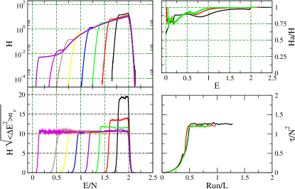
Figure 9: Results of the CFP recursion to construct an histogram given by eq. 15. (a) Histogram of the simulation for several steps of the CFP recursion; (b) Acceptance ratio; (c) ($H(E)\times\sqrt{n_{v}(E)\left\langle\Delta E^{2}\right\rangle}$) ; (d) Tunneling time (scaled by $N^{2}$) versus the run of the recursion (scaled by $L$).

The optimization procedure presented in reference Trebst et al. (2004), in the context of N-fold Way dynamics, is closely related to this one (but not identical) and leads to a choice

$$H(E)\propto\frac{1}{n_{v}(E)}\frac{df}{dE}$$

where $f(E)$ was defined above. We find only a marginal improvement in tunneling times with respect to the case of a histogram defined by eq. 15. These two procedures will be compared in another publication J. Penedones et al. (2006).

V Conclusion

We have proposed a new method to build the density of states in an multicanonical simulation. The method is based on the calculation of moments of the energy distribution. It avoids the use of histograms and can just as easily be implemented for continuous as for discrete systems. It leads to a piecewise analytic approximation to the microcanonical inverse temperature $\beta(E)$. In any stage of the simulation there are two well defined energies, $E_{-}$ and $E_{+}$, that limit the range in which $\beta(E)$ is known. Therefore the method can be applied without difficulty to a predefined temperature range such as a neighborhood of a critical temperature.

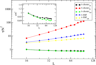
Figure 10: Scaling of tunneling time with system size in various broad histogram methods: (SSF) straight forward multicanonical simulation with single spin flip dynamics; ( SSF_opt) optimized single spin flip dynamics; $(\textrm{cluster}_{ob}$) optimized bias for the measured $D(E)$; ($\textrm{cluster}_{opt}$) optimized ensemble with cluster dynamics; ($\textrm{cluster}_{fh}$) flat histogram with cluster dynamics.

We have also demonstrated the usefulness of this method in the implementation of various optimization schemes that render the simulation more efficient. In figure 10 we sum up the results we obtained for the scaling of tunneling times with the system size. In general the scaling of the average tunneling time is $\tau\sim N^{2+z}$ . In a straightforward multicanonical simulation with a SSF dynamics, $z=0.39$. Using the optimization procedure of Trebst et al. (2004) we confirm that $\tau\sim(N\ln N)^{2}$. For a generalization of Wolff’s cluster method for the multicanonical ensemble we found a biased random walk in energy with $z=0.82$. We proposed a new method for reducing tunneling time of cluster update simulations which adjusts the bias of the random walk in energy space. In this case, ($\textrm{cluster}_{ob}$) and also for optimized ensemble simulation with cluster algorithm, proposed in Trebst et al. (2004) ($\textrm{cluster}_{opt}$), the results are compatible with $z=0$. In the ($\textrm{cluster}_{ob}$) method, however, one avoids the necessity to calculate of the derivative of $f(E)$, required for the ($\textrm{cluster}_{opt}$) method of Trebst et al. (2004). In terms of actual computer time, we also found that the amplitudes of the scaling laws are considerably smaller for the optimized cluster methods, than for SSF dynamics.

The authors would like to thank J. Penedones for very helpful discussions. This work was supported by FCT (Portugal) and the European Union, through POCTI (QCA III). Two of the authors, JVL and MDC, were supported by FCT grants numbers SFRH/BD/1261/2000 and SFRH/BD/7003/2001, respectively.

References

- Newman and Barkema (1999) M. E. J. Newman and G. T. Barkema, Monte Carlo Methods in Statistical Physics (Oxford University Press, 1999).
- Ferrenberg and Swendsen (1988) A. M. Ferrenberg and R. H. Swendsen, Phys. Rev. Lett. 61, 2635 (1988).
- Ferrenberg and Swendsen (1989) A. M. Ferrenberg and R. H. Swendsen, Phys. Rev. Lett. 63, 1195 (1989).
- Niedermayer (1988) F. Niedermayer, Phys. Rev. Lett. 61, 2026 (1988).
- Wolff (1989) U. Wolff, Phys. Rev. Lett. 62, 361 (1989).
- Swendsen and Wang (1987) R. H. Swendsen and J. S. Wang, Phys. Rev. Lett. 58, 86 (1987).
- Marinari and Parisi (1992) E. Marinari and G. Parisi, Europhys. Lett. 19, 451 (1992).
- Hukushima and Nemoto (1996) K. Hukushima and K. Nemoto, J. Phys. Soc. Jpn 65, 1604 (1996).
- Tesi et al. (1996) M. C. Tesi, E. J. J. VanRensburg, E. Orlandini, and S. G. Whittington, Journal of statistical physics 82, 155 (1996).
- Hagura et al. (1998) H. Hagura, N. Tsuda, and T. Yukawa, Phys. Lett. B 418, 273 (1998).
- Berg and Celik (1992) B. A. Berg and T. Celik, Phys. Rev. Lett. 69, 2292 (1992).
- Lee (1993) J. Lee, Phys. Rev. Lett. 71, 211 (1993).
- Wang and Landau (2001a) F. G. Wang and D. P. Landau, Phys. Rev. Lett. 86, 2050 (2001a).
- Dayal et al. (2004) P. Dayal, S. Trebst, S. Wessel, D. Wurtz, M. Troyer, S. Sabhapandit, and S. N. Coppersmith, Phys. Rev. Lett. 92, 097201 (2004).
- Costa et al. (2005) M. D. Costa, J. Viana Lopes, and J. M. B. Lopes Dos Santos, Europhys. Lett. 72, 802 (2005).
- (16) J. Viana Lopes and J. M. B. Lopes Dos Santos, to be published.
- Marinari et al. (2001) E. Marinari, G. Parisi, F. Ricci Tersenghi, and F. Zuliani, J. Phys. A 34, 383 (2001).
- Trebst et al. (2004) S. Trebst, D. A. Huse, and M. Troyer, Phys. Rev. E 70, 046701 (2004).
- Viana Lopes et al. (2004) J. Viana Lopes, Yu. G. Pogorelov, J. M. B. Lopes Dos Santos, and R. Toral, Phys. Rev. E 70, 026112 (2004).
- Costa (2001) M. D. Costa, Master’s thesis, FCUP (2001).
- Berg (2003) B. A. Berg, Comp. Phys. Comm. 153, 397 (2003).
- Wang and Landau (2001b) F. G. Wang and D. P. Landau, Phys. Rev. Lett. 86, 2050 (2001b).
- Wang et al. (1999) J. S. Wang, T. K. Tay, and R. H. Swendsen, Phys. Rev. Lett. 82, 476 (1999).
- Wu et al. (2005) Y. Wu, M. Korner, L. Colonna Romano, S. Trebst, H. Gould, J. Machta, and M. Troyer, Phys. Rev. E 72, 046704 (2005).
- Janke and Kappler (1995a) W. Janke and S. Kappler, Phys. Rev. Lett. 74, 212 (1995a).
- Janke and Kappler (1995b) W. Janke and S. Kappler, Nucl. Phys. B pp. 876 – 878 (1995b).
- Yamaguchi and Kawashima (2002) C. Yamaguchi and N. Kawashima, Phys. Rev. E 65, 056710 (2002).
- Reynal and Diep (2005a) S. Reynal and H. T. Diep, Comp. Phys. Commun. 169, 243 (2005a).
- Reynal and Diep (2005b) S. Reynal and H. T. Diep, Phys. Rev. E 72, 056710 (2005b).
- J. Penedones et al. (2006) J. Penedones, J. Viana Lopes, and J. M. B. Lopes dos Santos, To be published (2006).