Energies of sp² carbon shapes with pentagonal disclinations and elasticity theory

Abstract

Energies of a certain class of fullerene molecules (elongated, contracted, and regular icosahedral fullerenes) are numerically calculated using a microscopic description of carbon-carbon bonding. It is shown how these results can be interpreted and comprehended using the theory of elasticity that describes bending of a graphene plane. Detailed studies of a wide variety of structures constructed by application of the same general principle are performed, and analytical expressions for energies of such structures are derived. Comparison of numerical results with the predictions of a simple implementation of elasticity theory confirms the usefulness of the latter approach.

Published in Nanotechnology 17, 3598 (2006)

1 Introduction

Recent years have been marked by an accented interest of scientists in molecules and materials made exclusively of carbon atoms (C). This interest has been initiated by discoveries of fullerenes [1] and carbon nanotubes [2], and is fueled by many different nanoscopic shapes and structures made of carbon atoms that are continually appearing either as a result of experimental studies [3, 4, 5] or imaginative theoretical constructions [6, 7, 8, 9]. Structures of interest to this work are those in which carbon atoms are sp² hybridized, as in the graphene layers in graphite. Fullerenes and carbon nanotubes fit in this category, but there are many other different shapes and objects that can be constructed. The multitude of possible shapes is a result of pronounced anisotropy of carbon-carbon interactions and the relatively low energy needed to transform a hexagonal carbon ring into a pentagonal one. Inclusion of heptagonal rings allows for creation of additional, negative-Gaussian-curvature shapes [9] that are not a subject of this article. Carbon shapes are of interest since the same elementary constituents (sp² hybridized carbon atoms) can be ”assembled” in a variety of stable shapes that will not spontaneously decay or transform in some other shapes once created. The resulting shapes and structures may differ in their functionality, whatever their purpose may be. The assembly of simple elementary pieces into a possibly ”engineered” or ”designed” shape is a dream of nanotechnologists, and the carbon structures are thus the ideal benchmark system. Nanoscale shapes of biological interest are often self-assembled - a prime example is the selfassembly of viral coatings from individual proteins that make it [10]. Even more intriguingly, the symmetries and shapes of icosahedral viruses are directly related to symmetries of ”gigantic” fullerenes [11, 12, 13]. Both types of structures are characterized by pentagonal ”disclinations” [14] (pentagonal carbon rings in fullerenes [11] vs. pentameric protein aggregates in viruses [15]) in crystalline sheet, and both can be constructed from the triangulation of an icosahedron. This may be a coincidence, but may also point to more general and fundamental principles that may still be discovered in the study of carbon structures and shapes. Viruses, as carbon shapes, also show the property of multiformity. The same viral coating proteins may assemble in icosahedral shells of varying symmetry, but may also make spherocylindrical, conical particles or even protein sheets, depending on the conditions [13, 15]. Similar features are found in sp² carbon shapes. Although various shapes can be, more or less easily imagined, this does not mean that they should have large binding energies, or that they should be bound at all. Therefore, it seems pragmatic to have a rule of thumb estimate for their energy, based solely on their imagined shape. Theory of elasticity provides an excellent framework for such estimates and has been in the past successfully applied for this purpose [12, 13, 16, 17]. The aim of this article is to show how the energies of the various shapes that can be imagined may be estimated from simple relationships that are quite accurate when applied properly. In certain aspects, this article is a continuation of efforts started in Refs. [16] and [17], but differs from them in that it studies a certain class of convex carbon shapes that include both capped carbon nanotubes and fullerenes as special limiting cases. It also applies the theory of elasticity in more difficult circumstances in which the symmetry of shapes is reduced.

In Sec. 2 I shall present the geometric construction of a certain class of shapes that is of interest to this article. In Sec. 3 I shall describe the procedure that is used to find minimal energy shapes based on the geometric construction discussed in Sec. 2. The procedure is based on the implementation of conjugate gradient technique [21] in combination with the latest Brenner’s potential for the description of carbon-carbon bonding [22], which provides an excellent opportunity to further examine the predictions of this relatively recently proposed potential, although the main message of this article is totally independent on the form of the potential used. Section 4 contains numerical results of this article, together with elements of elasticity theory that are applied in the analysis of these results. It will be demonstrated how a simple characterization of the graphene elasticity together with the knowledge of the energy for creation of pentagonal disclination enables a reliable estimate of energies of various convex shapes. Section 5 summarizes and concludes the article.

2 Construction of shapes of interest

The shapes of interest to this work can be constructed as depicted in Fig. 1.

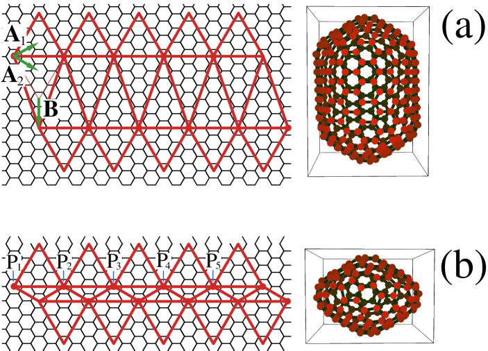
Figure 1: Geometric construction of the ”armchair” shapes of interest. The shape is cut out from the graphene plane and folded in an elongated (shape in panel (a)) or contracted (shape in panel (b)) or regular (not shown) icosahedron. Note that the points P₁, …, P₅ (panel (b)) are situated in polygon vertices of a (large) pentagon once the shape is folded.

The procedure is to cut out the outlined shape from the graphene plane and fold it into a polyhedron. The shapes that shall be considered can be loosely termed as elongated, regular or contracted icosahedra. Note that the construction results in twelve pentagonal carbon rings situated in vertices of (contracted or elongated) icosahedron. The equilibrated, minimal energy shapes obtained from the pieces of cut-out graphene plane are also displayed in Fig. 1. The numerical procedure that was used to obtain these shapes will be discussed in detail in Sec. 3. At this point, not only how the elongated shapes resemble carbon nanotubes, while the highly contracted shapes look almost like two cones glued together at their bases - there are two pentagonal carbon rings at the ”poles” of the shape (upper and lower points in shape depicted in panel (b) of Fig. 1), and the remaining ten pentagonal carbon rings are arranged around an ”equator” of the shape, in the polygon vertices of two parallel large pentagons rotated with respect to each other by an angle of $\pi/5$ (the vertices of one of those pentagons are denoted by points P₁,…,P₅ in Fig. 1). The shapes can be uniquely characterized by the lengths of two vectors, ${\bf A}_{1}$ and ${\bf B}$, since $|{\bf A}_{1}|=|{\bf A}_{2}|$ (see Fig. 1). The lengths are integer multiples of the distance between the centers of neighbouring carbon hexagonal rings, i.e.

$$|{\bf A}_{1}| = |{\bf A}_{2}|=md,$$

$$|{\bf B}| = nd,$$

$$d = a\sqrt{3}$$ (1)

where $a$ is the nearest neighbor C-C distance in graphite. I shall adopt the convention that negative values of $n$ correspond to contracted shapes, so that the shapes in Fig. 1 can be described by $(m=2,n=2)$ (elongated icosahedron) and $(m=2,n=-2)$ (contracted icosahedron). The (regular) icosahedral fullerenes are obtained for $n=0$. The condition that has to be fulfilled by $m$ and $n$ integers is $n\geq-m$. For $n\gg m$, the construction results in capped armchair $(5m,5m)$ single-wall carbon nanotubes and that is the reason for giving the attribute ”armchair” to the chosen subset of shapes. The total number of carbon atoms ($N$) in the constructed shapes is

$$N=60m^{2}+20mn.$$ (2)

Similar geometrical construction can be used to generate to ”zig-zag” or chiral (helical) shapes [18]. However, as the main intention of this work is in application of a continuum elasticity theory, the precise structure and atomic symmetry of the shape is of no importance, and only its shape matters in this respect. It should be noted here that the construction results in single-shell or single-wall carbon shapes/molecules. All the effects that are specific to multishell structures, in particular van der Waals interaction between the different shells are not treated in this work. For the application of the continuum elasticity theory in presence of van der Waals interactions and/or surrounding elastic medium see e.g. Refs. [19, 20].

3 Finding the minimum-energy shapes

The mathematically constructed folded polyhedra will not represent the minimum energy shapes. Carbon atoms in a minimum-energy structure should be relaxed so that the nearest-neighbour C-C distances are close to their optimum value energywise. To account for these effects, one should have a reliable description of the energetics of carbon bonding. In this work, the C-C interactions are modeled using a relatively recent second-generation reactive empirical bond order potential by Brenner et al [22]. In this model, the potential energy ($E_{b}$) of a carbon structure is given by

$$E_{b}=\sum_{i}\sum_{j}\left[V^{R}(r_{ij})-b_{ij}V^{A}(r_{ij})\right],$$ (3)

where $r_{ij}$ is the distance between nearest-neighbour atoms $i$ and $j$, $V^{R}$ and $V^{A}$ are pair-additive repulsive and attractive attractions, respectively, and $b_{ij}$ is the bond order between the atoms $i$ and $j$ that approximately accounts for the anisotropy of C-C bonding and for the many-body character of C-C interactions by including effectively the three-body contributions to $E_{b}$. The detailed description of the potential, together with all relevant parameters can be found in Ref. [22]. Similar potential models have been successfully employed in previous research of carbon structures (see e.g. Refs. [16, 17]).

The geometrically constructed, folded shape is used as the initial guess of the structure. The local minimum of $E_{b}$ in the configurational space spanned by coordinates of all carbon atoms is found using the conjugate gradient technique described in Ref. [21]. The conjugate gradient technique optimizes all the coordinates at once, proceeding through a sequence of steps along the ”noninterfering” or ”conjugate” direction in the configurational space, so that a minimization along a particular direction does not spoil the effect of minimization in other conjugate directions. Similar procedures have been used for the same purposes in Refs. [12, 13, 14].

4 Energies of shapes and considerations based on elasticity theory

4.1 Infinitely long carbon cylinders (non-capped carbon nanotubes)

Conceptually the simplest shape that can be constructed from the graphene plane is the open-ended (non-capped) carbon nanotube. It does not result from the construction described in Sec. 2, but shall be examined first to enable a simple insight in the application of elasticity theory to the shapes of interest. I shall consider infinitely long single-walled armchair carbon nanotubes. The energetics of such shapes can be studied by applying the (one-dimensional) periodic boundary conditions to the carbon-nanotube unit cell (ring or several rings of atoms), so that the effective number of independent coordinates that have to be optimized with respect to total energy of the nanotube is relatively small. Figure 2 displays the energy of infinite, armchair-type carbon cylinders as a function of the squared cylinder curvature given by $\kappa=1/\langle R_{cyl}\rangle$. The mean radius of the cylinder, $\langle R_{cyl}\rangle$ was calculated from the relaxed atomic coordinates as

$$\langle R_{cyl}\rangle=\frac{\sum_{i}\sqrt{x_{i}^{2}+y_{i}^{2}}}{N},$$ (4)

where $N$ is the total number of atoms in the unit cell, ${\bf r}_{i}=(x_{i},y_{i},z_{i})$ is the position vector of the $i$-th carbon atom, and the cylinder axis coincides with the $z$-axis. The cylinder radius calculated from Eq. (4) is always very close to the analytical prediction for tube radius, $R=a/\{2\sin[\pi/(3m)]\}$. For example, for $(10,10)$ carbon nanotubes, Eq. (4) and the numerically calculated values of ${\bf r}_{i}$ yield nanotube radius of 6.802 Å, while the analytical prediction is 6.794 Å. The agreement becomes slightly worse with the decrease in the nanotube radius. The energies displayed in Fig. 2 are in fact excess energies per unit area of the structure (denoted by $A_{c}$; $A_{c}=3a^{2}\sqrt{3}/4$) and were calculated as

$$\frac{\Delta E}{A_{c}}=(E_{cylinder}^{per\;atom}-E_{graphene}^{per\;atom})\frac{4}{3a^{2}\sqrt{3}},$$ (5)

where $E_{cylinder}^{per\;atom}$ and $E_{graphene}^{per\;atom}$ are the energies per atom in the cylinder and in the graphene plane, respectively.

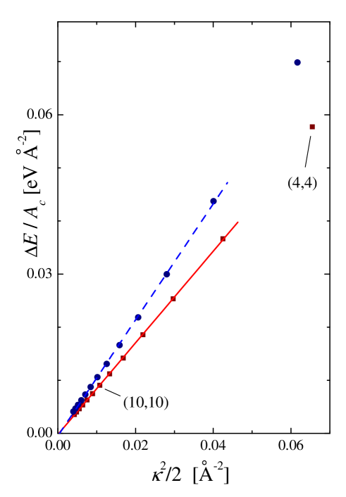
Figure 2: Excess energy per unit area as a function of squared cylinder (armchair carbon nanotube) curvature for the Tersoff potential [23] (circles) and the Brenner potential [22] (squares). The results for (4,4) and (10,10) armchair carbon nanotubes in this graph are denoted.

The calculations were carried out for two versions of the carbon-carbon potential which obviously predict different slopes of the dependence of the excess energy on squared curvature, but note that both curves are linear up to very large curvatures i.e. small radii of carbon nanotubes. Calculations with the early Tersoff potential [23] predict that somewhat larger energies are required to bend a piece of graphene plane in a cylinder with respect to those obtained by using the latest Brenner potential [22]. For the energy per unit atom in the graphene plane the two potentials predict $E_{graphene}^{per\;atom}=-7.39552$ eV (Tersoff’s potential) and $E_{graphene}^{per\;atom}=-7.39494$ eV (Brenner’s potential). More important difference between the two potentials is in the equilibrium C-C bond lengths they predict ($a=1.4605$ Å  and $a=1.4204$ Å  for the Tersoff and Brenner potential, respectively). The slopes of the lines shown in Fig. 2 ($c_{0}$) were obtained from fitting the calculated results pertaining to (5,5),(6,6),…,(16,16) carbon nanotubes, and for the Brenner and the Tersoff potential they are 0.863 $\pm$ 0.003 eV and 1.093 $\pm$ 0.006 eV, respectively (Tersoff obtained $c_{0}=1.02$ eV in Ref. [16]).

The demonstrated linear dependence of the excess energy per unit area on squared (mean) curvature can be easily understood from the examination of the geometry of bent network of graphene bonds. Consider a piece of graphene plane bent on a large cylinder of radius $R\gg a$. The most important change in the energetics of carbon network is due to a change in angles between the bonds, while the bond lengths remain the same as in graphene. Only the bond order term, $b_{ij}$ depends on the angles between bonds (see Eq. (3) and Refs. [22, 23]). By purely geometrical considerations it is easy to derive how the angles between the bonds change when the graphene plane is rolled onto a cylinder. If one assumes the plane to be inextensional, and considers large cylinder radii ($a/R\ll 1$) the change in energy per $i$-th atom is given by

$$\Delta E_{i}=\frac{1}{2}V^{A}(a)\left[\frac{\partial b_{ij}}{\partial\cos(\theta_{ijk})}\right]_{-1/2}\left(\frac{3a}{4R}\right)^{2},$$ (6)

which can also be written as

$$\frac{\Delta E}{A_{c}}=\frac{1}{2}V^{A}(a)\left[\frac{\partial b_{ij}}{\partial\theta_{ijk}}\right]_{2\pi/3}\frac{\kappa^{2}}{2},$$ (7)

where $j$ is the index of one of the three nearest neighbours of $i$-th atom, $k\neq j$ is any of the remaining two neighbors of $i$, and the angle between the $i-j$ and $i-k$ bonds is $\theta_{ijk}$ Explicitly written factor of 1/2 is a consequence of the fact that the energy in the Tersoff-Brenner potentials is situated in C-C bonds, and that each bond is shared by two atoms. Equation (7) is most easily derived by considering armchair or zig-zag carbon nanotubes, since in these cases one of the bonds is either parallel (zig-zag) or perpendicular (armchair) to the cylinder axis, but for $a/R\ll 1$, the relation holds also for helical nanotubes, i.e. for small curvatures the bending energies do not depend on the symmetry of the carbon nanotube. Note again that the analytical expression (7) accounts for the excess energy only in the limit of small curvatures $\kappa$ i.e. for radii of curvature that are large with respect to the graphene lattice constant.

Equation (7) shows that the excess energy per unit area is proportional to the squared curvature, in accordance with the results produced by calculations displayed in Fig. 2 (note, however, that only a curvature along one direction is accounted for by Eq. (7) which is sufficient for cylindrical surface). It furthermore predicts that the slope of this dependence is given by the properties of the interatomic potential (intriguingly, the factor of proportionality does not depend on the form of the repulsive part of potential for the class of bond order potentials given in Refs. [22, 23]). The slope $c_{0}$ can be easiliy read out from Eq. (7), and is calculated to be $c_{0}=0.8301$ eV and $c_{0}=1.0152$ eV for Brenner’s and Terssof’s potentials respectively. This is fairly close to the slopes obtained numerically. The small difference can be attributed to the fact that Eq. (7) is valid only for small curvatures, (or large radii, $a/R\ll 1$), i.e. it includes only the lowest order contribution of curvature (quadratic). For tubes of small radii, higher order terms are expected to be of importance. In fact, if one restricts the linear fit in Fig. 2 to smaller curvatures (from (12,12) to (16,16) nanotubes, $a/R<0.175$) one finds that the slopes are 0.839 eV and 1.036 eV, which is in significantly better agreement with the prediction of Eq. (7). Note that for (5,5) nanotubes, $a/R=0.414$, which means that the tubes of such small radii are already in the region where condition $a/R\ll 1$ does not hold, and the predictions of Eq. (7) are not expected to be very accurate.

The key conclusion of this subsection is that the excess energy per carbon atom ($\Delta E$) of an infinitely long carbon cylinder can be reliably estimated from

$$\frac{\Delta E}{A_{c}}=c_{0}\frac{\kappa^{2}}{2},$$ (8)

where $c_{0}$ is the elastic constant of the graphene plane related to the energetics of its bending (the bending rigidity), which, for infinitensimal curvatures, can be calculated from the knowledge of the interatomic interactions in graphene as in Eq. (7). This equation holds irrespectively of the details of the interatomic interactions, which only change the value of $c_{0}$ but not the functional dependence displayed in Eq. (8), which was illustrated by the examination of energetics predicted by two different models of C-C interactions [22, 23]. Equation (8) can also be understood without reference to atomic structure of the carbon nanotube by interpreting its left hand side as the bending energy per unit area of the material.

4.2 Icosahedral fullerenes

Icosahedral fullerenes are ($m,n=0$) subset of shapes considered in Sec. 2. They are more complex than the infinite carbon nanotubes from the standpoint of elasticity theory since they contain twelve pentagonal disclinations situated at vertices of an icosahedron. The excess energy of icosahedral fullerene relative to a piece of infinite graphene sheet with the same number of atoms is thus a result of both bending (and possibly stretching) of the sheet and the energy required to create disclinations. In order to calculate the bending contribution to the energy, one should have some information on the geometry of the minimal energy shape of the icosahedral fullerene. The pentagonal disclination can be constructed in a graphene plane, starting from the center of a hexagon, and cutting the plane in two directions that make an angle of 60 degrees - these cuts can be easily seen in the geometrical constructions in Fig. 1. The smaller, cut-out piece of graphene is discarded and the remaining (larger) piece of graphene is then folded to rejoin the edges of the cut. The shape of minimal energy that the remaining piece of graphene adopts is a cone, since it costs less energy to bend the C-C bonds than to stretch them (it is convenient to imagine a circular piece of graphene plane with a hexagon in its center). The shape will in fact be a truncated cone (or a conical frustum), since the pentagonal ring at the top of the cone will be flat and parallel to the larger base of the cone. The precise description of the shape depends on the values of two-dimensional Young’s modulus and bending rigidity. For materials like graphene (whose stretching requires much more energy than bending), the conical frustum is an excellent approximation of the minimal-energy shape. From purely geometrical considerations, the half angle of the cone is easily shown to be $\sin^{-1}(5/6)$. Shapes of crystalline, hexagonally coordinated membranes with pentagonal disclinations have been studied in Ref. [14], and many of the features discussed there apply also to the case of graphene. The icosahedral fullerene is a bit more complicated from a single cone since it contains twelve pentagonal carbon rings. It seems plausible that the fullerene shape should be well described by union of twelve truncated cones. The radius of the larger base of a particular cone is restricted by the presence of other cones. To illustrate these geometrical considerations, in Fig. 3 the shape of $(m=4,n=0)$ icosahedral fullerene is displayed (left column of images), which is in a minimum of total energy, obtained numerically as discussed in Sec. 3. The images in the right column of Fig. 3 display a union of twelve cones with half angles of $\sin^{-1}(5/6)$ whose larger bases just touch. Note that this geometrical construction is an excellent approximation to the calculated minimal energy shape. Its small drawback is that its total area (without inclusion of the areas of the larger bases of the cones) is smaller from the total area of the fullerene shape which is manifested is Fig. 3 by the appearance of ”holes”. Note also that the regions where these holes appear are almost flat in the numerically calculated minimal energy shape of the fullerene, and their contribution to the bending energy should thus be small.

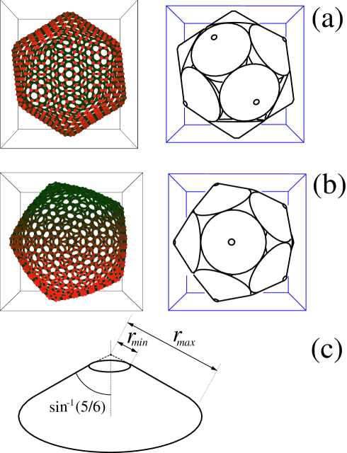
Figure 3: Panel (a): Equilibrated, minimal energy $(m=4,n=0)$ shape (left) and its approximation by twelve conical frusta whose smaller bases centers are situated at the vertices of an icosahedron (right). Panel (b): Same as in panel (a), only viewed from a different point. Panel (c): Elementary building block of the shapes shown in right columns of panels (a) and (b) - conical frustum whose half-angle is $\sin^{-1}(5/6)$. The quantities relevant to Eq. (11) are denoted.

Having such a good representation of the shape, it is possible to directly proceed to the calculation of its bending energy. In the continuum elastic theory of membranes [24], the bending energy ($H_{b}$) is represented as

$$H_{b}=\frac{1}{2}\int_{\rm{Surface}}dS\left(c_{0}\kappa^{2}+2c_{G}\gamma\right),$$ (9)

where $c_{0}$ is the bending rigidity discussed in the previous subsection, $c_{G}$ is the Gaussian rigidity, $dS$ is the infinitensimal element of the shape surface, and $\kappa$ and $\gamma$ are the mean and Gaussian curvature of the surface, respectively (if $R_{1}$ and $R_{2}$ are the principal radii of curvature, $\kappa=R_{1}^{-1}+R_{2}^{-1}$, and $\gamma=(R_{1}R_{2})^{-1}$). Note that for a cylindrical surface, $\gamma=0$ and $\kappa=1/R_{cyl}$ ($R_{1}=R_{cyl}$, $R_{2}=\infty$) in every point of the surface, and the total bending energy integrates to $H_{b}/A=c_{0}\kappa^{2}/2$, where $A$ is the total area of the cylinder (without the bases). This is in agreement with Eq. (8). For conical surfaces, the gaussian curvatures are also zero everywhere, so the total bending energy of the approximated fullerene shape will depend only on $c_{0}$. Integrating Eq. (9) over the surface of a cone whose half-angle is $\beta$, one finds that the bending energy of a cone ($H_{b}^{c}$) is

$$H_{b}^{c}=\frac{\cos^{2}\beta}{\sin\beta}\pi c_{0}\ln\left(r_{max}/r_{min}\right),$$ (10)

which for the cones with $\beta=\sin^{-1}(5/6)$ yields [16]

$$H_{b}^{c}=\frac{11\pi}{30}c_{0}\ln\left(r_{max}/r_{min}\right),$$ (11)

where the meaning of $r_{min}$ and $r_{max}$ is illustrated in panel (c) of Fig. 3 - these are the distances of the upper and lower bases of the conical frustum from the cone apex measured along the cone face. The value of $r_{min}$ can be easily evaluated due to the fact that the smaller base of the frustum is a pentagon of carbon atoms. There is some ambiguity, however, since the pentagon is to be approximated by a circle. If the circumradius of the pentagon is identified with the radius of the smaller base of the cone, one obtains that $r_{min}=3a\sqrt{50+10\sqrt{5}}/25\approx 1.021a$, which is the upper bound for $r_{min}$. The identification of the radius of the smaller base of the cone with the inradius of the pentagon yields $r_{min}=3a\sqrt{25+10\sqrt{5}}/25\approx 0.826a$, which is the lower bound for $r_{min}$. In any case, $r_{min}=fa$, where $f$ is a numerical factor between 0.826 and 1.021. The value of $r_{max}$ is half of the shortest distance between the two apices of the neighboring cones measured along the cone faces. From Figs. 1 and 3, one finds that $r_{max}=3(m-2)a/2+r_{min}$, and by using Eq. (2) one obtains that

$$\frac{r_{max}}{r_{min}}=\frac{3}{2f}\sqrt{\frac{N}{60}}+\frac{f-1}{f}.$$ (12)

It is obviously quite convenient to choose $f=1$, closer to the upper bound for $r_{min}$, so that the total excess energy of the icosahedral fullerene can be written as

$$\Delta E(N)=12\left[\lambda_{5}+\frac{11\pi}{60}c_{0}\ln\left(\frac{N}{60}\right)+\frac{11\pi}{30}c_{0}\ln\left(\frac{3}{2}\right)\right]+E_{holes}.$$ (13)

The multiplicative factor of 12 in the above equation is due to sum of the energies of twelve cones that make the shape surface, and $\lambda_{5}$ is the core energy of the pentagonal disclination which contains the local effects associated with the atomic structure of carbon pentagon and its immediate neighborhood. The contribution of the part of the fullerene surface that was not covered by the union of cones to the total energy was denoted by $E_{holes}$. Note that this quantity should represent a quite small correction to the total energy (see Fig. 3) and is not expected to depend strongly on $N$, since the area of the ”holes ” is proportional to $N$, while their mean curvature is approximately proportional to $1/\sqrt{N}$ (inverse radius of the fullerene, see Eq. (9)). Although one could easily invent a nice geometrical model to estimate this contribution, it is possible to proceed further by noting that Eq. (13) can also be written as

$$\Delta E(N)=\Delta E(C_{60})+\left[\frac{11\pi}{5}c_{0}\ln\left(\frac{N}{60}\right)\right],$$ (14)

where $\Delta E(C_{60})$ is the total excess energy of C₆₀ for which the calculation with the Brenner potential predicts $\Delta E(C_{60})=26.744$ eV. Figure 4 displays the results of numerical minimization of total energy of icosahedral fullerenes together with the prediction of Eq. (14) with $c_{0}=0.863$ eV taken from the analysis of infinite carbon cylinders. It seems more sensible to choose this value of $c_{0}$ rather than the one predicted by Eq. (7) which is appropriate for small curvatures, since close to the smaller bases of the truncated cones, condition $a/R\ll 1$, where $R$ is the radius of curvature is not fulfilled. Thus, a usage of a somewhat larger value of $c_{0}$ obtained from the numerical analysis of infinite carbon cylinder should approximately account for the contribution of terms like $(a/R)^{p}$, $p>2$ to the bending energy of the shapes studied. Note, however, that the (infinitensimal) analytical value of $c_{0}$ (0.83 eV) and the one obtained from the study of infinite carbon cylinders (0.863 eV) are quite similar, and one could also chose to work with the analytical value of $c_{0}$ with comparable success (see below).

Figure 4: Numerically calculated excess energies of icosahedral fullerenes (squares) and the prediction of Eq.(14) (line).

It can be seen in Fig. 4 that the agreement between the calculated values and those predicted by Eq. (14) is excellent (note that there are no fit parameters). Very small deviations can be mostly attributed to the fact that the regions around the larger bases of the cone are constrained by the continuity of the fullerene surface, and deviation from the cone shape is thus expected. It is to a certain extent surprising that the predictions of Eq. (14) are so precise, especially concerning the fact that the excess energy of C₆₀ figures in it as a parameter. Buckminsterfullerene is certainly not expected to be reliably described by the elasticity theory, since there are no atoms on the cone faces, only C-C bonds. Yet, the elasticity theory results maintain their meaning down to fullerenes of very small sizes and small number of atoms. By examining the energies of individual atoms in the icosahedral fullerenes it is possible to proceed a bit further and to estimate the value of the core energy, $\lambda_{5}$. For example, in $(m=4,n=0)$ fullerene shown in Fig. 3, the energies of atoms in pentagonal rings are -6.959 eV, while atoms situated in hexagonal carbon rings have energies of about -7.38 eV, depending on their position (see Eq. (3)). The energies of atoms in pentagonal rings do not change significantly with increasing the size of the fullerene, which is a consequence of the local nature of this energy. All this suggests that $\lambda_{5}=5[-6.9587-(-7.3949)]$ eV $=2.18$ eV, where -7.3949 eV is the energy per atom in the infinite graphene plane, predicted by the Brenner potential. Equation (14) does not depend (formally) on this quantity, but it can be calculated from Eq. (13) which yields $\lambda_{5}^{elast}=1.83$ eV ($E_{holes}$ was set to zero), in a quite nice agreement with the number obtained from the detailed atomic description of the icosahedral fullerenes, especially in a view of all the details involved in the approximation of the fullerene shape. This also confirms that $E_{holes}$ is indeed negligible part of the total energy.

4.3 Capped carbon nanotubes, elongated icosahedral fullerenes

Using the same reasoning outlined in the previous subsection, it is easy to construct an approximate shape of the elongated icosahedral fullerene ($n\neq 0$). These can be approximated by the union of twelve conical frusta and a cylinder whose length is $na\sqrt{3}$, and radius $15ma/(2\pi)$ (a finite-length piece of armchair (5$m$, 5$m$) carbon nanotube). The excess elastic energy can be thus written as

$$\Delta E(m,n)=12\left[\lambda_{5}+\frac{11\pi c_{0}}{30}\ln\left(\frac{3m}{2}\right)\right]+\frac{2\pi^{2}c_{0}}{5\sqrt{3}}\frac{n}{m}+E_{holes},$$ (15)

which could also be parameterized by the total number of atoms, $N$, and $n$. The first term in the expression for energy in Eq. (15) is the sum of the local and bending energies associated with the twelve equal pentagonal disclinations (conical frusta), and the second one corresponds to the bending energy of the finite length cylinder. The third term is again the energy associated with the ”holes” in the geometrical construction, as discussed in the previous subsection. Note that for $n=0$, Eq. (15) reduces to Eq. (13). Although the geometrical construction yielding Eq. (15) is quite simple, it has a small drawback in that the areas of the cones and of the cylinder in between them overlap to a small extent. Angles between the surfaces of the cones and the cylinder at the points in which the entities nearly touch are small but nonvanishing, which is another drawback of the proposed construction. More elaborate constructions are possible, but are not needed (Fig. 6).

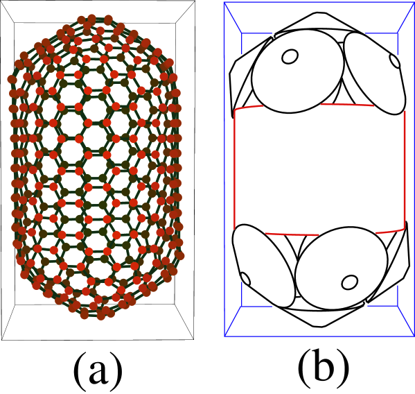
Figure 5: Panel (a): Numerically calculated equilibrium shape of $(m=2,n=4)$ elongated icosahedral fullerene. Panel (b): Approximation of shape using geometrical construction leading to Eq. (15).

Equation 15 can be approximated by

$$\Delta E(m,n)=\Delta E(C_{60})+\left[\frac{22\pi}{5}c_{0}\ln\left(m\right)+\frac{2\pi^{2}c_{0}}{5\sqrt{3}}\frac{n}{m}\right],$$ (16)

which simply states that the excess energy of the shape is equal to the sum of the excess energy of the icosahedral fullerene and the bending energy of the cylinder inserted in between its two ”halves” (see Fig. 5). This equation is, however, an approximation, since it is based on the assumption that the excess energies associated with the holes in the geometrical constructions are the same for the icosahedral fullerene and the elongated icosahedral fullerene, which is not exactly the case (compare Figs. 5 and 3). It furthermore contains an assumption that the elastic energies of holes do not depend on $m$ and $n$ integers characterizing the structure. Nevertheless, an excellent account of the numerical data is obtained which can be seen from Fig. 6. Note again that the analytical results presented in Fig. 6 represent the predictions of the elasticity theory without fit parameters.

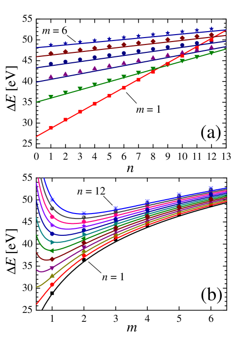
Figure 6: Panel (a): Excess energies of elongated icosahedral fullerenes (capped carbon nanotubes) as a function of elongation number ($n$) with $m$ as a parameter of the curves. Full symbols correspond to numerically calculated excess energies, while lines correspond to the predictions of elasticity theory in Eq. (16). Panel (b): Same data as in panel (a) with the roles of $m$ and $n$ numbers interchanged.

4.4 Contracted icosahedral fullerenes

The contracted icosahedral fullerenes are more complicated from the shapes considered thus far. Construction of their geometrical approximation is not simple mostly due to specific geometrical constraints that the ten pentagonal disclinations situated around the equator of the shape are subjected to. When $n$ vanishes, the area around each of the disclinations is well represented by a cone with an angle of $2\sin^{-1}(5/6)$ which was clearly demonstrated in subsection 4.2. When $n$ decreases (i.e. increases in absolute value), the two large pentagons parallel to the shape equator whose vertices coincide with five pentagonal disclinations (see Fig. 1) approach each other. This constrains the shape of the area around these pentagonal disclinations. As the cone was such an useful approximation of the area around pentagonal disclinations for shapes studied in subsections 4.2 and 4.3, it seems reasonable to try to describe the contracted icosahedral fullerenes also as union of cones, ten (those arranged around the equator of the shape) of which belong to one category, and two (the ones at the two poles of the shape) to another. The two cones at the poles are easily constructed as in subsections 4.2 and 4.3 - these have the angles of $2\sin^{-1}(5/6)$. The area around ten remaining disclinations is dominated by two opposing geometrical constraints. As $n$ decreases, the angle subtended by a line that connects a particular disclination (point A in panel (b) of Fig. 7) and the one at the closest pole (point B) and a line that connects the disclination with the midpoint of a line drawn between the two nearest disclinations in the neigbouring pentagonal ring of disclinations (point C) also decreases - this angle is denoted with $\alpha_{1}$ in panel (b) of Fig. 7. On the other hand, the angles that are subtended by the lines $\overline{\rm{DA}}$ and $\overline{\rm{AE}}$ or $\overline{\rm{FA}}$ and $\overline{\rm{AG}}$ (see Fig. 7) increase when $n$ decreases. It is thus clear that the area around the disclination cannot be represented by a single cone. Nevertheless, it seems reasonable to approximate this area by a union of pieces of surfaces of two cones, each of them satisfying one of the two opposing geometrical constraints.

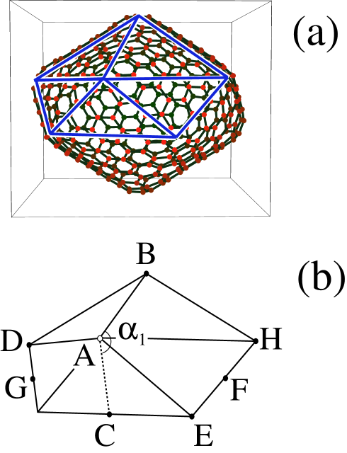
Figure 7: Panel (a): Equilibrium shape of ($m=3$, $n=-2$) contracted icosahedral fullerene. The characteristic pyramid-like shape is denoted by full lines. Panel (b): The pyramid-like shape with denotations discussed in the text.

The angle of one of the cones is about $\alpha_{1}$, which is given by

$$\alpha_{1}(n)=\cos^{-1}\left[\frac{1}{2\sin(\pi/5)}\right]+\cos^{-1}\left[\frac{\sqrt{3}m\tan(\pi/10)}{3m-2n}\right].$$ (17)

The angle of the second cone ($\alpha_{2}$) that is searched for is larger than $\alpha_{1}$, and the contribution of this half-cone to the total elastic energy of the area surrounding the disclination is thus smaller (see Eq. (10)). Nevertheless, the second cone is important since it contains a part of the total area surrounding the disclination, thus reducing the area available to the cone with angle $\alpha_{1}$. When $n=0$, both $\alpha_{1}$ and $\alpha_{2}$ angles should be $2\sin^{-1}(5/6)$. Note that when $n$ decreases, angle $\alpha_{2}$ changes in a significantly smaller range than $\alpha_{1}$, since it is importantly constrained by the fixed angle between lines $\overline{\rm{DA}}$ and $\overline{\rm{AH}}$ (see Fig. 7). Thus, I shall neglect the change of $\alpha_{2}$ with $n$ and set it to a constant

$$\alpha_{2} = 4\sin^{-1}(5/6)-\alpha_{1}(n=0)$$ (18)

$$= 4\sin^{-1}(5/6)-\cos^{-1}\left[\frac{1}{\sin(\pi/5)}\right]-\cos^{-1}\left[\tan(\pi/10)\right]$$

$$\approx 2.04\sin^{-1}(5/6),$$

which is obviously quite close to $2\sin^{-1}(5/6)$, as it should be, and which was chosen so that $\alpha_{2}+\alpha_{1}(n=0)=4\sin^{-1}(5/6)$, since I am further going to assume that each of the two cones takes exactly a half of the total area available to the disclination. Together with the choice for $\alpha_{2}$ in Eq. (18), this assumption shall yield the elastic disclination energy in the limit when $n=0$ equal to that characteristic of icosahedral fullerenes studied in subsection 4.2. Note that the axes of the two cones do not need to be identical - the two pieces of the conical surfaces can be rotated with respect to each other at will. It is also irrelevant how the particular cone (half)surface is constructed as long as the pieces of it are bounded by the arcs of the two bases subtending the same angle from the cone axis and the two lines (along the cone face) that connect the arc ends in the upper and lower base. Thus, there is a significant freedom in constructing a shape around the disclination, but for all of the thus constructed shapes the buckling energies are equal. Note also that for $n\neq 0$ points D, B, H, and E do not lie in a plane. The proposed construction is admittedly rather approximate. For example, one could object that the fractions of the total area belonging to each of the two cones should also (at least slightly) change with $n$. Nevertheless, the construction accounts for most important geometrical constraints imposed on the area around pentagonal disclinations situated around the equator of the shape due to the presence of neighboring disclinations. The exact answers to all of the objections regarding the proposed construction that could be easily put forth would require a solution of the nonlinear problem in the theory of elasticity, which is not the aim of this study - the aim is to obtain a simple insight in the energetics of the shapes using the simplest possible application of the elasticity theory, and to obtain, preferably analytic, expressions for the excess energies of such shapes.

Following the reasoning presented in the previous paragraph and using Eq. (10) for the calculation of bending energy of a cone with arbitrary half-angle, the total excess energy of the proposed geometrical approximation to the contracted icosahedral shapes is

$$\Delta E(m,n)=12\lambda_{5}+2E_{pole}(m,n)+10E_{equator}(m,n)+E_{holes},$$ (19)

where

$$E_{pole}=\frac{11c_{0}\pi}{30}\ln(3m-q),$$ (20)

$$E_{equator}=\frac{c_{0}\pi}{2}\ln(q)\left\{\frac{\cos^{2}[\alpha_{1}(n)/2]}{\sin[\alpha_{1}(n)/2]}+\frac{\cos^{2}(\alpha_{2}/2)}{\sin(\alpha_{2}/2)}\right\},$$ (21)

and

$$q=\frac{\sqrt{9m^{2}+3(3m-2n)^{2}}}{4}.$$ (22)

The last parameter ($q$) is simply a half of the distance (in units of $a$) between the two nearest neighboring disclinations situated at different pentagonal rings of disclinations around the equator of the shape (points A and E in Fig. 7).

Numerically calculated excess energies of the shapes and the predictions of Eq. (19) are shown in Fig. 8 and denoted by symbols and lines, respectively . In evaluating Eq. (19), $E_{holes}$ was set to zero, $\lambda_{5}=1.83$ eV was taken from the analysis of icosahedral fullerenes in subsection 4.2, and $c_{0}=0.863$ eV, as in the two previous subsections. Note again that there are no fitting parameters involved.

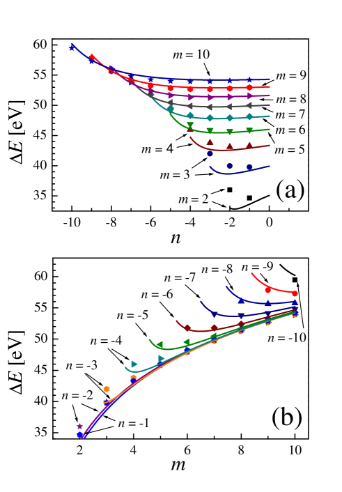
Figure 8: Panel (a): Excess energies of contracted icosahedral fullerenes as a function of $n$ with $m$ as a parameter of the curves. Full symbols correspond to numerically calculated excess energies, while lines correspond to the predictions of Eq. (19). Panel (b): Same data as in panel (a) with the roles of $m$ and $n$ numbers interchanged.

The agreement of the predictions of the elasticity theory with the numerical results is striking. In spite of all the approximations involved in the geometrical construction of the equilibrium shape, Eq. (19) both qualitatively and quantitatively accounts for the numerical data. The largest disagreement is found for the smallest shapes ($m=2$), but the curves correctly account for the appearance of minimum in excess energies for some finite $n$ (panel (a) of Fig. 8), and for the increase in excess energies when $|n|$ becomes comparable to $m$. It is worth noting that although the number of atoms in $n=-m$ structures is smaller than in $(m,n=0)$ structures (regular icosahedral fullerenes) by 20 $mn$ (see Eq. (2)), the total excess energies are still significantly larger in such structures, which is a consequence of an energetically unfavorable geometrical positions occupied by the ten disclinations around the equator of the shape. This consideration can also explain the minimum in excess energies obtained for some $n$ when $m$ is fixed - as the elongation number $n$ decreases, the number of atoms in the structure decrease, but the contribution to excess energy due to ten disclinations around the equator increase. The combined consequences of these two effects lead to the appearance of a minimum in excess energy as a function of $n$. Of the three types of shapes studied, the contracted icosahedral fullerenes typically have the largest excess energies per atom. For example, the excess energy of ($m=10$, $n=-10$) contracted fullerene ($\Delta E=59.47$ eV) that contains 4000 atoms is significantly larger from the excess energy of ($m=9$, $n=0$) regular icosahedral fullerene ($\Delta E=53.16$ eV) that contains larger number of atoms ($N=4860$).

5 Summary and conclusion

It has been shown that the insight in the geometry of the equilibrium shapes can be extremely useful in estimating their (excess) energies. Such an approach does not require detailed description of the interatomic interactions characteristic of a shape or molecule in question, instead it relies exclusively on the knowledge of elastic parameters of the material that the shape (shell) is made of. In the studies presented in this article, the parameters that were necessary for reliable estimation of energy were the local energy of pentagonal ring of carbon atoms ($\lambda_{5}$), and the bending rigidity of graphene plane ($c_{0}$). Both of these parameters derive from the quantum-mechanical nature of bonding of atoms (see Eq. (7)) that make the shape. Surprisingly enough, it has been demonstrated that the application of the simplest theory of elasticity yields reliable results even for shapes made of a small number of atoms, i.e. in the regime where its applicability is not to be expected. For all of the shapes considered, the knowledge of the two-dimensional Young’s modulus of graphene [24] was not needed, which suggests that in such shapes almost all of the elastic energy is of the bending type, while the energies associated with stretching are negligible . For shapes in which the geometrical constraints on the shape are strong (as in the case of contracted icosahedral fullerenes), the application of elasticity theory may be involved and complicated. Nevertheless, the identification of the constraints and their effects on the allowed shapes yields an additional insight in the energetics of the shapes and its behaviour within a certain class of shapes studied.

References

- [1] Kroto H W, Heath J R, O’Brien S C, Curl R F and Smalley R E 1995 Nature (London) 318 162
- [2] Ijima S 1991 Nature 354 56
- [3] Ge M and Sattler K 1994 Chem. Phys. Lett. 220 192
- [4] Krishnan A, Dujardin E, Treacy M M J, Hugdahl J, Lynum S and Ebbesen T W 1997 Nature 388 451
- [5] Smith B W, Monthioux M and Luzzi D E 1998 Nature 396 323
- [6] Han J, Globus A, Jaffe R and Deardorff G 1997 Nanotechnology 8 95
- [7] Hamada N 1993 Mater. Sci. Eng. B 19 181
- [8] Coluci V R, Galvao D S and Jorio A 2006 Nanotechnology 17 617
- [9] Vanderbilt D and Tersoff J 1992 Phys. Rev. Lett. 68 511
- [10] Fraenkel-Conrat H and Singer B 1999 Phil. Trans. R. Soc. Lond. B 354 583
- [11] Kroto H W and McKay K 1988 Nature 331 328
- [12] Lidmar J, Mirny L and Nelson DR 2003 Phys. Rev. E 68 051910
- [13] Nguyen T T, Bruinsma R F and Gelbart W M 2005 Phys. Rev. E 72 051923
- [14] Seung H S and Nelson D R 1988 Phys. Rev. A 38 1005
- [15] Baker T S, Olson N H and Fuller S D 1999 Microbiol. Mol. Biol. Rev. 63 862
- [16] Tersoff J 1992 Phys. Rev. B 46 15546
- [17] Robertson D H, Brenner D W and Mintmire J W 1992 Phys. Rev. B 45 12592
- [18] Terrones M, Terrones G and Terrones H 2002 Struct. Chem. 13 373
- [19] Ru C Q 2001 J. Mech. Phys. Solids 49 1265
- [20] He X Q, Kitipornchai S, Wang C M and Liew K M 2005 International Journal of Solids and Structures 42 6032
- [21] Hager W W and Zhang H 2005 Siam J. Optim. 16 170
- [22] Brenner D W, Shenderova O A, Harrison J A, Stuart S J, Ni B and Sinnott S B 2002 J. Phys.: Condens. Matter 14 783
- [23] Tersoff J 1989 Phys. Rev. B 39 5566
- [24] Landau L D and Lifshitz E M 2002 Theory of Elasticity (Oxford: Butterworth-Heinemann)
- [25] Lobkovsky A F 1996 Phys. Rev. E 53 3750
- [26] Witten T A and Li H 1993 Europhys. Lett. 23 51